Abstract
This study accounted for and analyzed the carbon emissions of 13 cities in Jiangsu Province from 1999 to 2021. We compared the simulation effects of four models—STIRPAT, random forest, extreme gradient boosting, and support vector regression—on carbon emissions and performed model optimization. The random forest model demonstrated the best simulation performance. Using this model, we predicted the carbon emission paths for the 13 cities in Jiangsu Province under various scenarios from 2022 to 2040. The results show that Xuzhou has already achieved its peak carbon target. Under the high-speed development scenario, half of the cities can achieve their peak carbon target, while the remaining cities face significant challenges in reaching their peak carbon target. To further understand the factors influencing carbon emissions, we used the machine learning interpretation method SHAP and the features importance ranking method. Our analysis indicates that electricity consumption, population size, and energy intensity have a greater influence on overall carbon emissions, with electricity consumption being the most influential variable, although the importance of the factors varies considerably across different regions. Results suggest the need to tailor carbon reduction measures to the differences between cities and develop more accurate forecasting models.
1. Introduction
Since the industrial revolution, the global economy has developed rapidly, emitting large amounts of greenhouse gases, such as carbon dioxide, into the environment, resulting in global warming and a series of environmental problems [1,2,3]. The global average temperature increase of 0.85 °C from 1880 to 2012 had risen to more than 1 °C by 2018. According to the IPCC, global environmental problems will be further exacerbated if the increase exceeds 1.5 °C [4,5]. With economic development, China’s energy consumption has increased dramatically. To actively reduce global greenhouse gas emissions, the government of China has set the goal of “China strives to achieve carbon peak by 2030, and carbon neutrality by 2060” [6,7,8].
Data accounting is fundamental for realizing carbon neutrality and carbon peak targets [9]. The current accounting methods for carbon emissions include the input–output method, life cycle assessment method, and emission factor method [10,11,12]. The input–output and life cycle assessment methods are complex and difficult to calculate [13]. The emission factor method estimates carbon emissions by multiplying energy activity data by emission factors; the data can usually be obtained from reliable sources such as yearbooks, making the emission factor method the mainstream approach [14]. Carbon emission rights have become an important discourse right for countries to compete. Therefore, it is crucial to conduct regional carbon emission accounting [15].
Models are effective tools for predicting the timing of carbon peaking and neutrality, exploring the factors influencing carbon emissions, and analyzing strategies for emission reduction [16]. Numerous models are available for carbon emission research, including the STIRPAT model [17], LMDI factor decomposition model [18], and environmental Kuznets curve [19]. Traditional statistical models often treat the relationship between carbon emissions and their influencing factors as a simple linear relationship of the same proportion, which makes it difficult to explain the complex nonlinear relationship, leading to poor fitting results in regression analysis [20,21,22,23]. With the rapid development of big data and computer science, machine learning has increasingly been used to solve complex scientific problems [24]. Machine learning, as a branch of artificial intelligence, employs certain algorithms to guide computers to use the input data, constantly learn the laws between the data, and optimize the calculation to arrive at a reasonable model [25]. In regional carbon emission research, machine-learning-based statistical models, such as BP neural networks [26] and support vector machines [27], have been successfully applied. Traditional methods generally rely more on human-set feature rules and perform poorly when facing complex and non-linear problems, whereas machine learning can process data sets and extract features through powerful generalization capabilities. It is critical to select the most suitable model by comparing multiple models to enhance the accuracy and reliability of carbon emission predictions [28,29,30]. The SHAP explanation method, derived from the shapely value in game theory, can deliver in-depth insights into model predictions by illustrating the contribution of each feature to specific predictions [31]. The combination of machine learning modeling and SHAP can further offer insights into the effect of characteristic variables on carbon emissions while predicting carbon emissions, and it can make machine learning easier to use through the current development of data sharing and intelligence [32].
Cities, as central hubs in politics, economics, and culture, are significant sources of energy use and CO2 emissions. Studies on regional emissions have employed the GIOWA model to analyze China’s emissions from 1980 to 2020 and develop reduction strategies [33]. Multiple linear regression was used to study emissions in the Yangtze River Delta for green development [34]. The STIRPAT model was improved with Adaboost to predict the carbon peak in Shandong [21], while the PSO-ELM model was applied to study decoupling and forecast emissions in Chongqing [30]. Nevertheless, there is a paucity of research comparing the carbon peaking scenarios of different cities within the same province, as well as investigating the pivotal factors affecting carbon peaking. Therefore, it is necessary to conduct peak carbon prediction on cities below to propose more comprehensive and precise planning.
As an economic powerhouse in eastern China and an important contributor to energy consumption and carbon emissions, Jiangsu Province is of practical significance to take the lead in the country in achieving peak GHG emissions, both in terms of intrinsic motivation and the need for external impacts [35]. This study aimed to achieve the following objectives: (1) Account for the carbon emissions of the cities in Jiangsu Province using statistical data from 1999 to 2021, adhering to the IPCC guidelines. (2) Construct machine learning models to analyze the carbon emissions of cities and identify the key factors influencing carbon emissions. (3) Predict the possible carbon emissions paths for each city in Jiangsu Province under three different scenarios.
2. Study Area and Methodology
2.1. Study Area and Data Sources
Jiangsu Province is located in the center of the Yangtze River Delta, covering an area of 107,200 square kilometers [36]. As shown in Figure S1, the province is divided into 13 prefecture-level cities. Jiangsu boasts a well-developed manufacturing industry with over 30 industrial sectors, contributing 13.3% to the national GDP, and ranks third in the country for carbon emissions [37]. Its development has been at the forefront of the country, and this high economic growth has been accompanied by increasing energy consumption and carbon emissions [38].
Relevant data for this study were obtained from multiple reliable publications and databases, including the 1999–2021 Statistical Yearbook of Jiangsu Province, statistical yearbooks of each city, China Emission Accounts and CEADs data sets (www.ceads.net.cn), the China Urban Greenhouse Gas Working Group, the National Economic Development Bulletin, and official government documents available on the websites of each city’s ecological and environmental bureaus, as well as through inquiries made via mayors’ mailboxes.
2.2. Methods of Accounting for Carbon Emissions
According to the IPCC Guidelines for National Greenhouse Gas Emission Inventories 2019 and based on the information from the Jiangsu Provincial Statistical Yearbook, this study comprehensively considered the energy consumption across five components: primary, secondary, and tertiary industries; residential life; and electric power consumption. The direct carbon emission from primary energy consumption refers to the carbon emission caused by fossil energy consumption [39]. The indirect carbon emission from secondary energy consumption is characterized by the electric power consumption of the entire society [40,41]. The specific carbon emission accounting formulas are provided in Equation (S1).
2.3. Model Building
In this study, traditional statistical models and machine learning models, including the STIRPAT model, extreme gradient augmentation (XGB), support vector regression (SVR), and random forest (RF) were selected to predict carbon emissions in the cities of Jiangsu Province. Figure 1 illustrates the working principles of the machine learning models. The traditional STIRPAT model originated from the IPAT equation. However, the IPAT equation can only change one factor at a time, presenting a major limitation. Therefore, the STIRPAT model was established, which can introduce multiple independent variables to analyze environmental factors [17].
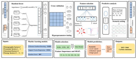
Figure 1.
Diagram showing how machine learning works.
Extreme gradient boosting (XGBoost) [42] is an efficient machine learning algorithm based on the gradient boosting tree algorithm, which trains models through decision trees. SVR [43] is typically used for data fitting. It uses a nonlinear transformation of the kernel function to highly dimensionalize the space and reduce the prediction error by hyperplane division. The RF [44] algorithm is based on Bagging integrated learning and decision trees. Each decision tree is trained by self-help and random repetitive sampling of data.
Jiangxi in the related study uses data from 2000 to 2020 for projecting carbon emissions from 2025 to 2035 [45]. The study in the Yangtze River Delta region uses carbon emission and socio-economic data from 2005 to 2019 for projecting [46]. Therefore, it is feasible for this study to use 75% of the statistical data from 1999 to 2021 for each city in Jiangsu Province as a training set and the remaining 25% as a test set for modeling. The variables in the prediction model are listed in Table S1. The output variable is carbon emissions (C), and the input variables are population size (P), GDP per capita (A), urbanization rate (U), industrial structure (IS), energy structure (ES), energy intensity (EI), and electricity consumption (EC). The performance of the model was assessed using R2, and the mean absolute error (MAE) and root mean square error (RMSE) were used to describe the magnitude of error between the predicted and true values.
2.4. Scenario Setting
In this study, 2021 was used as the base year to predict the trend of carbon dioxide emissions in the cities of Jiangsu Province from 2022 to 2040. Three scenarios were established: low-speed, medium-speed, and high-speed development. Based on the “14th Five-Year Plan”, the scenarios are divided into three stages of development: the first stage, 2022–2025; the second stage, 2026–2030; and the third stage, 2036–2040 [47]. The medium-speed development scenario is based on the development characteristics of the cities in Jiangsu Province, following the emission reduction policies, energy conservation measures, industrial restructuring, and other initiatives proposed in the “14th Five-Year Plan”. The influence factors were set based on the “Outline of the Fourteenth Five-Year Plan for the Development of the National Economy and Society and the Visionary Targets for the Year 2035” and the “Statistical Yearbook” of each city. The value of the change rate of each influencing factor is set, taking into account both historical inertia and the influence of relevant plans on each factor [48,49,50].
Under the low-speed scenario, population, GDP per capita, urbanization, and electricity consumption grow slowly. The tertiary industry’s share grows slowly, energy structure transformation is sluggish, and energy intensity decreases gradually. In the medium-speed scenario, these factors grow moderately, aligned with the next five-year plan and 2035 targets for each city, aiming for normal development carbon emission levels. Under high-speed development, population, GDP per capita, urbanization, and electricity consumption increase rapidly. The tertiary industry’s share and energy intensity decrease faster. The specific development model settings are listed in Table S2, and the scenario variables for each city in Jiangsu Province are listed in Tables S3–S15.
3. Results
3.1. Comparison of Carbon Emission Accounting Methods and Distributional Characteristics
The accounting method (IPCC method) used in this study was compared with the CEADs method [51] of the Tsinghua University Carbon Accounting Database and the PSO-BP method [52] for remote sensing inversion. The results are shown in Figure 2. The CEADs database is produced by Tsinghua University and other institutions using the IPCC and NDRC methods. The PSO-BP method utilizes remotely sensed light data and follows a “top-down” approach to estimate carbon emissions at the county scale in China. The final carbon emissions are obtained by deducting the carbon sequestration values of the terrestrial ecosystems.
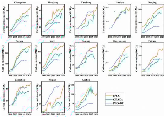
Figure 2.
Comparison of total carbon emissions obtained from different accounting methods.
The carbon emission trends obtained from the IPCC and CEADs methods are the same, but the curve of the IPCC method is slightly higher than that of CEADs. This difference may be because CEADs primarily account for energy and process aspects [51], while the IPCC accounts for carbon emissions from residents’ consumption (electricity consumption). The PSO-BP method shows a significant difference in data from the other two accounting methods, reporting much lower carbon emissions in Changzhou, Zhenjiang, Nanjing, Suzhou, and Xuzhou than the other two methods. The carbon emission trends in Yancheng, Huai’an, Nantong, and Yangzhou are similar across all three methods. The large difference between the PSO-BP and the other two data sets is likely because it uses nighttime light data from two different satellites and includes carbon sequestration values by terrestrial plants, which further increases data instability [52]. In general, the CEADs accounting method only publishes the emission factors of raw coal, oil, and natural gas, and it only accounts for cement processing in terms of process, which has certain limitations in the consideration of energy sources and processes. PSO-BP has a large error due to the limitations of its remote sensing data. In contrast, the accounting method provided by the IPCC takes into account the comprehensive consumption of nine energy sources and the social consumption of the residents, which is more suitable for the study of urban carbon emissions.
The changes in total carbon emissions from 1999 to 2021 in the cities of Jiangsu Province are shown in Figure 2. It indicates an overall increasing trend in carbon emissions across the 13 cities from 1999 to 2021 and a decrease in the growth rate in some cities in recent years. The carbon emissions trends accounted for in this study are consistent with the overall carbon emissions of Guangxi, Changsha, Chengdu, and Chongqing, which also show a significant upward trend [53,54,55]. In the cities of Huai’an, Taizhou, Yangzhou, and Xuzhou, the carbon emissions have been decreasing annually since 2015. The fluctuations in carbon emissions in the remaining cities have stabilized. Overall, most cities in Jiangsu Province have shown a fluctuating downward or stable trend in carbon emissions in recent years. These cities have a greater potential to reach their peak than cities whose carbon emissions are still on an upward trend.
The spatial distributions of carbon emissions in the cities of Jiangsu Province are shown in Figure 3 and Figure S2, in which the total annual average carbon emissions, carbon intensity, energy intensity, and per-capita carbon emissions of each city from 1999 to 2021 are categorized into three classes. Figure 3a shows that Suzhou and Nanjing fall within the highest average annual carbon emissions category, followed by Xuzhou and Wuxi. The remaining cities belong to the third category. Figure 3b–d show that Nanjing, Zhenjiang, Wuxi, and Suzhou rank first in per capita carbon emissions. In contrast, Nanjing and Xuzhou rank first in carbon emission intensity and energy intensity. A box–line diagram of the carbon emissions of each city in Jiangsu Province from 1999 to 2021 is shown in Figure S2. Suzhou has the highest annual carbon per capita emission (173 MtCO2), followed by Nanjing (150 MtCO2), while Suqian has the lowest (12 MtCO2), making Suzhou and Nanjing’s emissions approximately 14 and 12 times higher than that of Suqian, respectively. The carbon emissions in Jiangsu Province exhibit significant spatial variations, similar to the patterns observed in Guangdong Province (high in the north and low in the south) and Chongqing Municipality (high in the northeast of the main city) [56,57]. In conclusion, the spatial distribution of carbon emissions in Jiangsu Province, except for Xuzhou, was characterized by a decreasing trend from the south to the north.
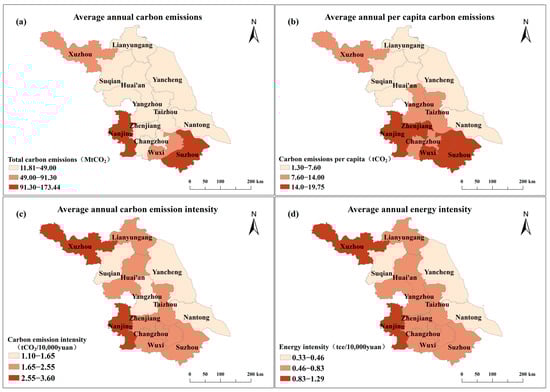
Figure 3.
Jiangsu Province: (a) total annual average carbon emissions, (b) per capita carbon emissions, (c) carbon intensity, and (d) energy intensity.
3.2. Comparison of Predictive Models
In this study, the STIRPAT model and XGB, SVR, and RF, which are three commonly used machine learning models with the advantages of accurate prediction in small samples, were selected to predict the carbon emissions of 13 cities and the whole province. The prediction results are presented in Tables S16 and S17. When modeling cities individually, the traditional STIRPAT model achieved an MAE and RMSE of less than 10 for most cities. However, four cities were poorly simulated, especially Zhenjiang, with R2 values lower than 0.8, with variations among cities. When the XGB model, a machine learning approach, was used to model cities individually, the simulation performance of the five cities was unsatisfactory, with R2 values on the test set lower than 0.8. Suzhou and Zhenjiang exhibited higher simulation error values, with Zhenjiang’s R2 on the test set at 0.614, indicating poor model performance. When the SVR model was used to model cities individually, three cities showed poor simulation performance, especially Huai’an and Suzhou. The R2 value of Suzhou was lower than 0.6, and the simulation error value of Suzhou was the highest among the three models, indicating relatively poor simulation performance. The RF model achieved MAE and RMSE values of less than 10 for most cities except for Suzhou, with R2 values greater than 0.876. Suzhou showed large simulation error values and poor performance, whereas other regions showed better simulation effects. Suzhou, Zhenjiang, and Huai’an had poor modeling performance, probably because the changes of the population, GDP per capita, and urbanization rate are relatively slow, and the urbanization rate especially showed a flat or even declining trend, which may have a certain impact on the model’s prediction. XGB and SVM models tend to overfit with limited data and many features, resulting in poor performance in data-scarce areas.
For the overall modeling of Jiangsu Province, the traditional STIRPAT model performed poorly, with an MAE and RMSE of more than 10 and an R2 of less than 0.9. Among the machine learning models, the XGB model had an MAE of more than 10, an RMSE of more than 20, and an R2 of 0.808, indicating high simulation error and poor performance. The SVR model showed an MAE and RMSE in the range of 10–14 and an R2 of 0.926, indicating some simulation errors. The RF model achieved MAE and RMSE values of less than 10 for both the training and test sets, with an R2 of 0.976 for the training set, indicating a strong simulation. In general, the performance of the machine learning model was better than that of the traditional STIRPAT model, the R2 values of the four models decreased as RF > SVM > STIRPAT > XGB, and the values of MAE and RMSE decreased as XGB > SVM > STIRPAT > RF. It is obvious that the RF model is optimal, with the highest value of R2 and the smallest error value among the four methods. The RF model is easy to implement; it avoids the problem of multiple covariances and overfitting of the model. Due to the random selection of sample data and attribute features, it has a strong anti-interference ability [58]. This is in line with the current performance of the machine learning model in carbon emission prediction, which often yields better results [59,60,61]. Therefore, the RF model was selected for the subsequent prediction analysis in this study.
3.3. Analysis of Influencing Factors
3.3.1. SHAP Analysis for Jiangsu Province
The prediction results of the RF model for the overall carbon emissions in Jiangsu Province can be explained using SHAP [62]. The left panel of Figure 4a shows the importance ranking plot of the characteristic variables, which represents the average SHAP value of all variables. The right panel shows the SHAP scatter summary plot of the characteristic variables. The SHAP values of variables on the left side of the X-axis play a negative role, while those on the right side play a positive role [63].
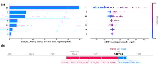
Figure 4.
(a) SHAP summary of carbon emissions based on random forest modeling. (b) SHAP-based localized explanatory maps.
As shown in the left panel of Figure 4a, the variable with the greatest impact on overall carbon emissions in Jiangsu Province was EC, followed by P and EI. Variables U and ES had smaller impacts, while IS and A did not show an obvious impact relationship based on the SHAP plot. In the right panel of Figure 4a, the samples of the EC, P, and EI variables on the left side are blue, and those on the right are red, which indicates that a higher social electricity consumption, larger population, and higher energy intensity are associated with higher carbon emissions. These associations mean that these three variables play a positive role in carbon emissions. The samples of the characteristic variable U are all red, indicating a positive effect on carbon emissions; the higher the urbanization rate, the higher the carbon emissions. For the variable ES, the left side of the plot is red, and the right side is blue, indicating that the energy structure and carbon emissions have a negative correlation; the energy structure with a high consumption has a negative effect on carbon emissions.
It is worth noting that the global aggregation is the average value of SHAP, and the local interpretation is the SHAP value calculated by the effect of individual characteristic variables on the model [64,65]. Figure 4b illustrates the local interpretation of the feature variables for the carbon emissions predicted by the RF model, with the base value being the average of the predictions, which was 802.10 MtCO2. In the figure, the red color refers to feature variables that have a positive effect on the base value, while the blue color indicates a negative effect, with the length of the arrows indicating the magnitude of the effect. For carbon emissions, EC was the most critical localized feature that positively affected carbon emissions. On the other hand, U and A negatively affected carbon emissions. When EC was 4.16 × 10⁸ MKW/h, P was 85.23 million, ES was 0.82, EI was 0.6, IS was 0.43, A was 6.51 × 10⁸ yuan, and U was 0.62; it pushed the model’s prediction to 1007.36 MtCO2, causing the model’s prediction to deviate from the baseline value and resulting in an increase in carbon emissions. In fact, the SHAP analysis of Jiangsu Province shows that EC, P, and EI drove the increase in carbon emissions in the global and local SHAP charts, because high electricity consumption generates more energy-consuming carbon emissions, and the increase in population and energy intensity also leads to further resource consumption and generates more energy consumption. Measures such as improving energy structure (ES), adjusting the proportion of fossil fuels such as coal, and using clean and renewable energy can reduce carbon emissions. Meanwhile, it will be beneficial to reduce carbon emissions to control the social use of electricity, implement energy-saving and emission-reduction measures, or use more solar and wind power generation.
3.3.2. Analysis of Characteristic Variables by Cities
In this study, the eigenvalue importance ranking of the RF model was used to analyze the factors influencing carbon emissions in the cities of Jiangsu Province. The eigenvalue output from the RF model were used to show the influence of the input variables on the model prediction results (Figure 5) [66]. The colors red, yellow, purple, blue, and green correspond to EC, EI, P, IS, and A, respectively, the variables with the greatest influence in modeling each city. The feature importance ranking shows that in 7 of the 13 cities in Jiangsu Province, EC is the variable that contributes the most to carbon emissions. For the remaining cities: in Huai’an and Zhenjiang, EI has the most significant impact; in Nanjing and Suqian, P is the most important contributing factor; in Yangzhou and Lianyungang, IS and A are the most important variables. The contribution of U is not prominent among the influencing factors. Most cities have two or more characteristic variables that affect the model outputs. The city-specific modeling results show that electricity consumption is the main factor affecting carbon emissions in Jiangsu Province. However, the electricity consumption contribution is insignificant in Huai’an, Suqian, and Lianyungang. Instead, Huai’an is primarily influenced by energy intensity and industrial structure, Suqian by population and GDP per capita, and Lianyungang by GDP per capita and urbanization rate. This indicates large differences in the influencing factors among different cities.
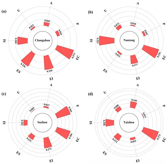
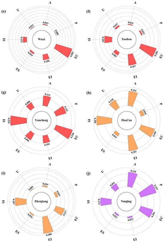
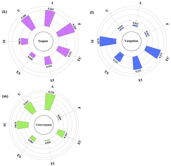
Figure 5.
Importance ranking map of features based on random forest modeling: (a) Chang zhou, (b) Nan tong, (c) Su zhou, (d) Tai zhou, (e) Wu xi, (f) Xu zhou, (g) Yancheng, (h) Huai’an, (i) Zhen jiang, (j) Nan jing, (k) Su qian, (l) Yang zhou, (m) Lian yun gang.
3.4. Scenario Analysis
In this study, a carbon emission prediction model constructed using random forest was combined with three scenario development modes to predict the carbon emission trends of cities in Jiangsu Province from 2022 to 2040. The time of the carbon peak was derived for each city, as shown in Figure 6.
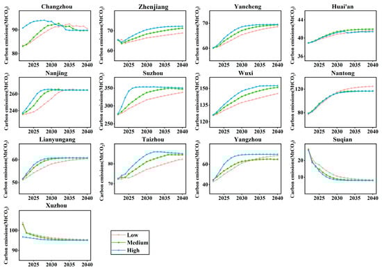
Figure 6.
Carbon emission simulation and forecasting results for district cities in Jiangsu Province for the period 2022–2040.
Based on the projections under different scenarios, all cities and municipalities in Jiangsu Province can achieve the target of peak carbon emissions by 2036. Notably, Xuzhou and Suqian have already reached their peak carbon; Changzhou, Nanjing, Lianyungang, Suzhou, and Yangzhou need to adopt a high-speed development mode to achieve peak carbon by 2030; and Huai’an, Nantong, Taizhou, Yancheng, Wuxi, and Zhenjiang are projected to reach peak carbon only by 2036.
Under the three scenarios, carbon emissions in Xuzhou and Suqian generally show a decreasing trend. According to the carbon emission accounting results (Figure 2), Xuzhou’s carbon emissions peaked in 2013, whereas Suqian’s peaked in 2022 and then declined steadily. Changzhou and Nanjing can reach peak in all three developmental modes from 2022 to 2040. In the high-speed development mode, Changzhou will reach its carbon peak in 2028, and Nanjing will realize the carbon peak in 2030; in the medium-speed development mode, both Changzhou and Nanjing will reach the carbon peak in 2032; in the low-speed development mode, Changzhou and Nanjing will realize the carbon peak in 2032 and 2036, respectively. Huai’an, Lianyungang, Nantong, Suzhou, Taizhou, Yancheng, and Yangzhou can achieve peak carbon emissions under the below development modes. Under the high-speed development mode, Lianyungang, Suzhou, and Yangzhou can achieve peak carbon emissions by 2030; Huai’an and Taizhou can achieve peak carbon emissions by 2032; and Nantong and Yancheng can achieve peak carbon emissions by 2034. Under the medium-speed development mode, these cities can achieve peak carbon emissions only after 2032. Wuxi and Zhenjiang can only reach peak carbon in the high-speed development mode and only reaching peak carbon in 2035 and 2036, respectively.
Overall, among the three development modes, the medium-speed mode aligns with national and urban plans for normal development up to 2040. It allows for routine allocation of socio-economic development and energy inputs. The low-speed mode slows socio-economic development and reduces energy and resource inputs, suitable for low government investment. The high-speed mode accelerates the rate of reaching peak carbon emissions but demands rapid population growth and urbanization, aggressive industrial and energy transitions, and intense economic development pressure on cities.
4. Discussion and Policy Suggestions
4.1. Model Advantage
Compared with traditional carbon emission studies that mostly focus on large-scale cities and provincial capitals, the degree of refinement is insufficient, and the traditional models used usually have limited prediction accuracy [67,68,69,70]. In this study, the prediction accuracy of carbon emission is improved by introducing a machine learning model, and the influencing factors are deeply explored by using SHAP analysis. This method visualizes the different impacts of each variable on urban carbon emissions, which helps to formulate more targeted carbon emission reduction programs and promote the cities to realize the peak of carbon emissions as soon as possible.
4.2. Policy Suggestions
To realize the peak carbon target in Jiangsu Province as soon as possible, it is necessary to choose a carbon reduction pathway according to local conditions and make comprehensive considerations based on the influencing factors of different cities, and a few policy points are provided in the context of this study. Cities that can achieve the 2030 peak carbon target under the high-speed development mode need to further optimize the industrial structure on the basis of maintaining the stable development of the ecological economy to achieve the peak carbon target in advance [71,72]. Cities with greater difficulty in reaching the peak in 2030 need to accelerate urbanization, enhance industrial transformation, promote green economic development, optimize the energy structure and intensity, and complete the goal of reaching the carbon emission peak [73,74,75]. Based on the contribution of different urban influencing factors, the comprehensive promotion of the realization of the goal of peak carbon will be based on the integration of economic factors and energy factors. In terms of emission reduction measures, they can promote the optimization of industrial structure and eliminate industries with backward production capacity as soon as possible; they can further strengthen scientific and technological research and development and promote the development of energy-saving and emission reduction technologies. In terms of energy, they can reduce the consumption of fossil energy, especially raw coal, and vigorously develop clean energy to reduce energy intensity. These measures can, to a certain extent, help Jiangsu Province realize the goal of carbon peaking [76,77,78].
5. Conclusions
In this study, the carbon emissions of 13 cities in Jiangsu Province were accounted for using the IPCC method, and the carbon emissions were predicted separately by the traditional and the machine learning models. The SHAP interpretation method of machine learning was used to analyze Jiangsu Province as a whole, and subregions were analyzed using the feature importance ranking method. Significant differences were found among different cities. The RF model with the best simulation performance was used to predict the carbon emissions of each city in Jiangsu Province under three scenarios from 2022 to 2040. Most cities are projected to reach the carbon peak in 2030, while the remaining cities are expected to reach the carbon peak in 2036. This study makes up for the shortcomings of regionalized differences in carbon peaking in city scale, which provides references for carbon peaking and policy making in other cities.
In addition, there are errors in carbon emission forecasts, mainly due to the small number of statistical indicators and different statistical calibers of each city. Only four models were selected for comparison and selection in modeling. In the future, with more carbon emission monitoring data of each city, the advancement of the intelligence level will allow more accurate models to be applied to the field of carbon emission prediction.
Supplementary Materials
The following supporting information can be downloaded at https://www.mdpi.com/article/10.3390/su162310450/s1, Equation S1: Carbon emission accounting formulas. Figure S1: Overview of the study area. Figure S2: Carbon Emission Box-Line Chart for Cities in Jiangsu Province. Table S1: Description of predictive model variables. Table S2: Carbon Emission Scenario Setting for Cities in Jiangsu Province. Table S3: Changzhou City Scenario Variable Settings (%). Table S4: Huai’an City Scenario Variable Settings (%). Table S5: Lianyungang City Scenario Variable Settings (%). Table S6: Nanjing City Scenario Variable Settings (%). Table S7: Nantong City Scenario Variable Settings (%). Table S8: 6 Suzhou City Scenario Variable Settings (%). Table S9: Suqian City Scenario Variable Settings (%). Table S10: Taizhou City Scenario Variable Settings (%). Table S11: Wuxi City Scenario Variable Settings (%). Table S12: Xuzhou City Scenario Variable Settings (%). Table S13: Yancheng City Scenario Variable Settings (%). Table S14: Yangzhou City Scenario Variable Settings (%). Table S15: Zhenjiang City Scenario Variable Settings (%). Table S16: STIRPAT model simulation performance. Table S17: Machine learning model simulation performance.
Author Contributions
W.Y.: writing—original draft, data collection. L.C.: data curation, formal analysis. T.K.: data curation. H.H.: conceptualization, fund acquisition. D.L.: methodology. K.L.: investigation. H.L.: writing—review and editing, supervision, fund acquisition. All authors have read and agreed to the published version of the manuscript.
Funding
This work was supported by the Special Science and Technology Innovation Program for Carbon Peak and Carbon Neutralization of Jiangsu Province (no. BE2022612) and the National Natural Science Foundation of China (no. 42077430).
Institutional Review Board Statement
Not applicable.
Informed Consent Statement
Not applicable.
Data Availability Statement
The original contributions presented in the study are included in the article/Supplementary Materials; further inquiries can be directed to the corresponding author.
Conflicts of Interest
The authors declare no competing interests.
References
- Zong, J.F.; Sun, L.; Bao, W. Situation analysis and development suggestion regarding carbon emission peaking. In Proceedings of the 4th International Workshop on Renewable Energy and Development (IWRED), Electr Network, Hangzhou, China, 24–26 April 2024; IOP: Bristol, UK, 2024. [Google Scholar]
- Kaygusuz, K. Energy and environmental issues relating to greenhouse gas emissions for sustainable development in Turkey. Renew. Sustain. Energy Rev. 2009, 13, 253–270. [Google Scholar] [CrossRef]
- Rahman, M.M.; Alam, K. CO2 Emissions in Asia-Pacific Region: Do Energy Use, Economic Growth, Financial Development, and International Trade Have Detrimental Effects? Sustainability 2022, 14, 5420. [Google Scholar] [CrossRef]
- Garland, M. Towards a Just and Sustainable Blue Economy: An Examination of the Blue Economy Narrative for Long Island Sound. Ph.D. Thesis, Southern Connecticut State University, New Haven, CT, USA, 2019. [Google Scholar]
- Lewis, S.C.; King, A.D.; Perkins-Kirkpatrick, S.E.; Mitchell, D.M. Regional hotspots of temperature extremes under 1.5 °C and 2 °C of global mean warming. Weather Clim. Extrem. 2019, 26, 100233. [Google Scholar] [CrossRef]
- Zhu, S. Present Situation of Greenhouse Gas Emission in Beijing and the Approach to Its Reduction. China Soft Sci. 2009, 9, 93–98. [Google Scholar]
- Wang, P.; Zhong, Y.Y.; Yao, Z.A. Modeling and Estimation of CO2 Emissions in China Based on Artificial Intelligence. Comput. Intell. Neurosci. 2022, 2022, 6822467. [Google Scholar] [CrossRef]
- Lai, Y.; Xia, X.; Li, F.; Peng, R. Current Situation, Challenges and New Trend of Carbon Emissions in Beijing: A Comparative Study on Climate Action in Six International Metropolises. Urban Stud. 2023, 30, 83–89. [Google Scholar]
- Li, H.; Cao, H.; Liu, L.; Xing, B.; Pan, X.; Wen, X.; Ge, W. Research Status and Technology Path of Low-carbon Manufacturing under the Background of Emission Peak and Carbon Neutrality. J. Mech. Eng. 2023, 59, 225–240. [Google Scholar]
- Long, Y.; Yoshida, Y.; Liu, Q.L.; Zhang, H.R.; Wang, S.Q.; Fang, K. Comparison of city-level carbon footprint evaluation by applying single- and multi-regional input-output tables. J. Environ. Manag. 2020, 260, 110108. [Google Scholar] [CrossRef]
- Wang, Y.; Liu, Y.; Cui, S.; Wang, Z. Research on Carbon Emission and Reduction Potential of Building Ceramics in China. Mater. Rev. 2018, 32, 3967–3972. [Google Scholar]
- Liu, T.; Wu, Z.; Chen, C.; Chen, H.; Zhou, H.Y. Carbon Emission Accounting during the Construction of Typical 500 kV Power Transmissions and Substations Using the Carbon Emission Factor Approach. Buildings 2024, 14, 145. [Google Scholar] [CrossRef]
- Geng, Y.; Dong, H.; Xi, F.; Liu, Z. A Review of the Research on Carbon Footprint Responding to Climate Change. China Popul. ·Resour. Environ. 2010, 20, 6–12. [Google Scholar]
- Kim, B.S.; Jang, W.S.; Lee, D.E. Analysis of the CO2 emission characteristics of earthwork equipment. Ksce J. Civ. Eng. 2015, 19, 1–9. [Google Scholar] [CrossRef]
- He, J.X.; Zhao, W.H. Research on The Path of Carbon Emission Trading in China Under The Double Carbon Background. Probl. Ekorozwoju 2023, 18, 81–88. [Google Scholar] [CrossRef]
- Xu, S.X.; Lv, Z.Y.; Wu, J.Z.; Chen, L.J.; Wu, J.H.; Gao, Y.; Lin, C.M.; Wang, Y.; Song, D.; Cui, J.C. Prediction method of regional carbon dioxide emissions in China under the target of peaking carbon dioxide emissions: A case study of Zhejiang. Meteorol. Appl. 2024, 31, 2203. [Google Scholar] [CrossRef]
- Zhang, X.W.; Cao, W.J. Research on Influence Factors of Carbon Emission Based on STIRPAT Model in Jilin Province. In Proceedings of the International Conference on Social Science, Public Health and Education (SSPHE), Guangzhou, China, 5–6 May 2017; pp. 37–42. [Google Scholar]
- Zheng, L.X. Carbon emission measurement method of heavy industry based on LMDI decomposition method. Int. J. Glob. Energy Issues 2023, 45, 113–124. [Google Scholar] [CrossRef]
- Chen, P.J. An Empirical Study of the Carbon Emission Kuznets Curve in Tianjin. In Proceedings of the 2nd International Conference on Air Pollution and Environmental Engineering (APEE), Xi’an, China, 15–16 December 2019; IOP: Bristol, UK, 2019. [Google Scholar]
- Dong, J.; Zong, M.; Chen, J. A method to predict the carbon emissions of civil aviation based on stirpat model. Environ. Eng. 2014, 32, 165–169. [Google Scholar]
- Kong, D.P.; Dai, Z.; Tang, J.Y.; Zhang, H. Forecasting urban carbon emissions using an Adaboost-STIRPAT model. Front. Environ. Sci. 2023, 11, 1284028. [Google Scholar] [CrossRef]
- Chen, Z.M.; Ohshita, S.; Lenzen, M.; Wiedmann, T.; Jiborn, M.; Chen, B.; Lester, L.; Guan, D.B.; Meng, J.; Xu, S.Y.; et al. Consumption-based greenhouse gas emissions accounting with capital stock change highlights dynamics of fast-developing countries. Nat. Commun. 2018, 9, 3581. [Google Scholar] [CrossRef]
- Luo, X.C.; Liu, C.K.; Zhao, H.H. Driving factors and emission reduction scenarios analysis of CO2 emissions in Guangdong-Hong Kong-Macao Greater Bay Area and surrounding cities based on LMDI and system dynamics. Sci. Total Environ. 2023, 870, 161966. [Google Scholar] [CrossRef]
- Guo, H.N.; Wu, S.B.; Tian, Y.J.; Zhang, J.; Liu, H.T. Application of machine learning methods for the prediction of organic solid waste treatment and recycling processes: A review. Bioresour. Technol. 2021, 319, 124114. [Google Scholar] [CrossRef]
- Aleskerov, F.; Demin, S.; Richman, M.B.; Shvydun, S.; Trafalis, T.B.; Yakuba, V. Constructing an Efficient Machine Learning Model for Tornado Prediction. Int. J. Inf. Technol. Decis. Mak. 2020, 19, 1177–1187. [Google Scholar] [CrossRef]
- Chen, Z.X.; Liu, L.K.; Li, C.H. Prediction and Control of Carbon Emissions of Electric Vehicles Based on BP Neural Network under Carbon Neutral Background. In Proceedings of the International Conference on Neural Networks, Information and Communication Engineering, Qingdao, China, 27–29 August 2021. [Google Scholar]
- Huo, Z.G.; Zha, X.T.; Lu, M.Y.; Ma, T.Q.; Lu, Z.C. Prediction of Carbon Emission of the Transportation Sector in Jiangsu Province-Regression Prediction Model Based on GA-SVM. Sustainability 2023, 15, 3631. [Google Scholar] [CrossRef]
- Zhao, Y.H.; Liu, R.R.; Liu, Z.S.; Liu, L.; Wang, J.J.; Liu, W.X. A Review of Macroscopic Carbon Emission Prediction Model Based on Machine Learning. Sustainability 2023, 15, 6876. [Google Scholar] [CrossRef]
- Kayakus, M. Forecasting carbon dioxide emissions in Turkey using machine learning methods. Int. J. Glob. Warm. 2022, 28, 199–210. [Google Scholar] [CrossRef]
- Liu, B.; Chang, H.D.; Li, Y.; Zhao, Y.P. Carbon emissions predicting and decoupling analysis based on the PSO-ELM combined prediction model: Evidence from Chongqing Municipality, China. Environ. Sci. Pollut. Res. 2023, 30, 78849–78864. [Google Scholar] [CrossRef]
- Utkin, L.; Konstantinov, A. Ensembles of Random SHAPs. Algorithms 2022, 15, 431. [Google Scholar] [CrossRef]
- Rashid, A.; Rasheed, R.; Ngah, A.H.; Amirah, N.A. Unleashing the power of cloud adoption and artificial intelligence in optimizing resilience and sustainable manufacturing supply chain in the USA. J. Manuf. Technol. Manag. 2024, 35, 1329–1353. [Google Scholar] [CrossRef]
- Wang, H.; Wei, Z.J.; Fang, T.; Xie, Q.J.; Li, R.; Fang, D.B. Carbon emissions prediction based on the GIOWA combination forecasting model: A case study of China. J. Clean. Prod. 2024, 445, 141340. [Google Scholar] [CrossRef]
- Wang, Y.; Wu, Y. Analysis and forecast of carbon emissions in the Yangtze River Delta region. J. Anhui Agric. Univ. 2023, 50, 1051–1058. [Google Scholar]
- Cheng, A.; Han, X.R.; Jiang, G.G. Decomposition and Scenario Analysis of Factors Influencing Carbon Emissions: A Case Study of Jiangsu Province, China. Sustainability 2023, 15, 6718. [Google Scholar] [CrossRef]
- Huang, M.L.; Jiang, H. The Spatial and Temporal Characteristics of Surface Ultraviolet Radiation and Total Ozone in Urban Agglomeration of Yangtze River Delta. In Proceedings of the Joint Workshop on Urban Remote Sensing, Shanghai, China, 20–22 May 2009; IEEE: Piscataway, NJ, USA, 2009; pp. 436–442. [Google Scholar]
- Lv, T.G.; Zhao, Q.; Zhang, X.M.; Hu, H.; Geng, C. Spatiotemporal pattern and influencing factors of regional carbon emission efficiency: An empirical analysis of Jiangsu Province in China. Int. J. Low-Carbon Technol. 2023, 18, 1048–1059. [Google Scholar] [CrossRef]
- He, J.; Yan, W.; Duan, X.; Zou, H. Location Identification and Spatial Evolution of Industrial Heat Sources Along Yangtze River in Jiangsu Province. Resour. Environ. Yangtze Basin 2022, 31, 995–1005. [Google Scholar]
- Li, Z.; Li, Y.B.; Shao, S.S. Analysis of Influencing Factors and Trend Forecast of Carbon Emission from Energy Consumption in China Based on Expanded STIRPAT Model. Energies 2019, 12, 3054. [Google Scholar] [CrossRef]
- He, Y.Y.; Wei, Z.X.; Liu, G.Q.; Zhou, P. Spatial network analysis of carbon emissions from the electricity sector in China. J. Clean. Prod. 2020, 262, 121193. [Google Scholar] [CrossRef]
- Lv, W. Calculation and Analysis of Greenhouse Gas Emission Factors for Organizational Purchased Electricity. Environ. Sci. Technol. 2014, 37, 199–204. [Google Scholar]
- Sun, Y.; Lü, L.; Cai, Y.K.; Lee, P. Prediction of black carbon in marine engines and correlation analysis of model characteristics based on multiple machine learning algorithms. Environ. Sci. Pollut. Res. 2022, 29, 78509–78525. [Google Scholar] [CrossRef]
- Gou, G.H. SVR-based prediction of carbon emissions from energy consumption in Henan Province. In Proceedings of the 3rd International Conference on Advances in Energy Resources and Environment Engineering (ICAESEE), Harbin, China, 8–10 December 2017; IOP: Bristol, UK, 2017. [Google Scholar]
- Chang, Z.Y.; Jiao, Y.M.; Wang, X.J. Influencing the Variable Selection and Prediction of Carbon Emissions in China. Sustainability 2023, 15, 13848. [Google Scholar] [CrossRef]
- Duo, L.; Zhong, Y.; Wang, J.; Chen, Y.; Guo, X. Spatio-temporal characteristics and scenario prediction of carbon emissions from land use in Jiangxi Province, China. Int. J. Environ. Sci. Technol. 2024. [Google Scholar] [CrossRef]
- Zou, X.; Sun, X.; Ge, T.; Xing, S. Carbon Emission Differences, Influence Mechanisms and Carbon Peak Projections in Yangtze River Delta Region. Resour. Environ. Yangtze Basin 2023, 32, 548–557. [Google Scholar]
- Yao, M.; Wang, M.; Lei, Y. Research on Shanghai Carbon Peak Forecast Based on STIRPAT Model. J. Fudan University. Nat. Sci. 2023, 62, 226–237. [Google Scholar]
- Liu, W.S.; Ren, D.C.; Ke, C.B.; Ying, W. Carbon Emission Influencing Factors and Scenario Prediction for Construction Industry in Beijing-Tianjin-Hebei. Adv. Civ. Eng. 2023, 2023, 2286573. [Google Scholar] [CrossRef]
- Liu, C.; Qian, X. Prediction of carbon emissions from energy consumption in China under the “dual carbon” goal. Resour. Sci. 2023, 45, 1931–1946. [Google Scholar] [CrossRef]
- Wang, S.J.; Mo, H.B.; Fang, C.L. Carbon emissions dynamic simulation and its peak of cities in the Pearl River Delta Urban Agglomeration. Chin. Sci. Bull. -Chin. 2022, 67, 670–684. [Google Scholar] [CrossRef]
- Liu, Z.; Guan, D.B.; Wei, W.; Davis, S.J.; Ciais, P.; Bai, J.; Peng, S.S.; Zhang, Q.; Hubacek, K.; Marland, G.; et al. Reduced carbon emission estimates from fossil fuel combustion and cement production in China. Nature 2015, 524, 14677. [Google Scholar] [CrossRef]
- Chen, J.; Gao, M.; Cheng, S.; Hou, W.; Song, M.; Liu, X.; Liu, Y.; Shan, Y. County-level CO2 emissions and sequestration in China during 1997-2017. Sci. Data 2020, 7, 391. [Google Scholar] [CrossRef]
- Gao, M.; Wu, X. Temporal and spatial characteristics and peak prediction of carbon emissions in Guangxi Zhuang Autonomous Region. Carsologica Sin. 2023, 42, 763–774. [Google Scholar]
- Liu, L.Y.; Tang, Y.L.; Chen, Y.Y.; Zhou, X.; Bedra, K.B. Urban Sprawl and Carbon Emissions Effects in City Areas Based on System Dynamics: A Case Study of Changsha City. Appl. Sci. 2022, 12, 3244. [Google Scholar] [CrossRef]
- Wei, Y.; Li, S.; Zhang, H. Temporal-spatial evolution of carbon emission and driving factors in the Chengdu-Chongqing urban agglomeration. China Environ. Sci. 2022, 42, 4807–4816. [Google Scholar]
- Wu, Z.; Wang, D.; Su, Y. Study on Spatial-temporal Variation and Influencing Factors of Urban Carbon Emissions in Guangdong Province Based on EDGAR Data. Areal Res. Dev. 2020, 39, 127. [Google Scholar]
- Xiang, S.-J.; Yang, C.-M.; Xie, Y.-Q.; Wang, D.; Wang, Z.-F.; Gao, M. Spatiotemporal Dynamic Evolution and Gravity Center Migration of Carbon Emissions in the Main Urban Area of Chongqing over the Past 20 Years. Huan Jing Ke Xue = Huanjing Kexue 2023, 44, 560–571. [Google Scholar] [CrossRef]
- Zhang, H.; Peng, J.Y.; Wang, R.; Zhang, M.X.; Gao, C.; Yu, Y. Use of random forest based on the effects of urban governance elements to forecast CO2 emissions in Chinese cities. Heliyon 2023, 9, e16693. [Google Scholar] [CrossRef] [PubMed]
- Zeng, H.; Sun, W.; He, W.; Guo, Y.; Guo, C. Study on the Carbon Emission Prediction Model for Railway Tunnel Construction Based on Machine Learning. Mod. Tunn. Technol. 2023, 60, 29–39. [Google Scholar]
- Singh, P.K.; Pandey, A.K.; Ahuja, S.; Kiran, R. Multiple forecasting approach: A prediction of CO2 emission from the paddy crop in India. Environ. Sci. Pollut. Res. 2022, 29, 25461–25472. [Google Scholar] [CrossRef] [PubMed]
- Sun, W.; Wang, Y.; Zhang, C. Forecasting CO2 emissions in Hebei, China, through moth-flame optimization based on the random forest and extreme learning machine. Environ. Sci. Pollut. Res. 2018, 25, 28985–28997. [Google Scholar] [CrossRef]
- Strumbelj, E.; Kononenko, I. Explaining prediction models and individual predictions with feature contributions. Knowl. Inf. Syst. 2014, 41, 647–665. [Google Scholar] [CrossRef]
- Lundberg, S.M.; Erion, G.; Chen, H.; DeGrave, A.; Prutkin, J.M.; Nair, B.; Katz, R.; Himmelfarb, J.; Bansal, N.; Lee, S.I. From local explanations to global understanding with explainable AI for trees. Nat. Mach. Intell. 2020, 2, 56–67. [Google Scholar] [CrossRef]
- Wang, S.; Ren, Y.; Xia, B. PM2.5 and O3 concentration estimation based on interpretable machine learning. Atmos. Pollut. Res. 2023, 14, 101866. [Google Scholar] [CrossRef]
- Park, J.; Lee, W.H.; Kim, K.T.; Park, C.Y.; Lee, S.; Heo, T.Y. Interpretation of ensemble learning to predict water quality using explainable artificial intelligence. Sci. Total Environ. 2022, 832, 155070. [Google Scholar] [CrossRef]
- Liu, K.; Zhang, Y.; He, H.; Xiao, H.; Wang, S.; Zhang, Y.; Li, H.; Qian, X. Time series prediction of the chemical components of PM2.5 based on a deep learning model. Chemosphere 2023, 342, 140153. [Google Scholar] [CrossRef]
- Wang, S.; Wang, Y.X.; Zhou, C.X.; Wang, X.L. Projections in Various Scenarios and the Impact of Economy, Population, and Technology for Regional Emission Peak and Carbon Neutrality in China. Int. J. Environ. Res. Public Health 2022, 19, 2126. [Google Scholar] [CrossRef]
- Huang, R.; Lu, Y.; Lu, M. Projection of Energy Consumption Carbon Emission Peak for Jiangsu, Zhejiang and Shanghai Under Different Energy Policies. Resour. Environ. Yangtze Basin 2017, 26, 15–25. [Google Scholar]
- Tang, J.; Zheng, J.; Yang, G.; Li, C.; Zhao, X. Carbon emission prediction in a region of Hainan Province based on improved STIRPAT model. Environ. Sci. Pollut. Res. Int. 2024, 31, 58795–58817. [Google Scholar] [CrossRef] [PubMed]
- Cao, L.; Li, M.; Zhang, L.; Cai, B. Research on Carbon Dioxide Emission Peaking in the Yangtze River Delta Urban Agglomeration. Environ. Eng. 2020, 38, 33. [Google Scholar]
- Li, S.; Ma, W.; Hao, H.; Zhao, J. CO2 emission characteristics and emission reduction measures of country energy consumption: A case study of Huailai County, Hebei Province. Chin. J. Environ. Eng. 2023, 17, 2277–2285. [Google Scholar]
- Zhao, M.; Lu, L.; Wang, S.; Bai, Z.; Zhang, N.; Luo, H.; Fu, J. Meta Regression Analysis of Pathway of Peak Carbon Emissions in China. Res. Environ. Sci. 2021, 34, 2056–2064. [Google Scholar]
- Song, P.; Zhang, H.; Mao, X. Research on Chongqing’s carbon emission reduction path towards the goal of carbon peak. China Environ. Sci. 2022, 42, 1446–1455. [Google Scholar]
- Ma, D.; Chen, W. China’s carbon emissions peak path-based on China TIMES model. J. Tsinghua Univ. Sci. Technol. 2017, 57, 1070–1075. [Google Scholar]
- Rashid, A.; Rasheed, R.; Altay, N. Greening manufacturing: The role of institutional pressure and collaboration in operational performance. J. Manuf. Technol. Manag. 2024; ahead of print. [Google Scholar] [CrossRef]
- Yan, G.; Zheng, Y.; Wang, X.; Li, B.; He, J.; Shao, Z.; Li, Y.; Wu, L.; Ding, Y.; Xu, W.; et al. Pathway for Carbon Dioxide Peaking in China Based on Sectoral Analysis. Res. Environ. Sci. 2022, 35, 309–319. [Google Scholar]
- Miao, A.-K.; Yuan, Y.; Wu, H.; Ma, X.; Shao, C.-Y. Pathway and Policy for China’s Provincial Carbon Emission Peak. Huan Jing Ke Xue = Huanjing Kexue 2023, 44, 4623–4636. [Google Scholar] [CrossRef]
- Zhao, Y.; Duan, X.Y.; Yu, M. Calculating carbon emissions and selecting carbon peak scheme for infrastructure construction in Liaoning Province, China. J. Clean. Prod. 2023, 420, 138396. [Google Scholar] [CrossRef]
Disclaimer/Publisher’s Note: The statements, opinions and data contained in all publications are solely those of the individual author(s) and contributor(s) and not of MDPI and/or the editor(s). MDPI and/or the editor(s) disclaim responsibility for any injury to people or property resulting from any ideas, methods, instructions or products referred to in the content. |
© 2024 by the authors. Licensee MDPI, Basel, Switzerland. This article is an open access article distributed under the terms and conditions of the Creative Commons Attribution (CC BY) license (https://creativecommons.org/licenses/by/4.0/).