An Urban Metro Section Flow Forecasting Method Combining Time Series Decomposition and a Generative Adversarial Network

Abstract

Urban metro cross-section flow is the passenger flow that travels through a metro section. Its volume is a critical parameter for planning operation diagrams and improving the service quality of urban subway systems. This makes it possible to better plan the drive for the sustainable development of a city. This paper proposes an improved model for predicting urban metro section flow, combining time series decomposition and a generative adversarial network. First, an urban metro section flow sequence is decomposed using EMD (Empirical Mode Decomposition) into several IMFs (Intrinsic Mode Functions) and a trend function. The sum of all the IMF components is treated as the periodic component, and the trend function is considered the trend component, which are fitted by Fourier series function and spline interpolation, respectively. By subtracting the sum of the periodic and trend components from the urban metro section flow sequence, the error is regarded as the residual component. Finally, a GAN (generative adversarial network) based on the fusion graph convolutional neural network is used to predict the new residual component, which considers the spatial correlation between different sites of urban metro sections. The Chengdu urban metro system data in China show that the proposed model, through incorporating EMD and a generative adversarial network, achieves a 15–20% improvement in prediction accuracy at the cost of a 10% increase in the calculation time, meaning it demonstrates good prediction accuracy and reliability.

1. Introduction

1.1. Forecast Methods

With the increasing scale of rail transit in developing countries, rail transit has officially entered the network operation stage. Accurate section flow prediction makes a reasonable rail vehicle traffic scheduling plan, selects the emergency rescue location, improves the passenger transportation efficiency, and reduces costs. It is also conducive to the sustainable development of cities [1]. Over decades, scholars have conducted in-depth research on the forecasting problem [2]. Short-term traffic forecasting models are mainly divided into three types: parametric models, non-parametric models, and hybrid models. Parametric models, including the ARIMA (Autoregressive Integrated Moving Average) model [3] and Kalman filtering [4], are usually based on statistical theory, and in the context of these models, it is a prerequisite that the time series data are stationary. Non-parametric models, such as k-proximity algorithms [5], artificial neural networks [6,7,8], SVMs (Support Vector Machines) [9], and language models [10], include a large number of families. Their main advantage is that they avoid setting some unnecessary parameters, thus avoiding noise impacts. Their main disadvantage is that the training model process is not transparent and requires a large amount of historical data and time. Hybrid models, on the other hand, can combine different models, overcoming the shortcomings of using a single model and making the resulting model more robust [11]. Among hybrid models [12,13], time series decomposition has become a very popular method in recent years. Time series decomposition extracts several relatively simple sub-sequences from raw data, and each component is fitted with the best suitable model, and the final accumulation is carried out to improve accuracy. Based on this approach, Huang et al. [14] invented the Hibert transform. In contrast to the wavelet and Fourier transforms, which have many limitations when processing complex signals, this transform can theoretically decompose any type of signal into a connotative-mode IMF [15], which can present a variety of frequencies, trends, and residual components. The earliest time series decomposition was applied to the short-term forecasting of temperature [16], finance [17,18], electricity loads [19], and hydrology [20,21], with good forecasting results being observed. However, combined time series decomposition models such as ARIMA and LSTM focus on a single series and rarely take into account the correlation of predicted samples. The advantages and disadvantages of the various models are shown in Table 1.

Table 1. Advantages and disadvantages of forecasting methods.

	Models	Advantages/Disadvantages
Parametric models	Linear regression	Advantages: The methods are easier to understand, and the results are easier to interpret. Disadvantages: Unable to predict complex sequences.
	ARIMA
	SARIMA
	…
Non-parametric models	SVM	Advantages: It can fit and predict most complex sequences. Disadvantages: The training process is opaque.
	KNN
	GCN
	LSTM
	BiLSTM
	…
Hybrid models	KNN-LSTM	Advantages: Combining the forecast results from multiple models gives a more accurate overall forecast. Disadvantages: Poor combination can predict performance degradation.
	LSTM-GCN
	EMD-SAE
	EMD-LSTM
	EMD-BiLSTM
	…

In order to solve the problem regarding the fact that sample correlation is not considered in time series decomposition, we decided to use a hybrid model that fuses EMD and GANs and is based on an STGCN (Space Time Graph Convolutional Network). We call the hybrid model STGCN-GAN, and through using EMD to separate the periodic part and the trend part of an original sequence and using GAN to predict the remaining unstable residual sequence due to the adversarial generation of GANs, it can predict complex sequences. First, this paper describes the extraction of passenger trip’s OD data from the subway automatic fare collection system and the calculation of the hourly passenger flow crossing each section according to the logit allocation method, carried out to obtain the time series of all the cross-sectional flows $X_i\left(t\right),(i=\mathrm{1,2},\dots ,N)$. Symbol $N$ is the number of sections between two adjacent stations in the urban metro system. Second, we decompose the original sequence $X_i\left(t\right)$ into several IMF components and a trend component, treating the sum of all IMF components as periodic components. Third, the periodic component refers to the cyclical fluctuation of the cross-sectional flows in a certain period of time. So, we used Fourier series for prediction. Fourth, the trend component represents the long-term characteristics of the railway-sectional passenger demand can be predicted by spline interpolation. It is assumed here that the seasonal and trend components are intrinsic for each railway section. Finally, the prediction error is regarded as the remaining components minus the seasonal and trend components from the original sequence $X_i\left(t\right)$. The residual part is much more difficult to predict than the seasonal and trend components due to its irregularities, and this has a great impact on passenger flows in adjacent down-sections. Therefore, it is more appropriate to use non-parametric methods to deal with the resident component individually in order to catch its long-term uncertainties. Due to the powerful ability of GAN learning complex distributions [22], we built a GAN model based on graph convolutional neural networks to predict the passenger volume of the railway sections. Figure 1 shows the framework for the prediction model proposed in this paper.

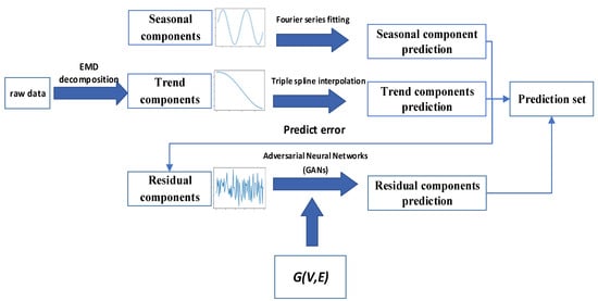
Figure 1. STGCN-GAN prediction model framework based on EMD.

The highlights of this article are summarized as follows:

(1)

An STGCN-GAN (Space Time Graph Convolutional Network–Generative Adversarial Network) hybrid prediction model based on EMD is proposed.

(2)

The model uses cross-sectional traffic data to make predictions, and the results show that the performance of the model is better than that of other baseline models such as those based on GCNs (Graph Convolutional Networks) and LSTM (Long Short-Term Memory), Bi-LSTM, STGCN, and STGCN-GAN. The prediction accuracy is generally improved at 15–50%.

(3)

The model achieved a 15–20% improvement in prediction accuracy at the cost of a 10% increase in the calculation time, meaning it demonstrates good prediction accuracy and reliability.

This article is divided into seven sections: The first section mainly discusses the advantages and disadvantages of various methods. Section 2 describes the details of the EMD time series decomposition method and seasonal, trend, and residual components. Section 3 focuses on datasets and data processing. Section 4 describes the use of Fourier series to predict seasonal components. Section 5 introduces the use of cubic spline interpolation to predict trend components. Section 6 presents the use of STGCN-GAN to predict the residual component. Section 7 presents the forecast results and formulates the train schedule based on the forecast results, and future directions for research and the conclusions that can be derived from the work described in this paper are also noted in this section.

1.2. Related Work

(a) Time series decomposition

EMD is a method used to decompose time series data into different components and then model and forecast these components independently [23]. Hamad et al. [15] were the first to use EMD to predict vehicle speeds on Fairfax highways to infer travel times. Chen et al. [24] directly treated time series as seasonal components and performed the Hibert transform, observing dynamic fluctuations in passenger flow through the time–frequency energy distribution revealed by Hilbert’s spectrum and achieving good predicting results. Yang et al. [9] used a time series forecasting hybrid model based on EMD and a SAE (Superimposed Auto Encoder), EMD-SAE, to predict traffic flow. They found that the SAE method, used to process all decomposed IMFs and residuals, may be able to solve the end effect problem. Huang [25] applied EMD to extract the intrinsic mode function of the traffic flow recorded by four adjacent sensors on a highway and intuitively presented the seasonal mode in the form of frequency through the Hilbert transform. The seasonal components can then be described as Fourier series based on the obtained frequencies, which improves the prediction accuracy of the seasonal components and predicts the remaining components by using a Bi-LSTM (Bi-directional Long Short-Term Memory) neural network.

(b) Generative adversarial networks

The GAN model was originally proposed by Goodfellow [26]. Originally, GANs were used for image recognition and generation. But more recently, GANs have been used to fit complex sequences. Alkilane [27] combined GANs and GCNs to predict short-term traffic flow. Several GCNs were constructed within a generator based on different perspectives such as similarity, correlation, and spatial distance, and remarkable results were obtained. Liang [28] proposed a SATP-GAN model based on self-attention and the generative adversarial network mechanism which showed improved prediction performance compared to a baseline model. Kun [29] proposed a generative adversarial model (GAN) with Long Short-Term Memory (LSTM) as the generator and deep multilayer perceptron (MLP) as the discriminator to predict a network traffic time series.

2. Methodology

2.1. Time Series Decomposition

Figure 1 shows the process through which the original cross-section flow time series can be decomposed into three component types: seasonal components, a trend component, and a residual component. Then, the seasonal components and trend component are fitted using the Fourier function and triple spline interpolation, respectively. The new residual component equals the original cross-section flow time series minus the addition of the Fourier function and triple spline interpolation, which is forecasted by the adversarial neural network; therefore, prediction results can be obtained from the Fourier function, triple spline interpolation, and the new residual component forecasted by the adversarial neural network.

Since the cross-sectional flow sequence $X_i\left(t\right)$ on urban metro sections has a seasonal, trendy character, the time series is decomposed into several IMF components, a trend component and residual component, via EMD. The process can be modelled as shown in Formula (1):

$$X_i\left(t\right)=P_i\left(t\right)+R_i\left(t\right)+V_i\left(t\right)$$

(1)

where $P_i\left(t\right)$ is the seasonal components, $R_i\left(t\right)$ is the trend component, and $V_i\left(t\right)$ is the residual component. The original sequence $X_i\left(t\right)$ and the residual component $V_i\left(t\right)$ are relevant to a certain urban metro section, so these functions are not only relevant to time but also space, while the seasonal component $P_i\left(t\right)$ and the trend component $R_i\left(t\right)$ are treated as functions of time only. For the sake of brevity, here, we ignore the space variant in the original sequence $X_i\left(t\right)$ and residual component $V_i\left(t\right)$ temperately.

EMD can handle non-linear and non-stationary data. The main idea behind EMD is to decompose the original time series of raw data into a limited number of oscillation modes based on its own local characteristic time scale. Each oscillation mode is similar to a harmonic function and is represented by an IMF. The IMFs must meet the following two conditions:

(a)

Throughout the data segment, the number of extremum points and the number of zero crossing points must be equal or have one difference.

(b)

At any moment, the average value of the upper envelope formed by the local maxima point and the lower envelope formed by the local maxima point is zero, that is, the upper and lower envelopes are locally symmetrical relative to the time axis.

First, all the extremum points in the sequence $X_i\left(t\right)$ are identified, and all the maximal and minimum points are fitted with cubic spline interpolation to form the upper and lower envelopes as $e_{i, max}\left(t\right)$ and $e_{i, min}\left(t\right)$, respectively. The average envelope $m_i\left(t\right)$ is as follows:

$$m_i\left(t\right)=\frac{1}{2}(e_{i, max}\left(t\right)+e_{i,min}\left(t\right))$$

(2)

In the second step, the intermediate signal $h_i\left(t\right)$ is obtained by subtracting the average envelope from the original sequence $X_i\left(t\right)$, which is the j^th IMF if both conditions (a) and (b) are met. If not, let $h_i\left(t\right)$ replace $X_i\left(t\right)$ for a second screening.

$$h_i\left(t\right)=X_i\left(t\right)-m_i\left(t\right)$$

(3)

$$h_i^{11}\left(t\right)=h_i\left(t\right)-m_i^{11}\left(t\right)$$

(4)

$$\dots$$

$$h_i^{1j}\left(t\right)=h_i^{1(j-1)}\left(t\right)-m_i^{1j}\left(t\right)$$

(5)

where $m_i^{11}\left(t\right)$ is the average envelope of $h\left(t\right)$. Repeat both steps (3) and (4) until $h_i^{1j}\left(t\right)$ satisfies conditions (a) and (b). Then, the j^th IMF will equal $h_i^{1j}\left(t\right)$.

$${IMF}_i^j\left(t\right)=h_i^{1j}\left(t\right)$$

(6)

The trend components $r_i^n\left(t\right)$, after the $j$^th IMF has been obtained, can be expressed as follows:

$$r_i^n(t)=X_i\left(t\right)-\sum _j{IMF}_i^j\left(t\right)$$

(7)

Revert $r_i^n\left(t\right)$ as the original signal and repeat Formulas (1)–(4) until the SD (Standard Deviation) is less than the threshold of 0.2.

$$SD={‖r_i^n\left(t\right)-r_i^{n-1}\left(t\right)‖}^2/{‖r_i^{n-1}\left(t\right)‖}^2$$

(8)

The original signal can be expressed as Formula (9):

$$X_i\left(t\right)=r_i^n(t)+\sum _j{IMF}_i^j\left(t\right)$$

(9)

In this way, we decompose the original sequence into n IMF modal functions and a trend. Now, perform a Hilbert transform on each IMF to find the instantaneous frequency of each IMF. The Hilbert transform is shown in Formula (10):

$$H\left({IMF}_i\left(t\right)\right)=\frac{1}{\pi }{\int }_{-\infty }^{+\infty }{(IMF}_i\left(t\right)/(t-\tau ))d\tau$$

(10)

The solution of the amplitude angle is shown in Formula (11):

$${\phi }_i\left(t\right)=\arctan \left(\frac{H\left({IMF}_i\left(t\right)\right)}{{IMF}_i\left(t\right)}\right)$$

(11)

The instantaneous frequency ${\omega }_i$ and cycle $T_i$ are shown in Formulas (12) and (13):

$${\omega }_i={d\phi }_i\left(t\right)/dt$$

(12)

$$T_i=1/{\omega }_i$$

(13)

The seasonalic component $P_i\left(t\right)$ can be reverted to Formula (14):

$$P_i\left(t\right)=a_0+\sum _{i=1}^n{a}_i\cos \left(2\pi {\omega }_{i}t\right)+b_i\sin \left(2\pi {\omega }_{i}t\right)$$

(14)

The trend component $R_i\left(t\right)$ is the cubic spline interpolation fitting of the trend component $r_i^n\left(t\right)$, represented by $L\left(r_i^n\right(t\left)\right)$, and the residual component is the original sequence needed to remove the seasonal component and the trend components due to the fact that the original sequence $X_i\left(t\right)$ is relevant to a certain urban metro section $i$; so, we add variant $i$ as $X_i\left(t\right)$ and the residual component as $V_i\left(t\right)$:

$$R_i\left(t\right)=L\left(r_i^n\right(t\left)\right)$$

(15)

$$V_i\left(t\right)=X_i\left(t\right)-P_i\left(t\right)-R_i\left(t\right)$$

(16)

2.2. GAN Methodology

The principle and structure of a generative adversarial network (GAN) is introduced in this section. The GAN model was originally proposed by Goodfellow [26] and usually consists of two parts: generator G and discriminator D. The GAN structure is shown in Figure 2. Generator G learns how to generate real data until the discriminator is indistinguishable from real data. The goal of the discriminator is to accurately identify whether the input sample is real or not from the generator. In this way, G and D constitute a dynamic “game process”.

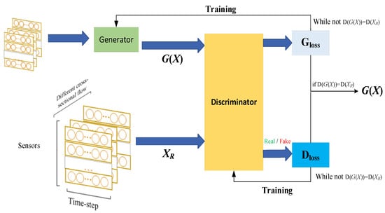
Figure 2. The architecture of the STGCN-GAN.

The purpose of G’s loss function in Equation (23) is to maximize the probability that $D$ will accept that the data generated by G are real.

$$G_{loss}=-\mathit{log}\left(1-D\left(G\left(X\right)\right)\right)$$

(17)

The training of the discriminator D is a binary classification, and the goal is to distinguish between the real data and the generated data; that is, the D output of the real data is close to 1. So, the discriminator uses cross-entropy as the loss function, as shown in Equation (24). $X_R$ represents the real dataset. $X$ is the forecasting dataset.

$$D_{loss}=-\mathit{log}\left(D\left(G\left(X\right)\right)\right)-\mathit{log}\left(1-D\left(X_R\right)\right)$$

(18)

During the training of the GAN model, the two neural networks D(·) and G(·) are alternately optimized. The generator continuously optimizes itself based on the gap between the generated sample and the real sample. As the number of iterations increases, the samples generated by the generator gradually more closely resemble the real sample. When the discriminator cannot distinguish whether the sample is real or not, the two networks reach equilibrium.

3. Data Processing

We considered Chengdu Metro card data as an example for our research. In this study, automatic card swiping data from the Chengdu Metro pertaining to a period ranging from 12 April to 5 May 2021 were collected. The Chengdu Metro dataset has sufficient temporal and spatial coverage to cover working days and weekends during holidays. The original data format is shown in Table 2.

Table 2. Partial raw data.

Transaction Date	Enter Time	Enter Station Name	Exit Time	Exit Station Name
23 April 2021	10:53:02	Chunxi Road	11:17:08	Tianfu square
23 April 2021	19:37:08	Chunxi Road	20:14:03	Tianfu square
23 April 2021	11:15:07	Tianfu square	11:22:21	Xipu
23 April 2021	08:15:16	Tianfu square	08:50:02	Xipu

Based on the raw data, it is possible to sort out the time-to-hour passenger traffic for each OD (Origin-Destination) pair. Since there is more than one interchange station in a line, this results in a path is not unique between an OD pair. Therefore, it is difficult to directly calculate the path flow of each OD pair and urban metro across-section flow. However, these can be obtained using the network passenger flow assignment method. This method involves the following: First, according to the passenger smart card data, the OD demand between two stations pair in the subway network is calculated. Then, based on the travel time of each section between the two adjacent stations, we find the k-shortest path between any OD pair in the subway network. Second, we use a polynomial logit model to calculate the probability that each route will be chosen and assign the travel demands to each route based on the probability.

$$f_l^{rs}=D^{rs}{P}_l^{rs}$$

(19)

$$C_l^{rs}={\sum }_a{t}_a{\delta }_{al}^{rs}, a\in A$$

(20)

$$P_l^{rs}=e^{-C_l^{rs}}/{\sum }_p{e}^{-C_p^{rs}}, p,l\in W^{rs}$$

(21)

where $rs$ represents an OD pair, and $D^{rs}$ is the OD demand in the OD pair $rs$. $l$ and $p$ are paths between the OD pair $rs$, and $l,p\in W^{rs}$, $W^{rs}$ is the path set of OD pair $rs$. $P_l^{rs}$ represents the probability of choosing the path $l$ in the OD pair $rs$. $C_l^{rs}$ represents the travel time cost of path $l$ between OD pair $rs$; $f_l^{rs}$ represents the passenger flow assigned to path $l$ between OD pair $rs$; ${\delta }_{al}^{rs}$ is a variable of 0–1; ${\delta }_{al}^{rs}$ equals 1 if the path $l$ contains an urban subway section $a$ between two stations (otherwise, ${\delta }_{al}^{rs}$ equals 0); and $a$ belongs to the section set $A$.

Finally, by statistically summarizing the passenger flow of all paths, the cross-sectional traffic of the subway network can be obtained. The cross-sectional flow calculation formula is as follows:

$$x_a={\sum }_{rs}{\sum }_l{f}_l^{rs}{\delta }_{al}^{rs}$$

(22)

After carrying out the logit assignment process using Formulas (19)–(22), a passenger volume time series consisting of 323 sections of Chengdu Metro data is obtained.

Taking the Chunxi road–Tianfu Square cross-sectional passenger flow as an example, the time series is decomposed according to Formulas (1)–(8) until the termination conditions (8) are met. As shown in Figure 3, the passenger flow time series is decomposed into nine IMFs and trends, and the parameters of the instantaneous frequency and cycle, according to Formulas (9)–(12) and for each IMF, respectively, are listed in Table 3.

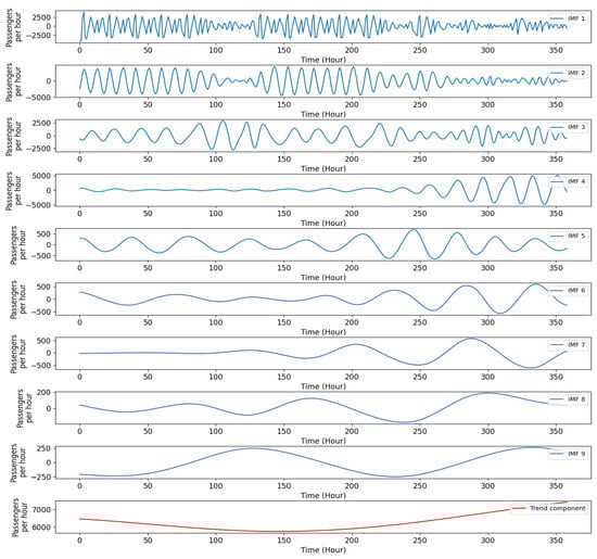
Figure 3. EMD of the time series of the Chunxi Road–Tianfu Square cross-sectional flow.

Table 3. Section flow time series.

Section Name	1	2	3	4	5	6	7	…
Cypress Field—LiaoJia Bay	248	708	538	352	232	181	174	…
LiaoJia Bay—Northern Trade Market	421	1386	992	564	364	269	298	…
Northern Trade Market—XingFu Bridge	486	1614	1122	653	462	460	504	…
…	…	…	…	…	…	…	…	…
ChunXi Road—TianFu Square	14,116	6636	4719	4597	4787	6076	5807	…

As can be seen from Table 4, the IMF instantaneous frequency of IMF1 and IMF2 in the time series represent short-term patterns, with cycles of about 1 h and 2 h, respectively. IMF3, IMF4, and IMF5 illustrate the peak hour modes, and the seasonal cycles are about 3.7 h, 6 h, and 9.3 h, respectively. IMF6, IMF7, and IMF8 stand for the daily service model, with seasonal cycles of about 13.6 h, 19.8 h, and 24 h, respectively. IMF9 describes a half-week service model with a seasonal cycle of about 50 h. The following two subsections will introduce how to fit and predict these components.

Table 4. IMF instantaneous frequency and cycle.

IMF	IMF1	IMF2	IMF3	IMF4	IMF5	IMF6	IMF7	IMF8	IMF9
$\mathrm{Frequency} {\omega }_i$	0.923	0.473	0.270	0.168	0.107	0.074	0.051	0.041	0.022
$\mathrm{Cycle} T_i$	1.082	2.117	3.699	5.963	9.340	13.58	19.76	24.15	49.06

4. Seasonal Components Prediction

The time series of the urban metro across-section passenger flow is split into two parts: the first part, the origin set, includes 60% of the data, and the rest, the test set, has 40% of the data. After removing the $r_i^n\left(t\right)$ from the original sequence, a difference series can be obtained, and it can be seen that the extremum points are basically distributed symmetrically around the zero-horizon line. Nine IMF functions decomposed from the first part’s data (the origin set) are fitted by the seasonal Fourier function, the parameters of which are shown in Table 5. The difference series and the addition of nine fitted seasonal Fourier functions are plotted in Figure 4. We can also see the forecasting periodic component predicted by the Fourier series in Figure 4.

Table 5. Parameters of the seasonal Fourier function.

	IMF1	IMF2	IMF3	IMF4	IMF5	IMF6	IMF7	IMF8	IMF9
$a_i$	260.7	−26.40	430.5	−563.8	1104	76.76	−3097	153.9	299.5
$b_i$	−200.6	−108.6	−349.4	−718.5	−442.7	87.33	1786	−793.2	161.4
$a_0$	−113.8

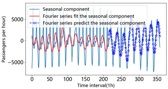
Figure 4. Fourier fitting function and predicting the seasonal part.

5. Trend Component Prediction

The trend component $R_i\left(t\right)$, which is the deterministic part of the urban metro sectional passenger flow, is the lowest frequency component obtained by EMD, and it is not affected by variations in the occasional commuting mode and can be fitted by spline interpolation. Based on Figure 5, the spline interpolation fitting of the remaining components and their predictions are pretty good.

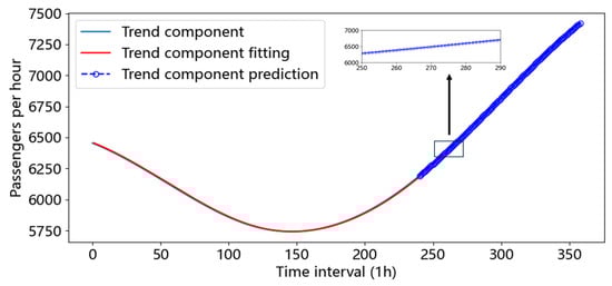
Figure 5. Fitting and prediction of spline interpolation components.

6. Prediction of Residual Component

In this section, we will introduce the architecture and modules of the STGCN-GAN model, including graphs of time convolutional networks and the training process of adversarial neural networks.

6.1. Definition of Predictive Model

From Equation (16), we obtain the residual component $V_i\left(t\right)$ and build a predictive model, as shown in Equation (23):

$$\left[{\hat{V}}_i(\overline{t}+1),{\hat{V}}_i(\overline{t}+2),\dots ,{\hat{V}}_i(\overline{t}+h)\right]=f\left(\left[V_i(\overline{t}-m+1),V_i(\overline{t}-m+2),\dots ,V_i\left(\overline{t}\right)\right];G\left(N,A\right);\vartheta \right)$$

(23)

where $\vartheta$ represents the argument to the function $f\left(·\right)$. Symbol $\overline{t}$ indicates the last item of the first part including 60% of the origin data. $G\left(N,A\right)$ represents the node graph structure of the metro system, and $N$ and $A$ represent the set of sections (or parking station or train maintenance base) and railway sections between two adjacent stations, respectively. $h$ represents the length of the predicted series, and m represents the length of the first part of the origin set. The crux of this equation is to use the observations of the previous m time intervals to predict the data for the $h$ time intervals in the future.

Forecasting passenger flow for all the cross-sections is a demanding task in terms of computational burden. There are a total of 352 cross-sections in the Chengdu urban metro network. Firstly, we calculate the average passenger flow of each cross-section in all periods, and then the cross-sections with the average passenger flow located in the first 40 percent are picked up, meaning 142 sections are selected, including 2 sections with the same average passengers flow. Finally, the Poisson correlation coefficient between the passenger flows of different two sections is calculated among these selected sections, which constitutes the correlation coefficient matrix ${\gamma }_{ij}$.

This defines the adjacency matrix $E\in R^{n\ast n}$, where each element $E_{ij}$ equals 0 if the correlation coefficient value ${\gamma }_{ij}$ is less than the threshold $\epsilon$; othervise, element $E_{ij}$ equals 1. In this study, the $\epsilon$ value is set as 0.75. $E_{ij}$ is defined as shown in Equation (24):

$$E_{ij}=\left\{\begin{array}{c}0, {\gamma }_{ij}<\epsilon \\ 1, {\gamma }_{ij}\ge \epsilon \end{array}\right.$$

(24)

6.2. The Architecture of the STGCN-GAN

The generator adopts a graph neural network STGCN to capture the spatial and temporal dependencies between nodes and generate future cross-sectional traffic. The discriminator also adopts a graph neural network GCN which takes two sets of samples generated by the generator STGCN and the corresponding true flow as inputs in order to determine which sample is real and which sample is false. The next section describes the components of the model in detail.

(a) The STGCN as a generator

The STGCN generator consists of two time–space blocks and an output layer. Each time–space block consists of two time domain convolutions and a spatial convolution. The output layer consists of a time convolutional layer and a fully connected layer, and a time domain convolutional block is shown in Figure 6.

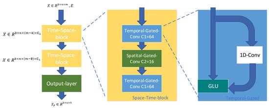
Figure 6. The architecture of the generator in detail.

The input and output of the generator: The network input is the vector $X\in R^{b\times n\times m}$ of the graph with b batch size; the $n$ dimension stands for the number of sections, and m time stands for steps. The network output is the feature vector $X_F\in R^{b\times n\times m}$ used to indicate the graph in the next m time steps.

Graph Convolutional Networks: In order to obtain complex spatial dependencies of urban rail sections, we use Graph Convolutional Networks (GCNs). The GCN recursion formula is defined as follows (25) [30]:

$${x_f}^{l+1}=\sigma \left(D^{-\frac{1}{2}}\hat{E}{D}^{-\frac{1}{2}}{x_f}^{l}W\right)$$

(25)

In Equation (25), each row ${x_f}^l\in R^{n\times m}$ of the matrix represents each section’s time series of cross-section traffic $\left[V_i(\overline{t}-m+1),V_i(\overline{t}-m+2),\dots ,V_i\left(\overline{t}\right)\right]$. “$\sigma \mathrm{”}$ is the sigmoid activation function. $E\in R^{n\times n}$ is the graph adjacency matrix. $\hat{E}\in R^{n\times n}$ can be calculated as $\hat{E}=E+I_n$. $I_n\in R^{n\times n}$ is the identity matrix. $D\in R^{n\times n}$ is the degree matrix of $\hat{E}$ and can be calculated as $D_{ii}={\sum }_j{\hat{E}}_{ij}$. $W\in R^{h\times m}$ stands for the weight matrix to be learned. Each row of the matrix ${x_f}^{l+1}$ represents the output with the prediction $[{\hat{V}}_i\left(\overline{t}+1\right),{\hat{V}}_i\left(\overline{t}+2\right),\dots ,{\hat{V}}_i\left(\overline{t}+h\right)]$ of each section.

Time–space blocks: The time domain convolutional layer contains $2{\mathrm{C}}_1$ convolution kernels $\mathsf{\Theta }\in R^{1\times k}$, and the input vector $X\in R^{b\times n\times m}$ is convolved along the time dimension. After performing GLU activation, the output $Y\in R^{b\times n\times \left(m-k+1\right)\times {\mathrm{C}}_1}$ is produced.

Spatial convolution is performed on the graph at each time step and contains $2{\mathrm{C}}_2$ convolution kernels $\mathsf{\Theta }\in R^{1\times 3}$. The input is $X\in R^{b\times n\times (m-k+1)\times {\mathrm{C}}_1}$, and the output is shown in (25). Namely, $Y=\sigma \left(D^{-\frac{1}{2}}\hat{E}{D}^{-\frac{1}{2}}XW\right)\in R^{b\times n\times (m-k+1)\times {\mathrm{C}}_2}$.

After a space–time convolutional block, the vector dimension and the time step dimension will be shortened 2 × (k − 1). So, after two space–time convolutional blocks, the vector becomes $X\in R^{b\times n\times (m-4\times (\mathrm{k}-1\left)\right)\times {\mathrm{C}}_1}$.

The output layer: The output layer consists of a time domain convolutional layer and a fully connected layer. The input vectors $X\in R^{b\times n\times (h-5\times (\mathrm{k}-1\left)\right)\times {\mathrm{C}}_1}$ reshaped into $X\in R^{b\times n\times (h-5\times (\mathrm{k}-1\left)\right)\times {\mathrm{C}}_1}$ are mapped through the fully connected layer $G\left(X\right)=WX+\theta , W\in R^{{\mathrm{C}}_1\times \left(m-5\times (\mathrm{k}-1)\right)\times h}$into $G\left(X\right)\in R^{b\times n\times h}$.

(b) The GCN as a discriminator

We use the GCN model as a discriminator to identify and learn characteristics of traffic data $X_R$. The discriminator input is the $G\left(X\right)\in R^{b\times n\times h}$ output of the generator or the real traffic for the corresponding period $X_R\in R^{b\times n\times h}$. The output of the discriminator is $p\in R^{1\times 1}$. We expect that if the input $X_R$ is real traffic data or close to real traffic data, the value of $D_{loss}$ is large; otherwise, $D_{loss}$ is small. The structure of the discriminator is shown in Figure 7, which depicts the GCN, self-attention mechanism, and fully connected layers, as well as the probability matrix The self-attention calculation mechanism is as follows (26)–(29):

$$X_{self\text{-}attention}=softmax(\frac{Q{K}^T}{d})V$$

(26)

$$Q=G\left(X\right)\ast W_{Q }or Q=X_R\ast W_{Q }$$

(27)

$$K=G\left(X\right)\ast W_{K }or K=X_R\ast W_{K }$$

(28)

$$V=G\left(X\right)\ast W_{V }or V=X_R\ast W_{V }$$

(29)

where $W_{Q },W_{K }{,W}_{V }\in R^{b\times n\times h}$ are all weight matrices; $Q,K,V$ is the result of the linear transformation of $G\left(X\right)$ or $X_R$. $X_{self\text{-}attention}\in R^{b\times n\times h}$ is the output of the self-attention layer. Then, we flatten $X_{self\text{-}attention}$into $X_{flatten}$ $\in R^{1\times h}$ and pass it through the weight matrix of the fully connected layer $W_{fc}\in R^{h\times 1}$ into $p\in R^{1\times 1}$.

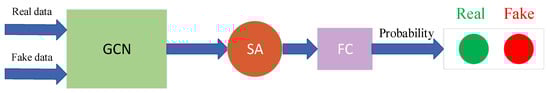
Figure 7. The architecture of the discriminator in detail.

6.3. Training Methodology

The parameters are updated with the gradient-decreasing loss functions of (23) and (24), where G and D are trained alternately until convergence. The training pseudocode for STGCN-GAN is shown in Table 6.

Table 6. The STGCN-GAN pseudocode.

Input: Normalized data  $\mathit{X}\in {\mathit{R}}^{\mathit{b}\times \mathit{n}\times \mathit{m}}$  Output:  $\mathit{G}\left(\mathit{X}\right)\in {\mathit{R}}^{\mathit{b}\times \mathit{n}\times \mathit{h}}$.

Setting: Generator and discriminator learning rate${\alpha }_G={\alpha }_D$= 0.005, batch size b = 10.

The Number of timesteps input $m$. The Number of timesteps output $h$. Initialization parameters ${\theta }_G, {\theta }_D$.

While not converged do:

for i in epoch:

Generate a random number r

A random batch $\mathit{X}\in R^{\mathit{b}\times \mathit{n}\times \mathit{m}}$ from real dataset which time period is $\left[\overline{t}-m+1,\overline{t}-m+2,\dots ,\overline{t}\right]$, $X_R\in R^{\mathit{b}\times \mathit{n}\times \mathit{h}}$ which time period is $\left[\overline{t}+1,\overline{t}+2,\dots ,\overline{t}+h\right]$

${\theta }_{G }\leftarrow {{\nabla }_{{\theta }_{G }}G}_{loss}=-\mathit{log}\left(1-D\left(G\left(X\right)\right)\right)$

Update the Generator G

${{\theta }_{D }\leftarrow \nabla }_{{\theta }_{D }} D_{loss}=-\mathit{log}\left(D\left(G\left(X\right)\right)\right)-\mathit{log}\left(1-D\left(X_R\right)\right)$

Update the Discriminator D

End while

Test environment: All experiments were compiled and tested on Python 3.9 (GPU: NVIDIA GeForce RTX 3070). All test results are based on the cross-sectional traffic data of the Chunxi Road–Tianfu Square flow (as an example).

After several rounds of training, it was found that the loss functions of both the generator and the discriminator converge to ln2, as shown in Figure 8, because the discriminator and generator loss functions are minimized under the conditions $D\left(G\left(X\right)\right)=D\left(X_R\right)=0.5$.

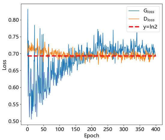
Figure 8. The loss functions of the generator and discriminator.

6.4. Residual Component Prediction Results and Analysis

(a) Baseline methods for comparison

To verify the predictive performance of the model proposed in this paper, we selected evaluation indicators such as mean absolute error (MAE) and root mean squared error (RMSE).

In order to verify the effectiveness of the proposed method, the following prediction methods were selected to compare their prediction effects with that of the proposed model: (1) Autoregressive Moving Average (ARIMA), (2) Long Short-Term Memory (LSTM), (3) Bi-directional Long Short-Term Memory (BiLSTM), (4) a spatio-temporal graph convolutional network (STGCN).The prediction effect is shown in Figure 9.

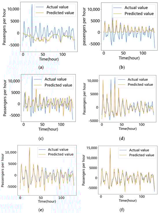
Figure 9. Visualizations of the prediction results derived from the different models: (a) ARIMA, (b) GCN, (c) LSTM, (d) BiLSTM, (e) STGCN, (f) STGCN-GAN.

Table 7 presents the evaluation index of the residual components of different models. It is clear that the traditional ARIMA model is inadequate for forecasting non-stationary time series. Although the GCN considered in this study can capture spatial information, it also performs poorly. We suspect that while the residual component is influenced by fluctuations in passenger flow, it is primarily related to time. The most successful predictors were Bi-LSTM, STGCN, and STGCN-GAN. The Bi-LSTM structure consists of two independent LSTMs that extract features from the input sequence in positive and reverse order. The Bi-LSTM model aims to incorporate information from both past and future time series into the feature data obtained at each time point. The experimental results indicate that this model outperforms single LSTM models in capturing the characteristics of previous time series.

Table 7. Comparison of the indicators of the residual components predicted by different models.

Models	MAE	RMSE	STGCN-GAN Boost (MAE/RMSE)
ARIMA	1719.6	1970.2	(52%/45%)
GCN	1114.7	1379.4	(28%/21%)
LSTM	1493.2	1847.0	(46%/41%)
Bi-LSTM	1022.5	1173.0	(27%/9%)
STGCN	918.2	1145.2	(12%5%)
STGCN-GAN	802.3	1085.2	----

However, when considering passenger flow on metro lines, STGCN-GAN outperforms Bi-LSTM, with STGCN-GAN being the best performer overall, improving MAE performance by 27% and RMSE performance by 9% compared to Bi-LSTM.

In addition, we also tried to experiment with other neural networks as discriminators, and the results are shown in Table 8 below: In addition to a GCN, MLP works best as a discriminator, but there are disadvantages, as the training is unstable, and the generator and discriminator can never achieve equilibrium results. The MLP loss function is shown in Figure 10.

Table 8. Comparison of the performance of different models as discriminators.

Models	MAE	RMSE	GCN Boost (MAE/RMSE)
GAT	1204.5	1571.5	(33%/31%)
CNN	1368.7	1123.4	(41%/3%)
LSTM	2165.2	3217.0	(65%/65%)
MLP	862.1	1145.2	(7%/5%)
GCN	802.3	1085.2	-----

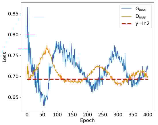
Figure 10. Using MLP as a discriminator led to GD training loss.

(b) Ablation study

To verify the effect of EMD on prediction accuracy, we added a model without EMD as a baseline model. The prediction performance results are shown in Table 9, which depicts a comparison of the results achieved by the temporal models and hybrid models.

Table 9. Comparison of the results achieved by the temporal models and hybrid models.

	Models	MAE	RMSE
Without any decomposition	ARIMA	2297.0	2211.8
	GCN	1782.1	1911.2
	LSTM	1835.2	2424.0
	Bi-LSTM	1590.8	2042.6
	STGCN	1360.4	1731.2
	STGCN-GAN	1112.6	1406.6
With EMD	ARIMA	1719.6	1970.2
	GCN	1114.7	1379.4
	LSTM	1493.2	1847.0
	Bi-LSTM	1022.5	1673.0
	STGCN	918.2	1245.2
	STGCN-GAN	802.3	1085.2
With CEEMDAN decomposition	ARIMA	4669.8	5690.7
	GCN	3114.7	1379.4
	LSTM	2165.4	1457.0
	Bi-LSTM	1524.6	2068.0
	STGCN	1582.5	2249.7
	STGCN-GAN	1502.3	2085.1

We noticed that all models achieved improved performance with EMD-based decomposition. The increase is about 15–20%. However, when using CEEMDAN decomposition, the prediction performance becomes worse than it originally was. Our guess is that CEEMDAN may have overdecomposed the signal, dissolving noise or irrelevant patterns into the IMFs as well. These additional patterns can interfere with predictions, making them more complex and less accurate.

(c) Time cost analysis

From Figure 11, we can see that predicting the residual components took about 80% of the time for the hybrid model, mainly because deep learning training involves high hardware requirements and long training times. In contrast, EMD did not take too long. EMD brings a significant improvement in predictive performance because EMD can, to a certain extent, remove noise from the data, allowing the neural network to make better predictions. Compared with Bi-LSTM, graph neural networks take longer to train because Bi-LSTM trains a single sequence, while graph neural networks train multidimensional sequences, but models that consider cross-sectional spatiotemporal correlations predict better. STGCN-GAN is acceptable, despite a slight increase in time cost, because of its guaranteed improved performance. The detailed forecast time of each part is shown in Table 10.

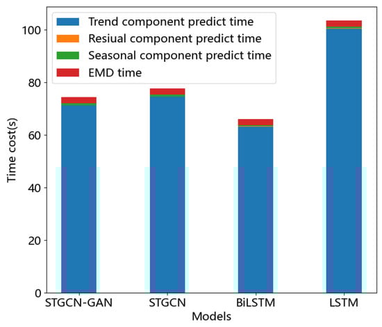
Figure 11. Time cost values for the different models.

Table 10. Time cost values for the different models.

Models	EMD	Seasonal Component	Trend Component	Resiual Component
STCGN-GAN	2.4 s	0.7 s	0.05 s	71.2 s
STCGN	2.4 s	0.7 s	0.04 s	74.6 s
Bi-LSTM	2.4 s	0.7 s	0.08 s	63.2 s
LSTM	2.4 s	0.7 s	0.12 s	100.4 s

(d) Analysis of the number of trains running

However, it is not enough to predict cross-sectional flow; cross-sectional flow forecasting needs to provide a valuable reference for train demand forecasting. Based on the prediction of cross-sectional flow, we can predict the number of trains required per hour on each line, which can be calculated as shown in (30):

$$N_{least}=\min (\max \left(\frac{N_{max}}{\beta N_C},\frac{3600}{T_{max}}\right),\frac{3600}{T_{min}})$$

(30)

In this formula, $N_{least}$ refers to the number of trains in different periods, $N_{max}$ refers to the maximum cross-sectional flow in the line, and $N_C$ refers to the maximum capacity of train; according to the Chengdu metro train model, the $N_C$ is about 1500. $\beta$ refers to the full load factor, which is set as 0.9. $T_{min}$ refers to the minimum departure interval, which is about 90 s. $T_{max}$ refers to the maximum departure interval, which is regarded as 600 s.

According to Formula (28), the figure for calculating the number of trains required to run on each line and the diagonal error is shown in Figure 12.

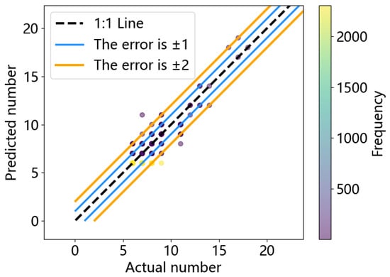
Figure 12. Diagonal error plot of train demand.

Based on Figure 12 and Figure 13, the error of predicting train demand is controlled within 2, and the prediction accuracy is about 95%.And the prediction accuracy of the STGCN-GAN model is better than that of the other baseline models. However, it can be seen that the main error sources in the three models are the same as the flat-peak period and the low-peak period, and in the future, we will study the passenger flow synergy of multiple traffic modes to avoid wasting resources.

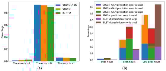
Figure 13. (a) The proportion of train errors in the top three forecasting methods; (b) statistics on the sources of the errors at different periods.

7. Conclusions and Future Work

In this paper, the Chengdu Metro’s across-section traffic flow was predicted by using a hybrid prediction method named STGCN-GAN, which is based on a combination of EMD and a graph convolutional neural network. The STGCN-GAN method predicts the residual component better than other baseline models, and the improvement range is between 15% and 50%. It also predicted the number of trains on different lines per hour in the next 7 days with an accuracy rate of about 95%. Although our proposed method has achieved significant improvements in some aspects, we should also note its limitations. In our experiments, we observed a 10% increase in computation time. Future work could explore the possibility of further optimizing the algorithm to reduce computation time while maintaining stability in terms of model performance, and we will work on the coordination of passenger flow control in multiple modes of transportation.

References

- Ortúzar, J.d.D. Future transportation: Sustainability, complexity and individualization of choices. Commun. Transp. Res. 2021, 1, e100010. [Google Scholar] [CrossRef]
- Hussain, E.; Bhaskar, A.; Chung, E. Transit OD matrix estimation using smartcard data: Recent developments and future research challenges. Transp. Res. Part C Emerg. Technol. 2021, 125, 103044. [Google Scholar] [CrossRef]
- Wang, X.; Kang, Y.; Hyndman, R.J.; Li, F. Distributed ARIMA models for ultra-long time series. Int. J. Forecast. 2022, 39, 1163–1184. [Google Scholar] [CrossRef]
- Zhao, J.; Yu, Z.; Yang, X.; Gao, Z.; Liu, W. Short term traffic flow prediction of expressway service area based on STL-OMS. Phys. A Stat. Mech. Its Appl. 2022, 595, 126937. [Google Scholar] [CrossRef]
- Lin, G.; Lin, A.; Gu, D. Using support vector regression and K-nearest neighbors for short-term traffic flow prediction based on maximal information coefficient. Inf. Sci. 2022, 608, 517–531. [Google Scholar] [CrossRef]
- Zhao, J.; Yan, Z.; Chen, X.; Han, B.; Wu, S.; Ke, R. k-GCN-LSTM: A k-hop Graph Convolutional Network and Long–Short-Term Memory for ship speed prediction. Phys. A Stat. Mech. Its Appl. 2022, 606, 128107. [Google Scholar] [CrossRef]
- Yu, B.; Lee, Y.; Sohn, K. Forecasting road traffic speeds by considering area-wide spatio-temporal dependencies based on a graph convolutional neural network (GCN). Transp. Res. Part C Emerg. Technol. 2020, 114, 189–204. [Google Scholar] [CrossRef]
- Lee, K.; Rhee, W. DDP-GCN: Multi-graph convolutional network for spatiotemporal traffic forecasting. Transp. Res. Part C Emerg. Technol. 2022, 134, 103466. [Google Scholar] [CrossRef]
- Yang, H.-F.; Chen, Y.-P.P. Hybrid deep learning and empirical mode decomposition model for time series applications. Expert Syst. Appl. 2019, 120, 128–138. [Google Scholar] [CrossRef]
- Liu, Y.; Wu, F.; Liu, Z.; Wang, K.; Wang, F.; Qu, X. Can language models be used for real-world urban-delivery route optimization? Innovation 2023, 4, 100520. [Google Scholar] [CrossRef] [PubMed]
- Tselentis, D.I.; Vlahogianni, E.I.; Karlaftis, M.G. Improving short-term traffic forecasts: To combine models or not to combine? IET Intell. Transp. Syst. 2015, 9, 193–201. [Google Scholar] [CrossRef]
- Zhang, Y.; Zhang, Y.; Haghani, A. A hybrid short-term traffic flow forecasting method based on spectral analysis and statistical volatility model. Transp. Res. Part C Emerg. Technol. 2014, 43, 65–78. [Google Scholar] [CrossRef]
- Mao, Y.; Yu, X. A hybrid forecasting approach for China’s national carbon emission allowance prices with balanced accuracy and interpretability. J. Environ. Manag. 2023, 351, 119873. [Google Scholar] [CrossRef]
- Huang, H. Introduction to the HILBERT–HUANG Transform And Its Related MathmaticalL Problems. Hilbert Huang Transform. Its Appl. 2003, 1–26. [Google Scholar] [CrossRef]
- Wei, Y.; Chen, M.-C. Forecasting the short-term metro passenger flow with empirical mode decomposition and neural networks. Transp. Res. Part C Emerg. Technol. 2012, 21, 148–162. [Google Scholar] [CrossRef]
- Yu, X.; Shi, S.; Xu, L. A spatial–temporal graph attention network approach for air temperature forecasting. Appl. Soft Comput. 2021, 113, 107888. [Google Scholar] [CrossRef]
- He, K.; Chen, Y.; Tso, G.K.F. Price forecasting in the precious metal market: A multivariate EMD denoising approach. Resour. Policy 2017, 54, 9–24. [Google Scholar] [CrossRef]
- Cao, J.; Li, Z.; Li, J. Financial time series forecasting model based on CEEMDAN and LSTM. Phys. A Stat. Mech. Its Appl. 2019, 519, 127–139. [Google Scholar] [CrossRef]
- Huang, Y.; Hasan, N.; Deng, C.; Bao, Y. Multivariate empirical mode decomposition based hybrid model for day-ahead peak load forecasting. Energy 2022, 239, 122245. [Google Scholar] [CrossRef]
- Hao, W.; Sun, X.; Wang, C.; Chen, H.; Huang, L. A hybrid EMD-LSTM model for non-stationary wave prediction in offshore China. Ocean Eng. 2022, 246, 110566. [Google Scholar] [CrossRef]
- Song, C.; Chen, X.; Wu, P.; Jin, H. Combining time varying filtering based empirical mode decomposition and machine learning to predict precipitation from nonlinear series. J. Hydrol. 2021, 603, 126914. [Google Scholar] [CrossRef]
- Duan, J.-H.; Li, W.; Zhang, X.; Lu, S. Forecasting fine-grained city-scale cellular traffic with sparse crowdsourced measurements. Comput. Netw. 2022, 214, 109156. [Google Scholar] [CrossRef]
- Wu, G.; Zhang, J.; Xue, H. Long-Term Prediction of Hydrometeorological Time Series Using a PSO-Based Combined Model Composed of EEMD and LSTM. Sustainability 2023, 15, 13209. [Google Scholar] [CrossRef]
- Chen, M.-C.; Wei, Y. Exploring time variants for short-term passenger flow. J. Transp. Geogr. 2011, 19, 488–498. [Google Scholar] [CrossRef]
- Huang, H.; Chen, J.; Sun, R.; Wang, S. Short-term traffic prediction based on time series decomposition. Phys. A Stat. Mech. Its Appl. 2022, 585, 126441. [Google Scholar] [CrossRef]
- Goodfellow, I. Generative Adversarial Nets. In Proceedings of the Advances in Neural Information Processing Systems 27, Montreal, QB, Canada, 8–13 December 2014; pp. 2672–2680. [Google Scholar]
- Khaled, A.; Elsir, A.M.T.; Shen, Y. TFGAN: Traffic forecasting using generative adversarial network with multi-graph convolutional network. Knowl. Based Syst. 2022, 249, 108990. [Google Scholar] [CrossRef]
- Zhang, L.; Wu, J.; Shen, J.; Chen, M.; Wang, R.; Zhou, X.; Xu, C.; Yao, Q.; Wu, Q. SATP-GAN: Self-attention based generative adversarial network for traffic flow prediction. Transp. B Transp. Dyn. 2021, 9, 552–568. [Google Scholar] [CrossRef]
- Zhou, K.; Wang, W.; Huang, L.; Liu, B. Comparative study on the time series forecasting of web traffic based on statistical model and Generative Adversarial model. Knowl. Based Syst. 2021, 213, 106467. [Google Scholar] [CrossRef]
- Thomas, K. Semi-Supervised Classification with Graph Convolutional Networks. In Proceedings of the 5th International Conference on Learning Representations, Toulon, France, 24–26 April 2017; p. 14. [Google Scholar]
Disclaimer/Publisher’s Note: The statements, opinions and data contained in all publications are solely those of the individual author(s) and contributor(s) and not of MDPI and/or the editor(s). MDPI and/or the editor(s) disclaim responsibility for any injury to people or property resulting from any ideas, methods, instructions or products referred to in the content. |
© 2024 by the authors. Licensee MDPI, Basel, Switzerland. This article is an open access article distributed under the terms and conditions of the Creative Commons Attribution (CC BY) license (https://creativecommons.org/licenses/by/4.0/).