Abstract
Accurate prediction of spatial variation in water quality in small microwaters remains a challenging task due to the complexity and inherent limitations of the optical properties of small microwaters. In this paper, based on unmanned aerial vehicles (UAV) multispectral images and a small amount of measured water quality data, the performance of seven intelligent algorithm-optimized SVR models in predicting the concentration of chlorophyll (Chla), total phosphorus (TP), ammonia nitrogen (NH3-N), and turbidity (TUB) in small and micro water bodies were compared and analyzed. The results show that the Gray Wolf optimized SVR model (GWO-SVR) has the highest comprehensive performance, with R2 of 0.915, 0.827, 0.838, and 0.800, respectively. In addition, even when dealing with limited training samples and different data in different periods, the GWO-SVR model also shows remarkable stability and portability. Finally, according to the forecast results, the influencing factors of water pollution were discussed. This method has practical significance in improving the intelligence level of small and micro water body monitoring.
1. Introduction
Small inland water bodies are critical to agricultural production, ecosystem maintenance, and the livelihood of local communities [1]. However, due to rapid social development, excessive land development, and improper management of water resources, these water bodies face different degrees of pollution threats. Pollution not only affects water quality and ecosystem health but also threatens people’s water safety and health [2]. Therefore, accurate water quality monitoring is very important for controlling and reducing water pollution, maintaining ecological balance, and promoting sustainable development [3].
Traditional water quality monitoring methods, such as manual sampling and automated monitoring stations, are limited to point-scale measurements [4]. These approaches, with accuracy at specific locations, are expensive, time-consuming, and insufficient for capturing the continuous spatial and temporal changes in river water quality [5]. In addition, these methods lack comprehensive insights into pollutant source control [6,7].
Remote sensing technology has been applied to water quality monitoring and assessment of oceans, lakes, and rivers, which addresses the limitations of traditional monitoring with narrow observation scales or temporal discontinuities [8]. Early qualitative analysis of water quality in large-scale waters mainly used low- and medium-resolution satellite sensors [9]. Subsequently, high-resolution sensors for water quality monitoring such as Landsat series and Sentinel 2 A/B multispectral instruments are widely used worldwide [10,11,12]. However, the limited accuracy of satellites and the long revisit cycle of satellites led to the inability to efficiently and accurately assess small-sized water bodies [13]. In recent years, unmanned aerial vehicles (UAVs) have been successfully used for water monitoring due to their flexibility, low cost, and high resolution. For instance, Castro et al. compared the performance of satellite and UAV remote sensing in the detection of Chla concentration in small reservoirs and they found that the Chla concentration detection based on UAV remote sensing is more accurate [14].
The principle of UAV-based water quality monitoring is to use sensors combined with drones to capture spectral information from the water body. The obtained spectral data are subsequently processed using optical models and advanced data analysis techniques to derive accurate concentration values for a variety of water quality parameters [15]. However, research on water quality monitoring in small-sized rivers using remote sensing was still limited. Current studies primarily focus on larger bodies of water, with relatively less attention given to small streams [16]. Especially small-micro bodies of water located in typical agricultural areas, these small-micro bodies have limited surface area, making them highly susceptible to external influences from agricultural activities and residential living. The water quality composition is complex, with significant variations and pollution sources being challenging to control effectively [17]. The optical characteristics of the water exhibit nonlinear, multivariate, and non-normal distributions [18]. Traditional linear regression models (LRM) are only capable of addressing linear relationships and struggle to handle the complex nonlinear relationships present in the water quality monitoring of small-micro bodies [19,20]. Simultaneously, owing to the relatively difficult acquisition of ground real water quality data of small-micro bodies, there is a lack of sufficient data as training samples, so it is necessary to adopt advanced models or algorithms that can show good performance under a small amount of water quality data, for example, machine learning algorithms.
Currently, machine learning (ML) methods have advantages in dealing with nonlinear relationships and high-dimensional data [21]. Support vector machine regression (SVR), a prominent machine learning algorithm, exhibits extensive application in water quality inversion. The SVR model well adapts to the real situation and provides more accurate prediction results by automatically learning patterns and correlations in the data without making any assumptions about the data distribution. This holds even when handling small sample sizes, demonstrating strong performance [22]. Despite many advantages of SVR, there are still some limitations in inversion models, and the choice of parameters has a large impact on the results. Inappropriate parameter selection may lead to underfitting or overfitting, and different parameter settings could result in significant differences in performance [23,24,25]. Various optimization algorithms have been used to optimize the SVR and further improve the inversion accuracy of water quality parameters, e.g., Gray Wolf Optimizer Algorithm (GWO) [26], Genetic Algorithm (GA) [27], Particle Swarm Optimization Algorithm (PSO) [28], Ant Colony Optimization algorithm (ACO) [29], Firefly Algorithm (FA) [30], Sparrow Search Algorithm (SSA) [31], Hunter–Prey Algorithm (HPO) [32], etc. These optimization algorithms can search for the optimal solution in the parameter space and help to adjust the parameters of the SVR model, thus improving the inversion accuracy.
At present, for small-micro water bodies with dispersed pollution and complex spectral information, an ideal model that can effectively predict water quality parameters in the case of limited samples has not been retrieved [33]. In this paper, by combining the multispectral data collected by UAV with the ground monitoring data, the algorithm of SVR is optimized and the prediction model of river Chla, NH3-N, TP, and TUB concentrations is constructed. This paper aims to provide an effective scientific method to monitor and predict the water quality of small and micro rivers. The main research contents of this paper include (1) enhancing the relationship between water quality parameters and unmanned aerial vehicle multispectral data through a band combination approach; (2) comparing the performance of SVR optimization in water quality concentration inversion synthesis by different optimization algorithms and selecting the optimal inversion model; (3) verifying the stability and generalization of the optimal model with a small number of samples and at different times; and (4) exploring the spatial distribution characteristics of Chla, TP, NH3-N, and TUB concentrations in the study area. The influence elements were analyzed to provide a scientific basis for pollutant source tracing and management.
2. Materials and Methods
2.1. Study Area
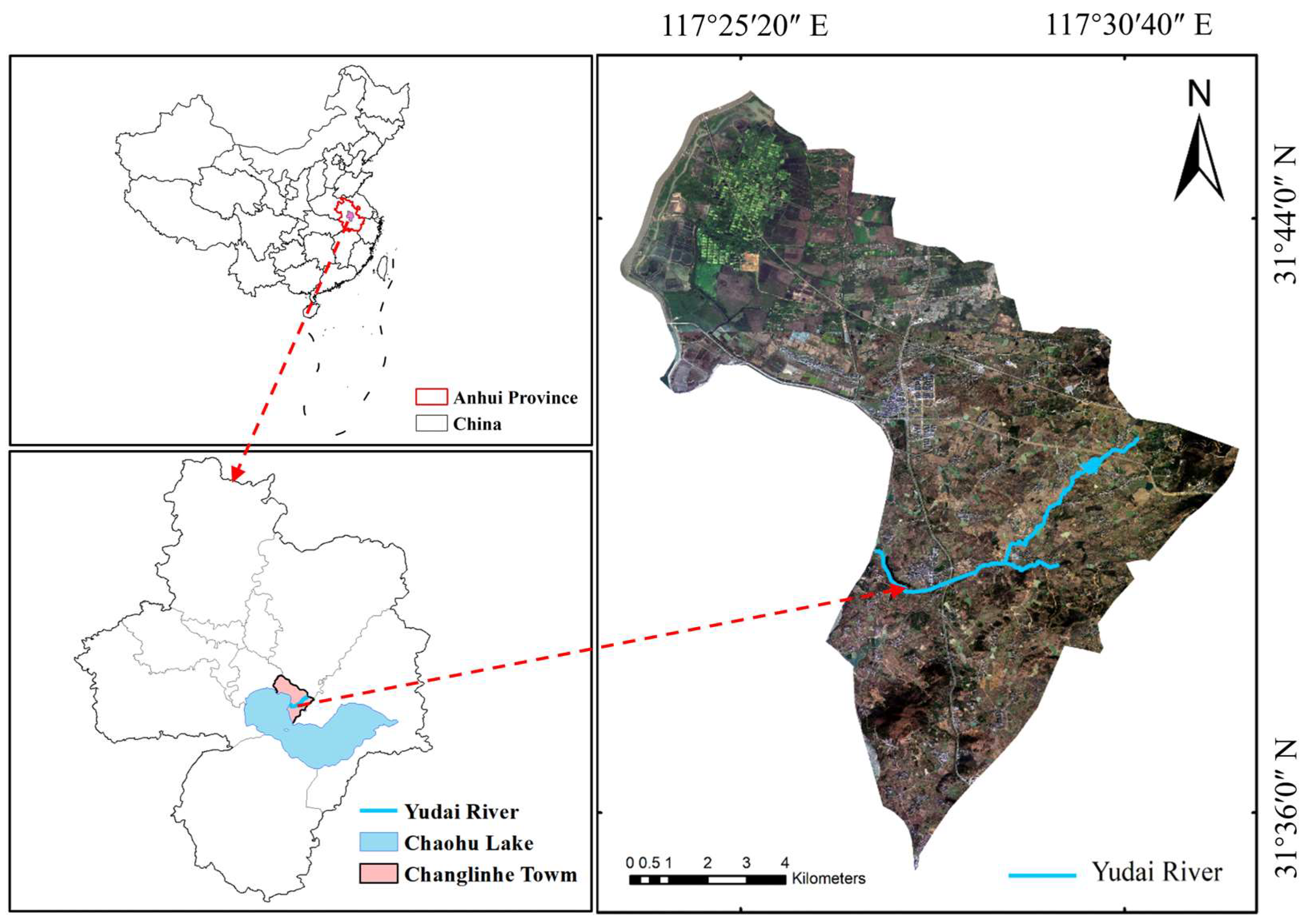
The selected minor tributary Yudai River was located in Feidong County, Hefei City, Anhui province of China, with geographic co-ordinates ranging from 31°34′ to 32°16′ N and 117°19′ to 117°52′ E selected as the study area. This river is a typical closed water body, which was mainly influenced by surrounding drainages and rainfall.
This work mainly focuses on the lower reaches of the Yudai River with a maximum width of no more than 15 m and the narrowest width of only 2 m. The length of the river is approximately 3.43 km with its drainage area 0.68 km2. The downstream area primarily encompasses the market town and agricultural planting zones, where the sewage network infrastructure is insufficient currently, resulting in difficulties in effectively treating domestic sewage. Potential sources of pollution in this area may include nutrient (N and P) runoff from agricultural activities, wastewater discharge from fisheries, domestic sewage, and livestock manure from rural farming. The sewage produced by the pollution source finally flows into Chaohu Lake and becomes one of the pollution sources of Chaohu Lake (Figure 1).
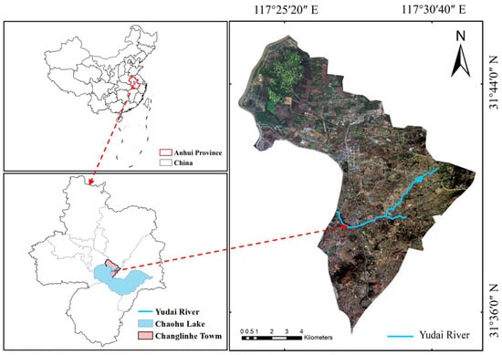
Figure 1.
Location of the lower reaches of the Yudai River.
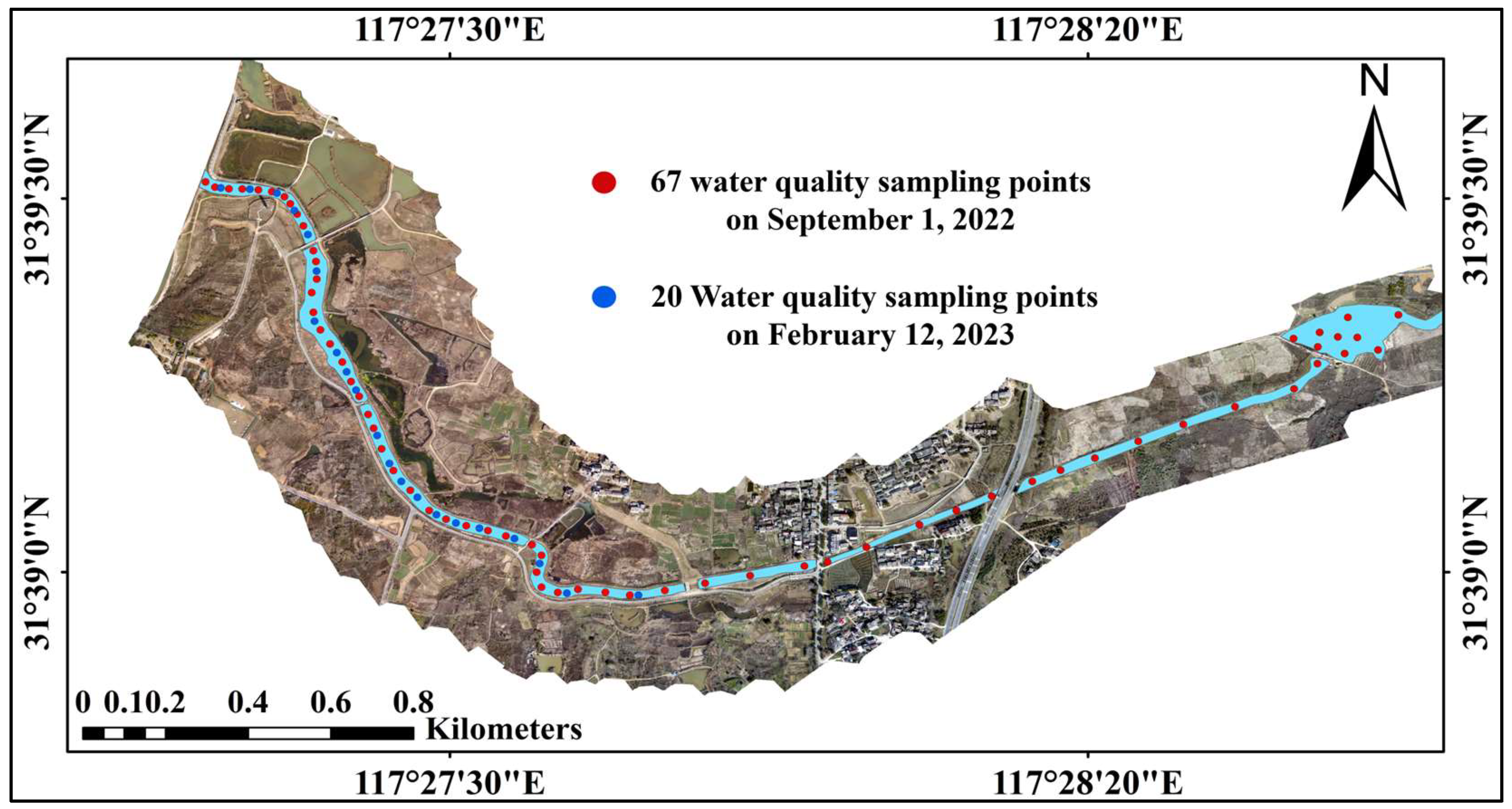
2.2. Water Sample Collection and Water Quality Parameter Determination
The collection of river water samples was concurrently coordinated with UAV flights. Sampling points were positioned in the central region of the river at regular intervals of 80–120 m, ensuring uniform collection and full reflection about the water quality of the river (Figure 2). Meanwhile, a real-time positioning system (A8, Zhuolin Technology, Hefei, China) was used to record the latitudes and longitudes of each sample site. Water samples (1.0 L) were obtained at each sampling point from a depth of 0 to 0.5 m. The water samples were then evenly collected into two different bottles. One bottle was supplemented with 1 mL of magnesium carbonate (MgCO3) suspension to prevent any potential dissolution of pigments caused by acidification. The other bottle was pretreated with sulfuric acid (18.4 mol/L) to ensure a pH lower than 2.0. A total of four water quality indicators, i.e., TP, Chla, NH3-N, and TUB, were determined. Among four water quality indicators, Chla and TUB were tested on the same day of sampling and NH3-N and TP were tested within 72 h in the laboratory (Table S1). Sampling procedures were strictly by Chinese water quality sampling standards (Water Quality—Guidance on sampling techniques HJ494-2009 [34]).
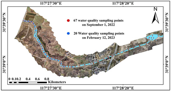
Figure 2.
Distribution of sampling points.
2.3. UAV Image Acquisition and Preprocessing
The Genie 4 multispectral UAV (P4M, Shenzhen, Guangdong, China) was used as the data acquisition tool in the current study. The UAV is equipped with an all-in-one multispectral imaging system that includes a visible camera and five multispectral cameras. These cameras have a resolution of 2 megapixels and a global shutter function. The imaging system, mounted on a three-axis gimbal, could provide clear and stable imaging and acquires multispectral images in five bands: blue (B1), green (B2), red (B3), eed-edge (B4), and near-red (B5). Moreover, to mitigate the influence of ambient light during data acquisition, an integrated multispectral light intensity sensor was positioned atop the setup.
The UAV was subjected to uncontrollable factors during the flight, which may lead to geometric and radiometric distortions in the images. Therefore, the raw images were pre-pretreated (including band alignment, orthophoto mosaic, radiometric correction, and reflectance calculation) before being used to ensure the accuracy and comparability of the data [35,36,37].
This study involved two experimental sample acquisitions on 1 September 2022 and 12 February 2023 (Table 1). The data collection process was conducted under favorable conditions (clear weather, calm winds, and excellent visibility) to guarantee the reliability and accuracy of the data.

Table 1.
UAV flight parameters.
2.4. The Intelligent-Algorithm-Optimized SVR Algorithm
The SVR model was established and combined with seven hyperparametric optimization methods to perform model optimization. Through the formulation of a multitude of feature combinations exhibiting strong correlations, the precision of the model for river water quality inversion is augmented (Figure 3). This method can be applied to small river water quality inversion problems based on UAV multi-spectrum and has a certain reference value in practical application.
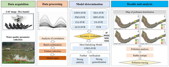
Figure 3.
Water quality parameter inversion model flowchart.
2.4.1. SVR Model
SVR is a support vector machine (SVM)-based regression algorithm for solving linear or nonlinear regression problems. The central tenet of SVR is to construct an optimal hyperplane in a high-dimensional space so that the distance from the hyperplane to the training samples is as small as possible and the error does not exceed a certain tolerance [38].
The essence of the SVR algorithm lies in the manipulation of training data, involving the transformation of data into a high-dimensional space and the identification of an optimal hyperplane within this space. The model training process of SVR can be represented as a convex optimization problem, whose objective is to minimize the loss function while satisfying the constraints of the support vector. Commonly used loss functions include linear loss function, square loss function, and absolute value loss function. After the training is completed, SVR performs regression prediction by calculating the distance from the test data points to the optimal hyperplane [39,40,41].
The optimization problem of SVR can be expressed in the following form:
where is the weight vector, C is the regularization parameter, is the complexity-related term, the relaxation variable, is the mapping function, and is the loss function. The objective function (1) consists of two components: a regularization term 1/2 to control the complexity of the model and an error term to measure the prediction error. Constraints (2) and (3) restrict the difference between the predicted and true values to within ε and relax these constraints by the slack variables. The goal of the final SVR is to find a prediction function , such that the sum of the objective function and the error term is minimized while satisfying the tolerance limits. b is the threshold value.
2.4.2. Algorithm Optimization
In this study, seven optimization algorithms, i.e., GWO, GA, PSO, ACO, FA, SSA, and HPO, were employed to optimize the SVR model and enhance its predictive performance. Modeling and forecasting were carried out using the Python programing language (Python 3.6).
- (1)
- Gray Wolf Optimization (GWO)
GWO is a swarm intelligence-based optimization algorithm. It simulates the collaborative behavior of a gray wolf pack to solve optimization problems. GWO achieves a balance between global exploration and local exploitation, resulting in effective and efficient optimization. The population size is set to 20, the maximum number of iterations is 100, and the convergence factor is set to 2 [42].
- (2)
- Genetic Algorithm (GA)
GA is an efficient optimization algorithm based on genetics and natural selection. It finds the optimal solution by simulating the process of natural evolution through genetic operations. The population size is set to 20 and the maximum number of iterations is 100 [43,44,45].
- (3)
- Particle Swarm Optimization (PSO)
PSO is a population-based optimization algorithm that uses a swarm of particles to search for the optimal solution in a multidimensional space. It efficiently solves complex optimization problems and provides high performance and accuracy. In this study, the population size is set to 20, the maximum number of iterations is 100, and the individual learning factor and social learning factor are set to 1.5 [46,47,48].
- (4)
- Ant Colony Optimization (ACO)
ACO is an ant-inspired optimization algorithm that uses pheromones and positive feedback to find the shortest path. It is adaptive, efficient, and widely used in solving complex optimization problems. The population size is set to 20, the maximum number of iterations is 100, the transfer probability constant is 0.2, and the pheromone evaporation coefficient is 0.9 [49,50].
- (5)
- Firefly Algorithm (FA)
FA is a swarm-based optimization algorithm inspired by firefly behavior. It efficiently solves complex optimization problems by attracting individuals toward brighter solutions. The population size is set to 20, the maximum number of iterations is 100, the phototaxis coefficient is 0.000001, and the maximum attractiveness is 1 [51,52].
- (6)
- Sparrow Search Algorithm (SSA)
SSA is a swarm intelligence optimization algorithm inspired by sparrows’ foraging behavior. It utilizes discoverers and followers to optimize food acquisition efficiency through collaboration. The population size is set to 20 and the maximum number of iterations is 100 [53,54].
- (7)
- Hyperparameter optimization (HPO)
HPO is an optimization algorithm inspired by the competitive and co-operative relationship between hunters and prey in nature. It is effective for complex optimization problems, offering global search and convergence. The maximum number of iterations is set to 100 and the tuning parameter is set to 0.1 [55,56].
2.5. Model Accuracy Assessment
Four metrics were employed in the model accuracy assessment, i.e., determination (R2), root mean square error (RMSE), mean square error (MSE), and mean absolute error (MAE). R2 assesses the goodness-of-fit of the regression model, with values closer to 1 indicating higher predictive ability. RMSE and MSE measure the deviation between the predicted and the measured value, with lower values indicating higher prediction accuracy of the model. MAE quantifies the average magnitude of errors between predicted and measured values.
where is the measured value, is the predicted value, n represents the number of samples in the dataset, and is the mean value of the measured concentration.
3. Results
3.1. Split of Dataset
A total of 67 samples were collected and four water quality parameters were determined (Table 2). A random sampling approach was employed to partition the entire dataset into a training set (including 50 samples) and a test set (including 17 samples), with a ratio of about 3:1.
Table 2.
The measured concentrations of four water quality parameters.
3.2. Selection of Highly Sensitive Features as Model Inputs
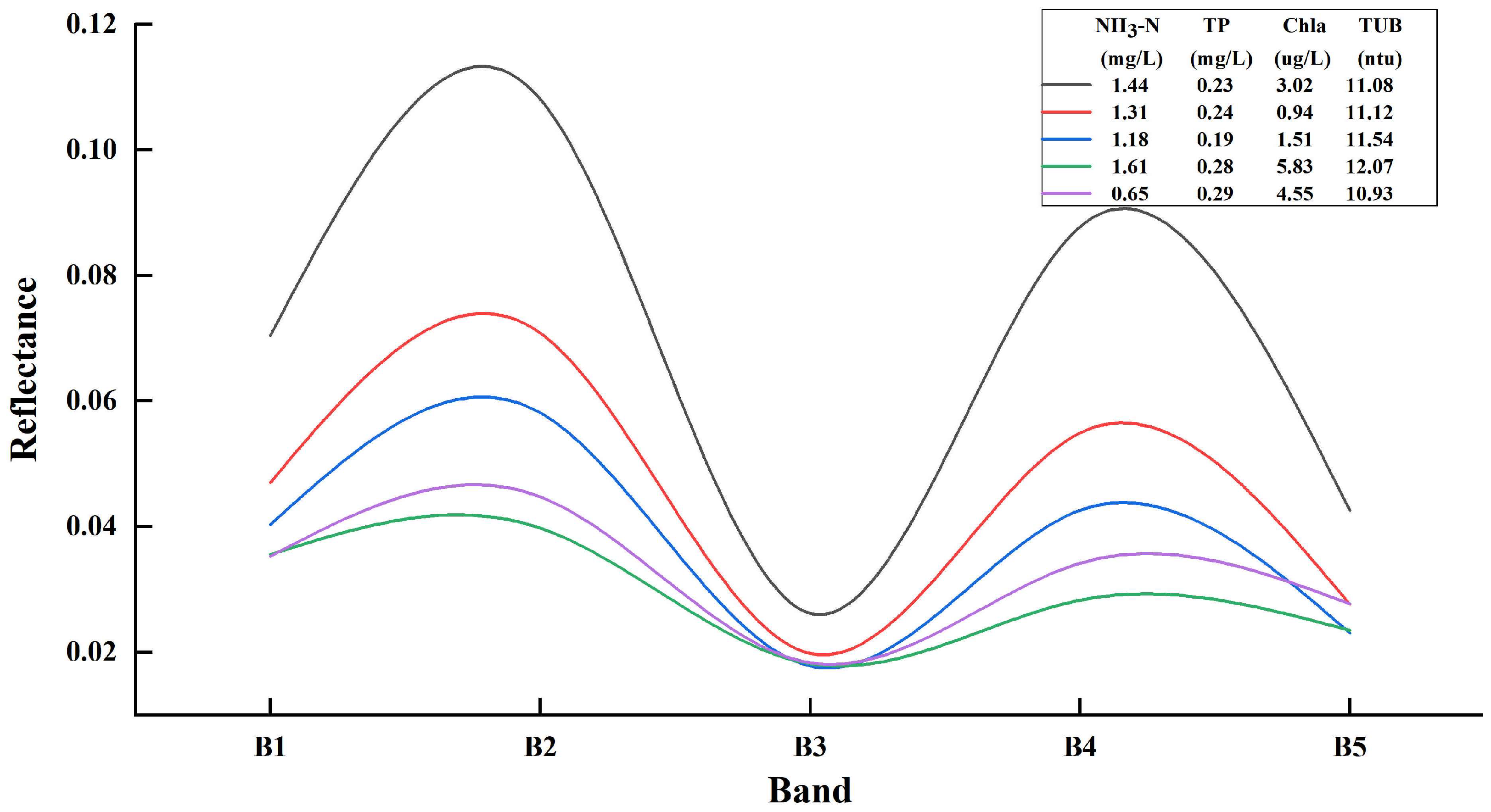
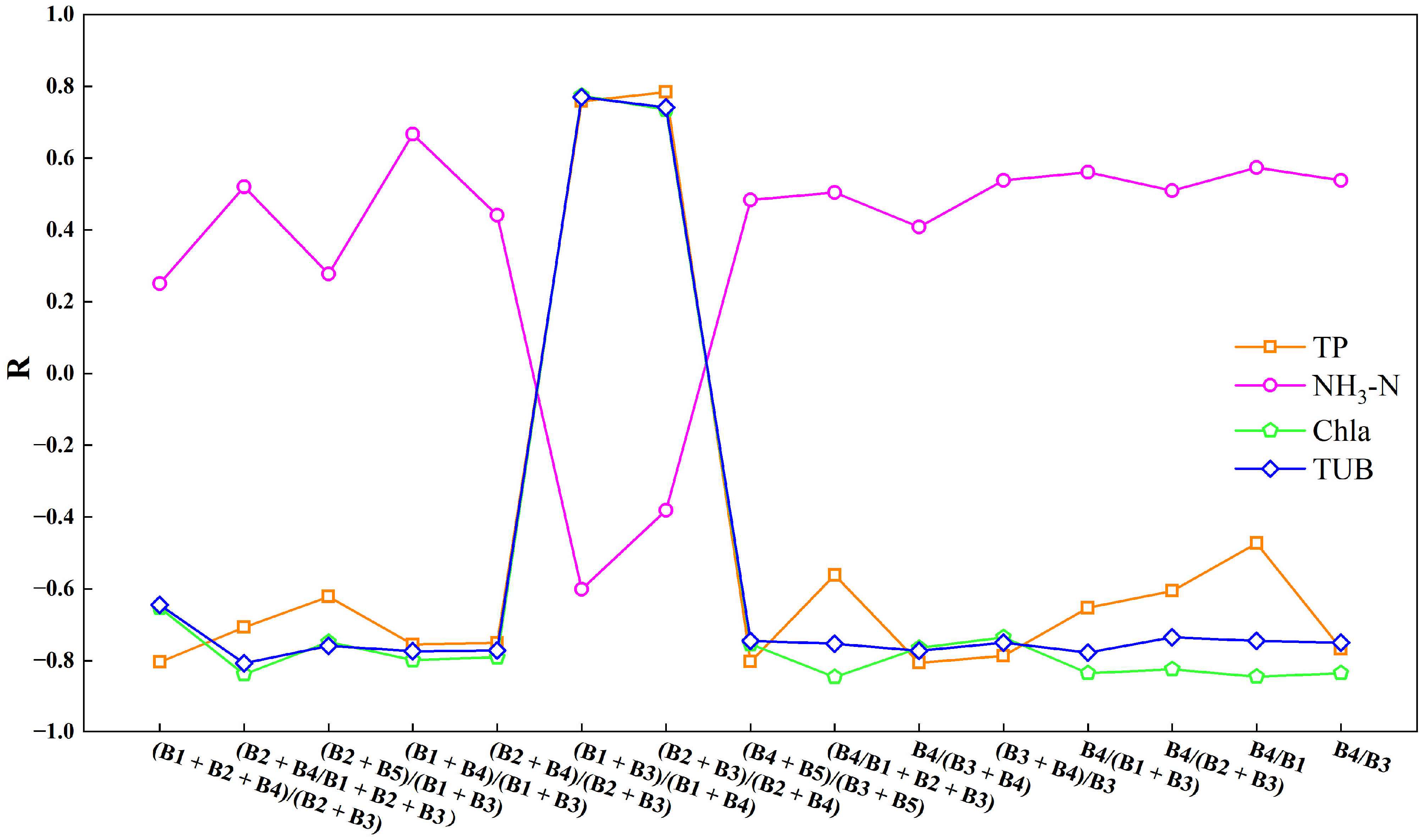
The reflectance values of five bands of each sampling point are obtained from the multispectral images of the UAV, and the variation rules between the reflectance values and the concentration of water quality parameters are analyzed (Figure 4). Strong absorption peaks are observed in the blue and red bands, while reflection peaks are found in the green and infrared bands. The reflectance curves near the green, red, and near-red bands show large variations. Reflectance values from each band are combined, followed by Pearson correlation analysis with water quality parameter concentrations (Figure 5). The combination of bands with the highest correlation is identified and used as input to the model to enhance its predictive performance [57]. The model’s input variables are determined by selecting the five spectral bands with the highest correlation for each water quality parameter (Table 3).
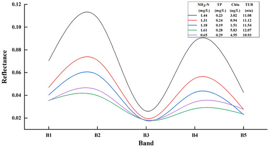
Figure 4.
Spectral feature analysis.
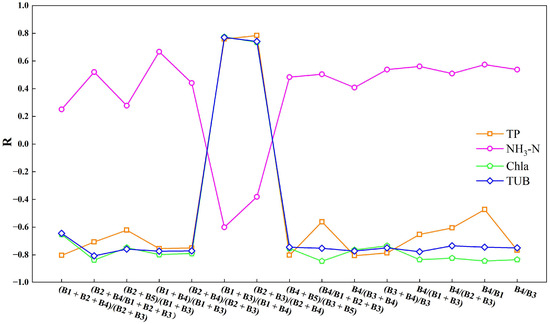
Figure 5.
The combination of the 15 bands with the highest correlation.
Table 3.
The five most correlated band combinations were input into the model as feature selection.
3.3. Predictive Performances
Seven intelligent optimization algorithms were used to optimize the established SVR model. The independent variable of the model was a combination of bands with high correlation after feature selection, and the dependent variables were the concentrations of Chla, TP, NH3-N, and TUB. The predicted values were visualized and compared with the measured values through scatter plots to assess the fitting ability of the model. The optimized SVR model’s accuracy could be more effectively gauged by analyzing the errors between the predicted and measured values.
3.3.1. Chlorophyll (Chla)
Compared with the unoptimized SVR model (Figure 6), the R2 values of the SVR model optimized by both GWO and GA algorithms exceed 0.910, while the SVR model is only 0.762. Various optimization algorithms have enhanced the performance of the SVR model, with the GWO-SVR model exhibiting superior performance in Chla prediction. Compared with the SVR models, the R2 values of SVR models optimized by GWO, GA, PSO, ACO, FA, SSA, and HPO improved by 20.08%, 19.82%, 14.30%, 5.64%, 8.14%, 5.64%, and 11.02%, respectively. Meanwhile, the reductions in RMSE values were 23.34%, 16.94%, 15.42%, 11.11%, 14.79%, 11.00%, and 24.90%, respectively. The reductions in MAE values were 46.61%, 30.67%, 27.72%, 17.70%, 22.71%, 17.70%, and 47.78%, respectively.
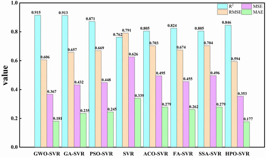
Figure 6.
Comparison of the accuracy of basic-SVR and optimized-SVR models for Chla.
Comparing the GWO algorithm with other optimization algorithms (GA, PSO, ACO, FA, SSA, and HPO) led to improvements in R2 by 0.22%, 5.05%, 13.67%, 11.04%, 13.67%, and 8.16%. Simultaneously, RMSE witnessed reductions of 7.76%, 9.42%, 13.80%, 10.09%, 13.92%, and −0.02%, while MAE decreased by 22.98%, 26.12%, 35.13%, 30.92%, 35.13%, and −2.26%.
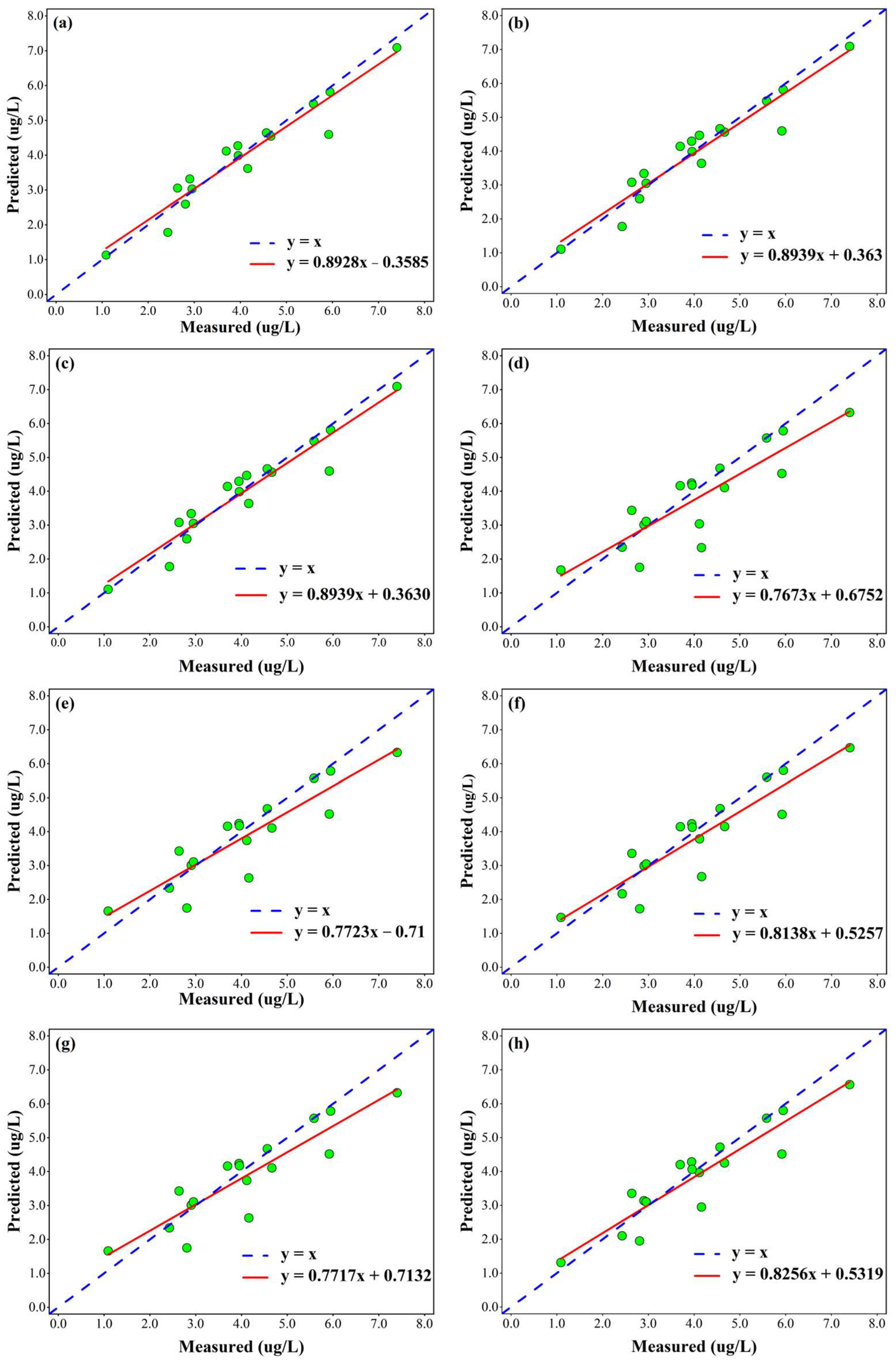
According to the fit plots of predicted and true values, it is evident that the optimized SVR model shows excellent model fit in Chla prediction (Figure 7). The predicted and measured values are uniformly distributed around a 1:1 straight line, indicating that the optimized SVR model shows good fitting ability for Chla. These results suggest that the SVR model optimized with the GA algorithm and GWO algorithm performs well in terms of Chla prediction capability.
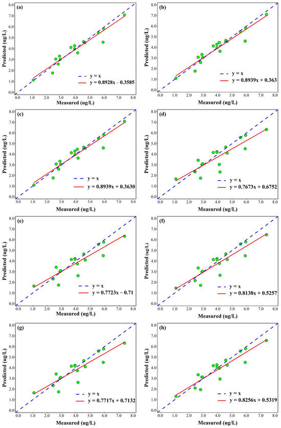
Figure 7.
The scatter plots of predicted values and measured values of Chla using different SVR models. (a) GWO-SVR; (b) GA-SVR; (c) PSO-SVR; (d) SVR; (e) ACO-SVR; (f) FA-SVR; (g) SSA-SVR; (h) HPO-SVR.
3.3.2. Total Phosphorus (TP)
For TP prediction, the SVR models optimized by the GWO and GA algorithms perform well, with their R2 values greater than 0.820 (Figures S1 and S2). In particular, the GWO-SVR model shows the best results in terms of fitting the measured data (R2 = 0.827, RMSE = 0.068, MSE = 0.005, MAE = 0.005). In contrast, the prediction performance of the unoptimized SVR model is the worst (R2 = 0.621, RMSE = 0.102, MSE = 0.010, MAE = 0.010). In general, its fitting ability is decreased when compared to that of the Chla (R2 = 0.762).
For GWO algorithm, when compared with GA, PSO, ACO, FA, SSA, and HPO, R2 increases by 0.00%, 2.87%, 2.35%, 2.99%, 2.61%, and 2.61%. Correspondingly, RMSE witnessed reductions of −1.49%, 5.56%, 4.23%, 5.56%, 4.23%, and 4.23%, while MAE decreased by 0.00%, 28.57%, 28.57%, 28.57%, 28.57%, and 28.57%.
3.3.3. Ammonia Nitrogen (NH3-N)
From the performance and prediction results of the model for predicting NH3-N concentration (Figures S3 and S4), notably, the SVR models, subjected to refinement via the GWO, PSO, and HPO optimization algorithms, have exhibited commendable performance, each boasting an R2 value surpassing 0.83. The SVR model optimized by GA and SSA algorithms also showed a strong fitting ability, and, overall, the PSO-SVR model has the best performance in the prediction of Chla (R2 = 0.846, RMSE = 0.171, MSE = 0.029, and MAE = 0.136), followed by the GWO-SVR model (R2 = 0.838, RMSE = 0.145, MSE = 0.021 and MAE = 0.111). However, compared with the predictive performance of TP and Chla, the performance of the SVR model for NH3-N prediction still needed further improvement.
In the comparison of the GWO algorithm with other optimization algorithms (GA, PSO, ACO, FA, SSA, and HPO), R2 advanced by 8.11%, 7.24%, 8.11%, 6.95%, 7.53%, and 0.76%. Concurrently, RMSE witnessed reductions of 5.07%, 1.29%, 16.07%, 8.79%, 9.75%, and 0.39%, while MAE decreased by 13.75%, 8.73%, 36.81%, 21.59%, 27.06%, and 1.99%.
3.3.4. Turbidity (TUB)
The prediction performances of the SVR model optimized by the GWO and HPO algorithms for TUB are the most outstanding, with R2 > 0.790 (Figure S5). The SVR model optimized by the other five optimization algorithms also depicts a strong fitting ability (Figure S6). The GWO-SVR algorithm performs the best in the prediction performance of the TUB-measured data (R2 = 0.809, RMSE = 0.809, MSE = 0.655, and MAE = 0.400). Meanwhile, the R2 of the basic SVR algorithm is only 0.620, which is inferior to the optimization algorithms.
When the GWO algorithm was compared with other optimization algorithms (GA, PSO, ACO, FA, SSA, and HPO), its R2 exhibited improvements by 4.10%, −0.95%, 6.75%, 9.83%, 4.62%, and 0.60%. Simultaneously, RMSE witnessed reductions of 15.20%, 15.20%, 42.00%, 41.53%, 44.44%, and 16.67%, while MAE decreased by 18.38%, 18.38%, 43.37%, 40.96%, 43.37%, and 28.39%.
3.3.5. Comparison of the Performances of Eight SVR Models
The results of this study show that the GA-SVR and GWO-SVR models perform optimally in the prediction of Chla, with improvements in R2 values of 19.81% and 20.08%, reductions in RMSE values of 16.94% and 23.39%, and MAE values reduced by 30.68% and 46.61%, respectively, compared to the basic-SVR model. In terms of the prediction performance of TP, the SVR model optimized by the GA algorithm and the GWO algorithm also performs well, with the R2 values improved by 33.17% and 33.17%, the RMSE values reduced by 33.34% and 33.33%, and the MAE values reduced by 47.80% and 47.80%, respectively. For the prediction of NH3-N, the SVR model optimized by PSO and GWO algorithms also performs well, with their R2 values improved by 24.5% and 24.3%, the RMSE values reduced by 41.43% and 50.34%, and the MAE values reduced by 56.92% and 47.02%, respectively. For TUB prediction, the SVR models optimized by the HPO algorithm and the GWO algorithm also perform well, with increases in R2 values of 28.47% and 29.45%, decreases in RMSE values of 36.30% and 36.83%, and the MAE values reduced by 45.08% and 44.08%, respectively. In summary, the optimized SVR model significantly improves the accuracy of the SVR model. This could be because, when building the model, its core function and penalty settings need manual adjustments. Different datasets might require different parameter setups and it is challenging to manually find the best parameters. This is consistent with previous research.
The prediction performance of eight models is compared and it is found that GA-SVR performed the best in TP (R2 = 0.827). However, the prediction performances of TUB (R2 = 0.740) and NH3-N (R2 = 0.805) are relatively poor, ranking fourth and fifth among eight models. Such results indicated that GA-SVR has certain instability in the prediction of water quality indicators in the Yudai River. The differences in performance may be because the GA is sensitive to its settings, needing manual adjustments. GA mimics genetic processes, which have randomness, leading to unpredictable results. Moreover, GA tends to require a lot of training data to work well on complex problems [58]. The PSO-SVR model demonstrated excellent predictive performance regarding NH3-N (R2 = 0.846), yet it fell short in predicting other water quality parameters; perhaps it has fallen into a local optimum when predicting NH3-N [59]. While the GWO-SVR model does not exhibit the best predictive performance for TP (R2 = 0.827) and NH3-N (R2 = 0.838) among the eight models, it consistently ranked second in eight models. Moreover, it showcased the best predictive performance for Chla (R2 = 0.915) and TUB (R2 = 0.800), highlighting its stability in predicting water quality concentrations for small-scale rivers. Thus, considering all aspects, the GWO-SVR model demonstrated the most excellent performance among the eight models.
3.4. Stability Analysis of GWO-SVR Model
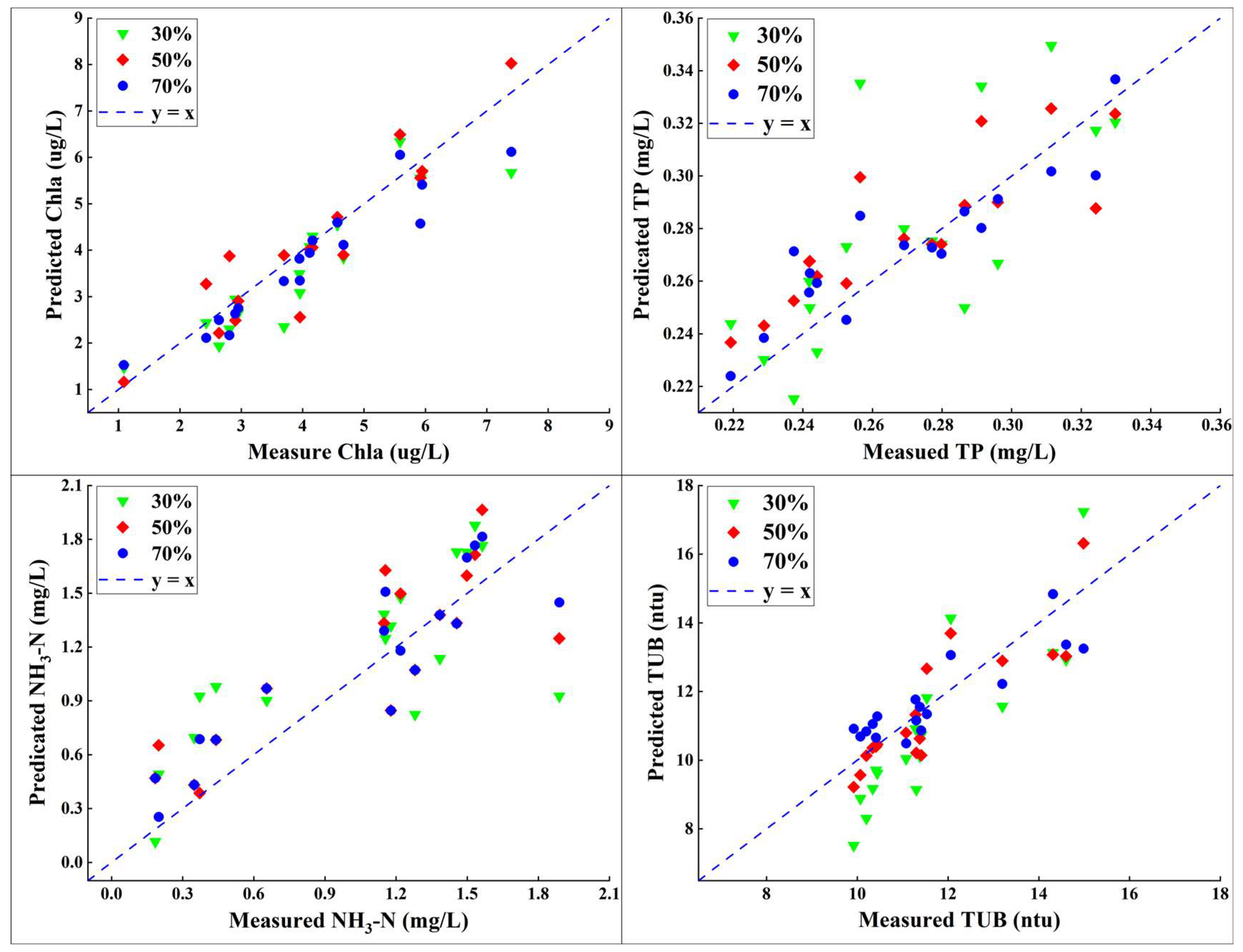
To further explore the stability of the GWO-SVR model under fewer samples in this study, 30% (n = 20), 50% (n = 34), and 70% (n = 47) of the total number of samples (n = 67) are randomly selected as new training samples, there is no alteration in the test data. By analyzing the prediction results of the model on the test set under training with fewer samples, the stability of the model is evaluated.
The experimental results show that the prediction of TP and NH3-N are influenced by the number of samples, and the prediction accuracy of the model has improved as the number of samples increases (Figure 8 and Table 4). In contrast, the prediction results of Chla and TUB are affected by the sample size less and their prediction accuracies are relatively high and stable. Such difference may be because both Chla and TUB are optically sensitive parameters, there is a clear correlation with the spectral responses in the water body, and this correlation is more accurate to capture [60]. However, non-optically sensitive parameters, e.g., TP and NH3-H, may be affected by hydrodynamic changes in water, temperature, pH, etc. Consequently, the retrieval of TP and NH3-N of the SVR model only shows a certain degree of instability, especially under the constraint of a limited sample size [61,62].
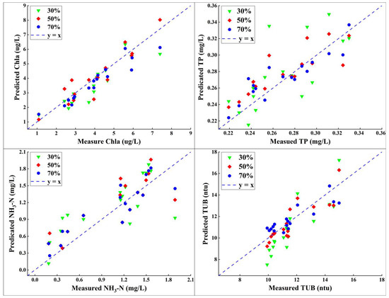
Figure 8.
Scatter plots of different data volumes.
Table 4.
Model accuracy of different data volumes.
3.5. Applicability of GWO-SVR Model
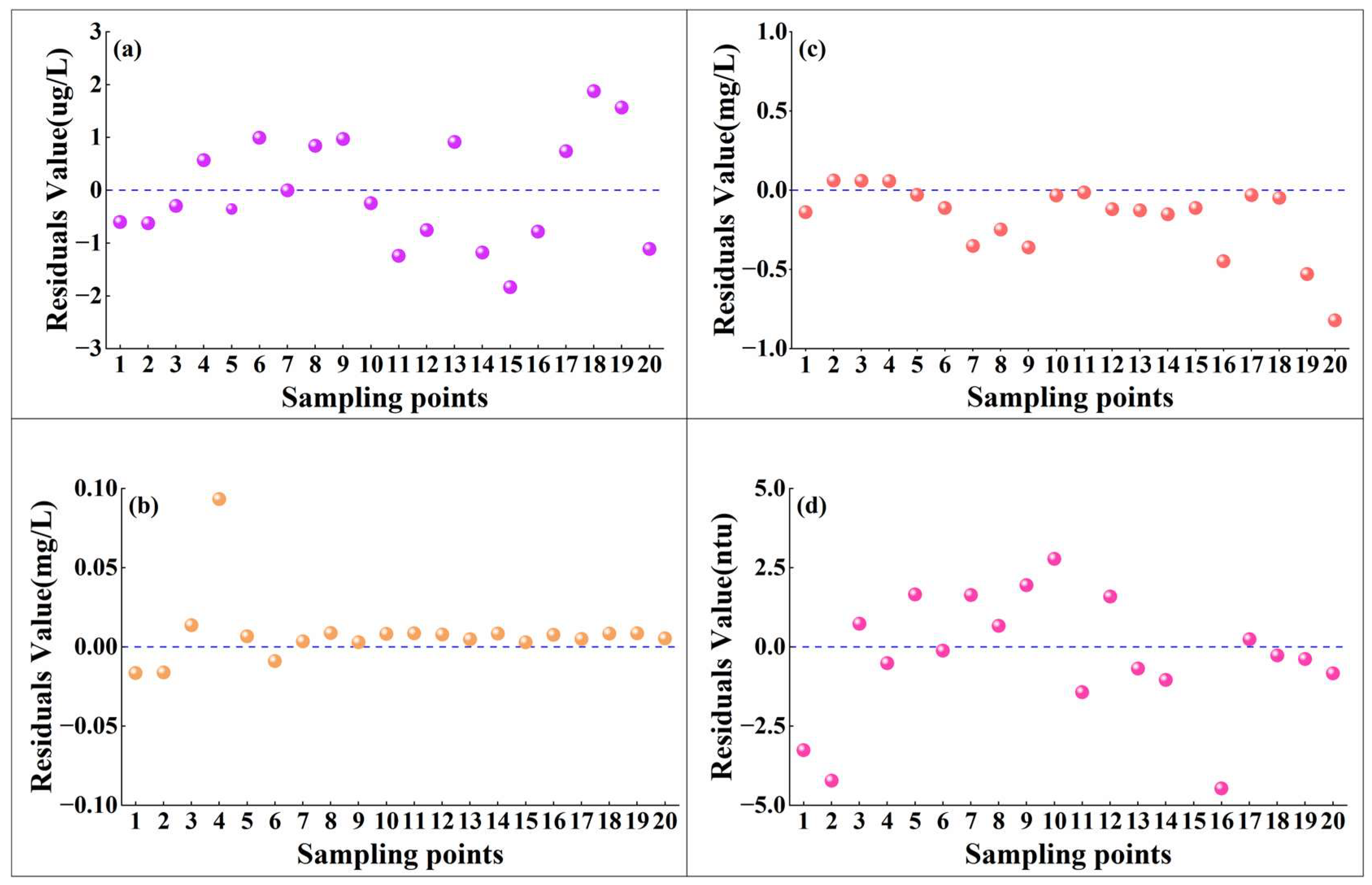
To validate the applicability of the GWO-SVR model to the same watershed at different times, new data are introduced. The UAV images of the Yudai River captured on 1 September 2022 are inputted into the constructed model to obtain the corresponding predicted values, and then they are compared to the corresponding measured values (Figure 9).

Figure 9.
Residual plots of measured and predicted values. (a) Chla; (b) TP; (c) NH3-N; (d) TUB.
In general, a consistent correspondence between the predicted Chla, TP, NH3-N, and TUB values via GWO-SVR models and their measured values is observed. Although minor discrepancies were recorded at several specific points, the applicability of the model is not significantly undermined. Consequently, the established GWO-SVR model demonstrates strong applicability for water quality inversion across various time intervals.
3.6. Inversion Results of the Lower Reaches of the Yudai River Based on the GWO-SVR
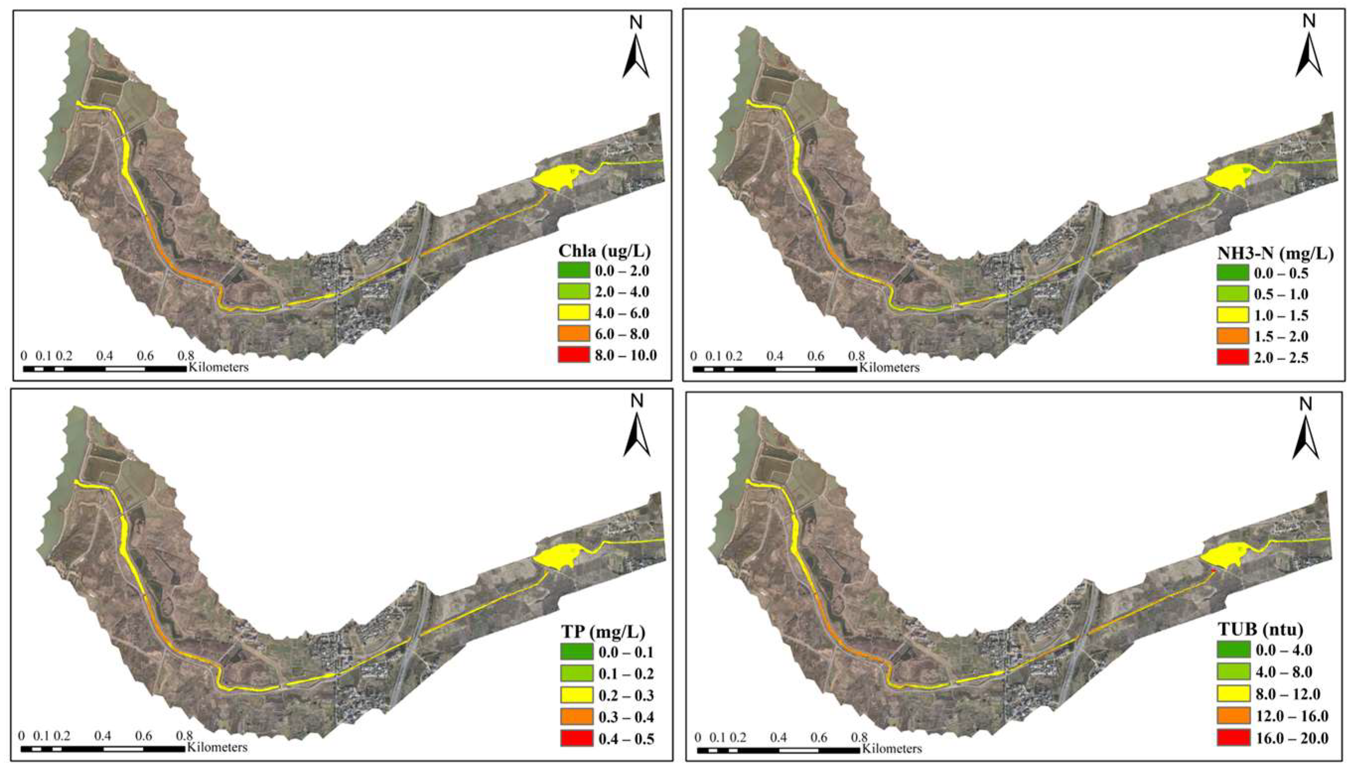
The established GWO-SVR model is applied for the inversion of Chla, TUB, TP, and NH3-N concentrations in the Yudai River (Figure 10). According to the results, the levels of Chla, TP, NH3-N, and TUB ranged from 0.980 to 7.726 ug/L, 0.219 to 0.351 mg/L, 0.185 to 2.057 mg/L, and 8.689 to 14.987 ntu, respectively. The inversion results are well consistent with the measured values, indicating the validity of the inversion models.
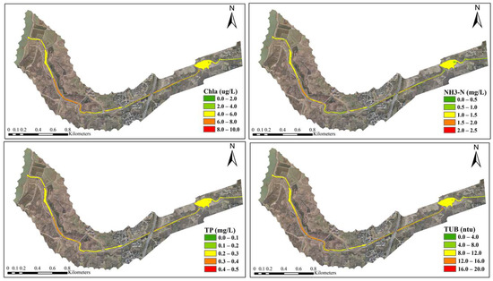
Figure 10.
Results of water quality inversion in the study area.
It is found that some water areas are overgrown with weeds near the shore and trees are standing around, and these factors may influence the spectral characteristics of the water bodies during the inversion and cause deviations. However, such deviations are still within the acceptable range and do not significantly affect the quality of the inversion of the selected river section.
4. Discuss
4.1. Potential Pollution Source Analysis
The downstream of the Yudai River is selected as the study area and it is divided into five sub-areas, i.e., Region A, B, C, D, and E (Figure 11). The inversion results reveal that the concentrations of TP, Chla, NH3-N, and TUB are relatively higher in Regions B, D, and E. Regions A and C are in a medium to low concentration. Such a phenomenon may be due to the following reasons: (1) the existence of agricultural cultivation areas around Region B may result in the massive loss of nitrogen and phosphorus from soil and entering into the water body via runoff and (2) Region D, as a typical residential area, where the untreated domestic wastewater, domestic garbage, and animal manure washed into the river during rainfall events, thus resulting in increased concentrations of nitrogen and phosphorus elements. These elements also accelerated the growth of algae and contributed to the higher Chla concentrations in the water body. In Region E, the high concentrations of NH3-N, TP, and TUB could be attributed to the previous presence of free-range livestock. Runoffs from livestock and feed residues are entered into the water body, as well as domestic wastewater from the neighboring residential areas that flow into the river. In addition, the narrow channel and slow flow of the river are preferential for the growth of algae, and thus high concentrations of Chla are observed.
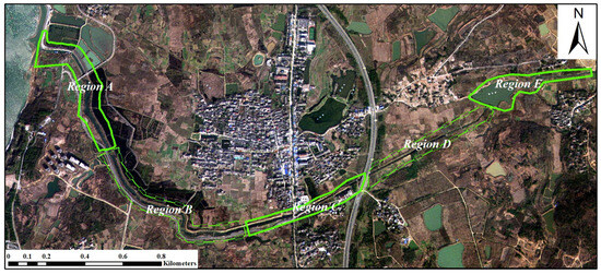
Figure 11.
Detailed regional division satellite images of the study area.
The levels of water quality parameters in Region A were maintained at moderate levels. This might be because Region A is an inlet to the Chaohu Lake with a wide watercourse and strong liquidity and the water body has relatively higher self-purification capacity [63]. However, during the long-term monitoring, the water quality remained in the range of Class IV water standards (China Environmental Quality Standard for surface water. GB 3838-2002 [64]), indicating the relatively serious pollution status of this river. This indicated to some extent that untreated domestic sewage, livestock breeding effluent, and nitrogen and phosphorus loss from agricultural processes are the main sources of pollution in the lower Yudai River.
4.2. Compare with Other Studies
In comparison with previous research results (Table 5), the water quality parameter inversion based on UAV multispectral images in this study showed an R2 value of 0.8–0.915 range, while the water quality parameter inversion based on satellite data on oceans and lakes showed a lower fitness (R2 in the range of 0.69–0.83). For example, Kim et al. [65] employed Sentinel-2 data and machine learning algorithms to assess chlorophyll-a (Chla) in coastal areas. The best-performing model achieved an R2 of 0.75. Wu et al. predicted the chlorophyll-A concentration in the Ulansu Sea using the GA-SVR model and its R2 = 0.87 [66]. Ren et al. employed a GWO-SVR model in conjunction with Sentinel-2 satellite data to predict chlorophyll-a in Tangdao Bay, achieving an R2 of 0.71 [67]. During the acquisition of spectral data, satellite remote sensing is susceptible to atmospheric scattering and surface light from the water body, and these influences cannot be eliminated [68]. In contrast, UAV remote sensing can eliminate atmospheric interference and efficiently capture water spectral parameters. To sum up, water quality inversion based on UAV remote sensing achieves higher accuracy [69,70]. Meanwhile, compared with other widely used machine learning models, for instance, Chen et al. used the GA-XGBoost model to invert water quality parameters of small and medium-sized rivers, and the R2 values of their models were in the range of 0.597 to 0.855 [71]. Leong et al. predicted water quality based on Least Square-Support Vector Machine (LS-SVM), achieving an R2 of 0.92 [72]. Zhang et al., through a comparative analysis of several SVR models for predicting dissolved oxygen, found that GS-SVR and GA-SVR exhibited the best performance, with R2 values reaching 0.81 and 0.84, respectively [73]. In Section 3.4 and Section 3.5, the stability of the GWO-SVR model has been confirmed under limited samples, demonstrating excellent adaptability across different periods. Such results suggested that the GWO-SVR model has an excellent performance in the estimation of water quality parameters in small-sized rivers.
Table 5.
Comparison with previous research results.
4.3. Limitations and Future Perspectives
In this study, the application of unmanned aerial vehicle (UAV) multispectral data and the Grey Wolf Optimizer-Support Vector Regression (GWO-SVR) model in the water quality monitoring of small-micro water bodies, particularly for parameters such as chlorophyll-a (Chla), total phosphorus (TP), ammonia nitrogen (NH3-N), and turbidity (Turb), has shown promising results. However, further exploration is needed to assess the applicability of GWO-SVR in different types of water bodies and for estimating various water quality indicators. Additionally, due to the relatively small sample size in this study and the limitation of having water quality data for only one season, understanding the temporal variations in river water quality necessitates further investigation. Future work will focus on expanding the database by integrating water quality data from multiple seasons to achieve a more comprehensive understanding of the dynamic changes in water quality [74]. This provides significant inspiration for our research and we plan to apply this approach in our study area, aiming to establish a comprehensive monitoring system integrating aerial and ground observations [75].
5. Conclusions
In conclusion, based on the multispectral UAV images and ground monitoring data, the SVR model optimized by seven intelligent algorithms and the initial SVR model were constructed to predict the water quality parameters (Chla, TP, NH3-N, and TUB) of small-micro rivers, and their prediction effects were compared. The experimental results show that the GWO-SVR model has the most significant prediction effect on the four water quality indicators of Yudai River, and its R2 values are all greater than 0.80. Meanwhile, by reducing the sample size of the training set and validating the dataset directly for different periods, the GWO-SVR model still exhibits significant stability and applicability. The results show that the GWO-SVR model has a high prediction accuracy for the water quality of small rivers, which can provide a scientific basis for the monitoring and prevention of small-micro water pollution.
Supplementary Materials
The following are available online at https://www.mdpi.com/article/10.3390/su16020559/s1. Supporting Information includes Table S1 and Figures S1–S6, as noted in the texts.
Author Contributions
K.Y.: Conceptualization; Data curation; Formal analysis; Investigation; Methodology; Software; Validation; Visualization; Writing—original draft; Writing—review and editing. Y.C.: Data curation; Formal analysis; Investigation; Methodology; Software. Y.L.: Funding acquisition; Project administration. X.Z. Methodology; Writing—review and editing; Funding acquisition; Project administration. B.Z. and Z.G.: Investigation; Data curation. F.L.: Writing—review and editing; Formal analysis. Y.H.: Methodology; Writing—review and editing. All authors have read and agreed to the published version of the manuscript.
Funding
This research was financially supported by the National Natural Science Foundation of China (42377408), University Natural Science Research Project of Anhui Province (No. KJ2021A0081), Open Project of the State Environmental Protection Key Laboratory of Soil Environmental Management and Pollution Control (No. SEMPC 2023003), and Feidong County Agricultural Non-Point Source Pollution Control Pilot Work Third Party Service Project (2023ADDFZ00164).
Institutional Review Board Statement
Not applicable.
Informed Consent Statement
Not applicable.
Data Availability Statement
The data are not publicly available due to privacy.
Conflicts of Interest
The authors declare no conflict of interest.
References
- Feng, S.; Liu, S.; Huang, Z.; Jing, L.; Zhao, M.; Peng, X.; Yan, W.; Wu, Y.; Lv, Y.; Smith, A.R.; et al. Inland Water Bodies in China: Features Discovered in the Long-Term Satellite Data. Proc. Natl. Acad. Sci. USA 2019, 116, 25491–25496. [Google Scholar] [CrossRef] [PubMed]
- Abowei, J. Salinity, Dissolved Oxygen, pH and Surface Water Temperature Conditions in Nkoro River, Niger Delta, Nigeria. Adv. J. Food Ence Technol. 2010, 2, 36–40. [Google Scholar]
- Liu, M.; Liu, Z.; Jiang, T.; Chen, X.; Yu, H. Institutional Reform of Water Resources Management in China. In Hydrological Sciences for Managing Water Resources in the Asian Developing World; International Association of Hydrological Sciences: Wallingford, UK, 2008; pp. 319–325. [Google Scholar]
- Mentzafou, A.; Panagopoulos, Y.; Dimitriou, E. Designing the National Network for Automatic Monitoring of Water Quality Parameters in Greece. Water 2019, 11, 1310. [Google Scholar] [CrossRef]
- Jay, S.; Guillaume, M.; Minghelli, A.; Deville, Y.; Chami, M.; Lafrance, B.; Serfaty, V. Hyperspectral Remote Sensing of Shallow Waters: Considering Environmental Noise and Bottom Intra-Class Variability for Modeling and Inversion of Water Reflectance. Remote Sens. Environ. 2017, 200, 352–367. [Google Scholar] [CrossRef]
- He, Y.; Gong, Z.; Zheng, Y.; Zhang, Y. Inland Reservoir Water Quality Inversion and Eutrophication Evaluation Using BP Neural Network and Remote Sensing Imagery: A Case Study of Dashahe Reservoir. Water 2021, 13, 2844. [Google Scholar] [CrossRef]
- García-Nieto, P.J.; García-Gonzalo, E.; Fernández, J.A.; Muñiz, C.D. Using Evolutionary Multivariate Adaptive Regression Splines Approach to Evaluate the Eutrophication in the Pozón de La Dolores Lake (Northern Spain). Ecol. Eng. 2016, 94, 136–151. [Google Scholar] [CrossRef]
- Arabi, B.; Salama, M.S.; Pitarch, J.; Verhoef, W. Integration of In-Situ and Multi-Sensor Satellite Observations for Long-Term Water Quality Monitoring in Coastal Areas. Remote Sens. Environ. 2020, 239, 111632. [Google Scholar] [CrossRef]
- Pahlevan, N.; Sarkar, S.; Franz, B.A.; Balasubramanian, S.V.; He, J. Sentinel-2 MultiSpectral Instrument (MSI) Data Processing for Aquatic Science Applications: Demonstrations and Validations. Remote Sens. Environ. 2017, 201, 47–56. [Google Scholar] [CrossRef]
- Kloiber, S.M.; Brezonik, P.L.; Bauer, M.E. Application of Landsat Imagery to Regional-Scale Assessments of Lake Clarity. Water Res. 2002, 36, 4330–4340. [Google Scholar] [CrossRef]
- Mertes, L.A.K.; Smith, M.O.; Adams, J.B. Estimating Suspended Sediment Concentrations in Surface Waters of the Amazon River Wetlands from Landsat Images. Remote Sens. Environ. 1993, 43, 281–301. [Google Scholar] [CrossRef]
- Sòria-Perpinyà, X.; Vicente, E.; Urrego, P.; Pereira-Sandoval, M.; Ruíz-Verdú, A.; Delegido, J.; Soria, J.M.; Moreno, J. Remote Sensing of Cyanobacterial Blooms in a Hypertrophic Lagoon (Albufera of València, Eastern Iberian Peninsula) Using Multitemporal Sentinel-2 Images. Sci. Total Environ. 2020, 698, 134305. [Google Scholar] [CrossRef] [PubMed]
- Xu, J.; Gao, C.; Wang, Y. Extraction of Spatial and Temporal Patterns of Concentrations of Chlorophyll-a and Total Suspended Matter in Poyang Lake Using GF-1 Satellite Data. Remote Sens. 2020, 12, 622. [Google Scholar] [CrossRef]
- Cillero Castro, C.; Domínguez Gómez, J.A.; Delgado Martín, J.; Hinojo Sánchez, B.A.; Cereijo Arango, J.L.; Cheda Tuya, F.A.; Díaz-Varela, R. An UAV and Satellite Multispectral Data Approach to Monitor Water Quality in Small Reservoirs. Remote Sens. 2020, 12, 1514. [Google Scholar] [CrossRef]
- Cheng, K.H.; Chan, S.N.; Lee, J.H.W. Remote Sensing of Coastal Algal Blooms Using Unmanned Aerial Vehicles (UAVs). Mar. Pollut. Bull. 2020, 152, 110889. [Google Scholar] [CrossRef] [PubMed]
- Bie, W.; Fei, T.; Liu, X.; Liu, H.; Wu, G. Small Water Bodies Mapped from Sentinel-2 MSI (MultiSpectral Imager) Imagery with Higher Accuracy. Int. J. Remote Sens. 2020, 41, 7912–7930. [Google Scholar] [CrossRef]
- Riley, W.D.; Potter, E.C.E.; Biggs, J.; Collins, A.L.; Jarvie, H.P.; Jones, J.I.; Kelly-Quinn, M.; Ormerod, S.J.; Sear, D.A.; Wilby, R.L.; et al. Small Water Bodies in Great Britain and Ireland: Ecosystem Function, Human-Generated Degradation, and Options for Restorative Action. Sci. Total Environ. 2018, 645, 1598–1616. [Google Scholar] [CrossRef]
- Matsushita, B.; Yang, W.; Chang, P.; Yang, F.; Fukushima, T. A Simple Method for Distinguishing Global Case-1 and Case-2 Waters Using SeaWiFS Measurements. ISPRS J. Photogramm. Remote Sens. 2012, 69, 74–87. [Google Scholar] [CrossRef]
- Yu, X.; Yi, H.; Liu, X.; Wang, Y.; Liu, X.; Zhang, H. Remote-Sensing Estimation of Dissolved Inorganic Nitrogen Concentration in the Bohai Sea Using Band Combinations Derived from MODIS Data. Int. J. Remote Sens. 2016, 37, 327–340. [Google Scholar] [CrossRef]
- Zhou, Y.; He, B.; Fu, C.; Xiao, F.; Feng, Q.; Liu, H.; Zhou, X.; Yang, X.; Du, Y. An Improved Forel–Ule Index Method for Trophic State Assessments of Inland Waters Using Landsat 8 and Sentinel Archives. GISci. Remote Sens. 2021, 58, 1316–1334. [Google Scholar] [CrossRef]
- Zhang, J.M.; Harman, M.; Ma, L.; Liu, Y. Machine Learning Testing: Survey, Landscapes and Horizons. IEEE Trans. Softw. Eng. 2022, 48, 1–36. [Google Scholar] [CrossRef]
- Bourel, M.; Segura, A.M.; Crisci, C.; López, G.; Sampognaro, L.; Vidal, V.; Kruk, C.; Piccini, C.; Perera, G. Machine Learning Methods for Imbalanced Data Set for Prediction of Faecal Contamination in Beach Waters. Water Res. 2021, 202, 117450. [Google Scholar] [CrossRef] [PubMed]
- Hafeez, S.; Wong, M.S.; Ho, H.C.; Nazeer, M.; Nichol, J.; Abbas, S.; Tang, D.; Lee, K.H.; Pun, L. Comparison of Machine Learning Algorithms for Retrieval of Water Quality Indicators in Case-II Waters: A Case Study of Hong Kong. Remote Sens. 2019, 11, 617. [Google Scholar] [CrossRef]
- Wu, B.; Yang, J.; Chen, J.; Chen, J.; Wu, J. A Method of Obtaining Accurate Active Area of Remote Sensing Image and Application in Mosaicking. In Proceedings of the 2nd International Conference on Remote Sensing, Environment and Transportation Engineering, Nanjing, China, 1–3 June 2012; pp. 1–4. [Google Scholar]
- Sedaghat, A.; Mokhtarzade, M.; Ebadi, H. Uniform Robust Scale-Invariant Feature Matching for Optical Remote Sensing Images. IEEE Trans. Geosci. Remote Sens. 2011, 49, 4516–4527. [Google Scholar] [CrossRef]
- Rahmati, O.; Darabi, H.; Panahi, M.; Kalantari, Z.; Naghibi, S.A.; Ferreira, C.S.S.; Kornejady, A.; Karimidastenaei, Z.; Mohammadi, F.; Stefanidis, S.; et al. Development of Novel Hybridized Models for Urban Flood Susceptibility Mapping. Sci. Rep. 2020, 10, 12937. [Google Scholar] [CrossRef]
- Zhan, A.; Du, F.; Chen, Z.; Yin, G.; Wang, M.; Zhang, Y. A Traffic Flow Forecasting Method Based on the GA-SVR. J. High Speed Netw. 2022, 28, 97–106. [Google Scholar] [CrossRef]
- Li, Y.; He, L.; Peng, B.; Fan, K.; Tong, L. Remote Sensing Inversion of Water Quality Parameters in Longquan Lake Based on PSO-SVR Algorithm. In Proceedings of the IGARSS 2018–2018 IEEE International Geoscience and Remote Sensing Symposium, IEEE, Valencia, Spain, 22–27 July 2018; pp. 9268–9271. [Google Scholar]
- Eslamitabar, V.; Ahmadi, F.; Sharafati, A.; Rezaverdinejad, V. Bivariate Simulation of River Flow Using Hybrid Intelligent Models in Sub-Basins of Lake Urmia, Iran. Acta Geophys. 2023, 71, 873–892. [Google Scholar] [CrossRef]
- Mahdavi-Meymand, A.; Sulisz, W.; Zounemat-Kermani, M. A Comprehensive Study on the Application of Firefly Algorithm in Prediction of Energy Dissipation on Block Ramps. Eksploat. Niezawodn. 2022, 24, 200–210. [Google Scholar] [CrossRef]
- Su, X.; He, X.; Zhang, G.; Chen, Y.; Li, K. Research on SVR Water Quality Prediction Model Based on Improved Sparrow Search Algorithm. Comput. Intell. Neurosci. 2022, 2022, e7327072. [Google Scholar] [CrossRef]
- Fu, M.; Liu, Q. An Improved Hunter-Prey Optimization Algorithm and Its Application. In Proceedings of the 2022 IEEE International Conference on Networking, Sensing and Control (ICNSC), Shanghai, China, 15–18 December 2022; pp. 1–7. [Google Scholar]
- Yang, H.; Kong, J.; Hu, H.; Du, Y.; Gao, M.; Chen, F. A Review of Remote Sensing for Water Quality Retrieval: Progress and Challenges. Remote Sens. 2022, 14, 1770. [Google Scholar] [CrossRef]
- HJ 494—2009; Water Quality-Guidance on Sampling Techniques. Ministry of Ecology and Environment of the People’s Republic of China: Beijing, China, 2009.
- Dinguirard, M.; Slater, P.N. Calibration of Space-Multispectral Imaging Sensors: A Review. Remote Sens. Environ. 1999, 68, 194–205. [Google Scholar] [CrossRef]
- Schramm, S.; Rangel, J.; Salazar, D.A.; Schmoll, R.; Kroll, A. Target Analysis for the Multispectral Geometric Calibration of Cameras in Visual and Infrared Spectral Range. IEEE Sens. J. 2021, 21, 2159–2168. [Google Scholar] [CrossRef]
- Cao, S.; Danielson, B.; Clare, S.; Koenig, S.; Campos-Vargas, C.; Sanchez-Azofeifa, A. Radiometric Calibration Assessments for UAS-Borne Multispectral Cameras: Laboratory and Field Protocols. ISPRS J. Photogramm. Remote Sens. 2019, 149, 132–145. [Google Scholar] [CrossRef]
- Montesinos López, O.A.; Montesinos López, A.; Crossa, J. Support Vector Machines and Support Vector Regression. In Multivariate Statistical Machine Learning Methods for Genomic Prediction; Montesinos López, O.A., Montesinos López, A., Crossa, J., Eds.; Springer International Publishing: Cham, Switzerland, 2022; pp. 337–378. ISBN 978-3-030-89010-0. [Google Scholar]
- Leng, T.; Li, F.; Chen, Y.; Tang, L.; Xie, J.; Yu, Q. Fast Quantification of Total Volatile Basic Nitrogen (TVB-N) Content in Beef and Pork by near-Infrared Spectroscopy: Comparison of SVR and PLS Model. Meat Sci. 2021, 180, 108559. [Google Scholar] [CrossRef] [PubMed]
- Were, K.; Bui, D.T.; Dick, Ø.B.; Singh, B.R. A Comparative Assessment of Support Vector Regression, Artificial Neural Networks, and Random Forests for Predicting and Mapping Soil Organic Carbon Stocks across an Afromontane Landscape. Ecol. Indic. 2015, 52, 394–403. [Google Scholar] [CrossRef]
- de Cos Juez, F.J.; García Nieto, P.J.; Martínez Torres, J.; Taboada Castro, J. Analysis of Lead Times of Metallic Components in the Aerospace Industry through a Supported Vector Machine Model. Math. Comput. Model. 2010, 52, 1177–1184. [Google Scholar] [CrossRef]
- Mirjalili, S.; Mirjalili, S.M.; Lewis, A. Grey Wolf Optimizer. Adv. Eng. Softw. 2014, 69, 46–61. [Google Scholar] [CrossRef]
- Frenzel, J.F. Genetic Algorithms. IEEE Potentials 1993, 12, 21–24. [Google Scholar] [CrossRef]
- Lambora, A.; Gupta, K.; Chopra, K. Genetic Algorithm–A Literature Review. In Proceedings of the 2019 International Conference on Machine Learning, Big Data, Cloud and Parallel Computing (COMITCon), Faridabad, India, 14–16 February 2019; pp. 380–384. [Google Scholar]
- Katoch, S.; Chauhan, S.S.; Kumar, V. A Review on Genetic Algorithm: Past, Present, and Future. Multimed. Tools Appl. 2021, 80, 8091–8126. [Google Scholar] [CrossRef]
- Kennedy, J.; Eberhart, R. Particle Swarm Optimization. In Proceedings of the Proceedings of ICNN’95–International Conference on Neural Networks, Perth, WA, Australia, 27 November–1 December 1995; Volume 4, pp. 1942–1948. [Google Scholar]
- Poli, R.; Kennedy, J.; Blackwell, T. Particle Swarm Optimization. Swarm. Intell. 2007, 1, 33–57. [Google Scholar] [CrossRef]
- Wang, D.; Tan, D.; Liu, L. Particle Swarm Optimization Algorithm: An Overview. Soft Comput. 2018, 22, 387–408. [Google Scholar] [CrossRef]
- Chandra Mohan, B.; Baskaran, R. A Survey: Ant Colony Optimization Based Recent Research and Implementation on Several Engineering Domain. Expert. Syst. Appl. 2012, 39, 4618–4627. [Google Scholar] [CrossRef]
- Dorigo, M.; Di Caro, G. Ant Colony Optimization: A New Meta-Heuristic. In Proceedings of the 1999 Congress on Evolutionary Computation-CEC99 (Cat. No. 99TH8406), Washington, DC, USA, 6–9 July 1999; Volume 2, pp. 1470–1477. [Google Scholar]
- Fister, I.; Fister, I.; Yang, X.-S.; Brest, J. A Comprehensive Review of Firefly Algorithms. Swarm Evol. Comput. 2013, 13, 34–46. [Google Scholar] [CrossRef]
- Yang, X.-S.; He, X. Firefly Algorithm: Recent Advances and Applications. Int. J. Swarm Intell. 2013, 1, 36–50. [Google Scholar] [CrossRef]
- Ouyang, C.; Zhu, D.; Wang, F. A Learning Sparrow Search Algorithm. Comput. Intell. Neurosci. 2021, 2021, 3946958. [Google Scholar] [CrossRef] [PubMed]
- Gao, B.; Shen, W.; Guan, H.; Zheng, L.; Zhang, W. Research on Multistrategy Improved Evolutionary Sparrow Search Algorithm and Its Application. IEEE Access 2022, 10, 62520–62534. [Google Scholar] [CrossRef]
- Wen, D.; Zheng, S.; Chen, J.; Zheng, Z.; Ding, C.; Zhang, L. Hyperparameter-Optimization-Inspired Long Short-Term Memory Network for Air Quality Grade Prediction. Information 2023, 14, 243. [Google Scholar] [CrossRef]
- Chen, H.; Wang, C.; Huang, J.; Kong, J.; Deng, H. XCS with Opponent Modelling for Concurrent Reinforcement Learners. Neurocomputing 2020, 399, 449–466. [Google Scholar] [CrossRef]
- Gons, H.J.; Auer, M.T.; Effler, S.W. MERIS Satellite Chlorophyll Mapping of Oligotrophic and Eutrophic Waters in the Laurentian Great Lakes. Remote Sens. Environ. 2008, 112, 4098–4106. [Google Scholar] [CrossRef]
- Quan, Q.; Hao, Z.; Xifeng, H.; Jingchun, L. Research on Water Temperature Prediction Based on Improved Support Vector Regression. Neural Comput. Appl. 2022, 34, 8501–8510. [Google Scholar] [CrossRef]
- Najafzadeh, M.; Niazmardi, S. A Novel Multiple-Kernel Support Vector Regression Algorithm for Estimation of Water Quality Parameters. Nat. Resour. Res. 2021, 30, 3761–3775. [Google Scholar] [CrossRef]
- Xiong, Y.; Ran, Y.; Zhao, S.; Zhao, H.; Tian, Q. Remotely Assessing and Monitoring Coastal and Inland Water Quality in China: Progress, Challenges and Outlook. Crit. Rev. Environ. Sci. Technol. 2020, 50, 1266–1302. [Google Scholar] [CrossRef]
- Guo, H.; Huang, J.J.; Chen, B.; Guo, X.; Singh, V.P. A Machine Learning-Based Strategy for Estimating Non-Optically Active Water Quality Parameters Using Sentinel-2 Imagery. Int. J. Remote Sens. 2021, 42, 1841–1866. [Google Scholar] [CrossRef]
- Vakili, T.; Amanollahi, J. Determination of Optically Inactive Water Quality Variables Using Landsat 8 Data: A Case Study in Geshlagh Reservoir Affected by Agricultural Land Use. J. Clean. Prod. 2020, 247, 119134. [Google Scholar] [CrossRef]
- Česonienė, L.; Šileikienė, D.; Dapkienė, M. Relationship between the Water Quality Elements of Water Bodies and the Hydrometric Parameters: Case Study in Lithuania. Water 2020, 12, 500. [Google Scholar] [CrossRef]
- GB 3838-2002; Environmental Quality Standards for Surface Water. General Administration of Quality Supervision, Inspection and Quarantine of the People’s Republic of China: Beijing, China, 2002.
- Woo Kim, Y.; Kim, T.; Shin, J.; Lee, D.-S.; Park, Y.-S.; Kim, Y.; Cha, Y. Validity Evaluation of a Machine-Learning Model for Chlorophyll a Retrieval Using Sentinel-2 from Inland and Coastal Waters. Ecol. Indic. 2022, 137, 108737. [Google Scholar] [CrossRef]
- Wu, C.; Fu, X.; Li, H.; Hu, H.; Li, X.; Zhang, L. A Method Based on Improved Ant Colony Algorithm Feature Selection Combined With GA-SVR Model for Predicting Chlorophyll-a Concentration in Ulansuhai Lake. IEEE Access 2023, 11, 93180–93192. [Google Scholar] [CrossRef]
- Ren, J.; Cui, J.; Dong, W.; Xiao, Y.; Xu, M.; Liu, S.; Wan, J.; Li, Z.; Zhang, J. Remote Sensing Inversion of Typical Offshore Water Quality Parameter Concentration Based on Improved SVR Algorithm. Remote Sens. 2023, 15, 2104. [Google Scholar] [CrossRef]
- Zhou, X.; Liu, C.; Akbar, A.; Xue, Y.; Zhou, Y. Spectral and Spatial Feature Integrated Ensemble Learning Method for Grading Urban River Network Water Quality. Remote Sens. 2021, 13, 4591. [Google Scholar] [CrossRef]
- Fu, B.; Lao, Z.; Liang, Y.; Sun, J.; He, X.; Deng, T.; He, W.; Fan, D.; Gao, E.; Hou, Q. Evaluating Optically and Non-Optically Active Water Quality and Its Response Relationship to Hydro-Meteorology Using Multi-Source Data in Poyang Lake, China. Ecol. Indic. 2022, 145, 109675. [Google Scholar] [CrossRef]
- Yu, Z.; Zhang, J.; Chen, Z.; Hu, Y.; Shum, C.K.; Ma, C.; Song, Q.; Yuan, X.; Wang, B.; Zhou, B. Spatiotemporal Evolutions of the Suspended Particulate Matter in the Yellow River Estuary, Bohai Sea and Characterized by Gaofen Imagery. Remote Sens. 2023, 15, 4769. [Google Scholar] [CrossRef]
- Chen, B.; Mu, X.; Chen, P.; Wang, B.; Choi, J.; Park, H.; Xu, S.; Wu, Y.; Yang, H. Machine Learning-Based Inversion of Water Quality Parameters in Typical Reach of the Urban River by UAV Multispectral Data. Ecol. Indic. 2021, 133, 108434. [Google Scholar] [CrossRef]
- Leong, W.C.; Bahadori, A.; Zhang, J.; Ahmad, Z. Prediction of Water Quality Index (WQI) Using Support Vector Machine (SVM) and Least Square-Support Vector Machine (LS-SVM). Int. J. River Basin Manag. 2021, 19, 149–156. [Google Scholar] [CrossRef]
- Zhang, J.; Zhang, Y.; Chen, L.; Wang, Q.; Zhao, M. Water Quality Prediction for Hanjiang with Optimized Support Vector Regression. In Proceedings of the 2019 IEEE 8th Data Driven Control and Learning Systems Conference (DDCLS), Dali, China, 24–27 May 2019; pp. 832–837. [Google Scholar]
- Zhang, Q.; Wu, H.; Mei, X.; Han, D.; Marino, M.D.; Li, K.-C.; Guo, S. A Sparse Sensor Placement Strategy Based on Information Entropy and Data Reconstruction for Ocean Monitoring. IEEE Internet Things J. 2023, 10, 19681–19694. [Google Scholar] [CrossRef]
- Mei, X.; Han, D.; Saeed, N.; Wu, H.; Miao, F.; Xian, J.; Chen, X.; Han, B. Navigating the Depths: A Stratification-Aware Coarse-to-Fine Received Signal Strength-Based Localization for Internet of Underwater Things. Front. Mar. Sci. 2023, 10, 1210519. [Google Scholar] [CrossRef]


Disclaimer/Publisher’s Note: The statements, opinions and data contained in all publications are solely those of the individual author(s) and contributor(s) and not of MDPI and/or the editor(s). MDPI and/or the editor(s) disclaim responsibility for any injury to people or property resulting from any ideas, methods, instructions or products referred to in the content. |
© 2024 by the authors. Licensee MDPI, Basel, Switzerland. This article is an open access article distributed under the terms and conditions of the Creative Commons Attribution (CC BY) license (https://creativecommons.org/licenses/by/4.0/).