Abstract
In academic discussions about how to achieve sustainable growth in the world, it is stated that this is not possible without spending on research and development and innovative activities so that countries can maintain their competitiveness in the global environment. The EU has defined strategies that consider innovation as a key element for stimulating growth and creatung employment. In this context, this study examines the relationship between R&D expenditures and the global innovation index in the scope of EU countries. A PVAR model and annual data from 2007 to 2020 were used for the relationship between research expenditures and growth in the innovation of EU countries. We first examined the cross-sectional and cross-country homogeneity of slopes. The second-generation unit root test was then applied using the Pesaran CIPS (2007) test, and the ARDL panel model was applied to test for cointegration. Causal analyses with the panel ARDL model and the error correction model were applied to determine the relationships of the variables and their direction. For the long-term dynamic effects between variables, an impulse response function (IRF) was used, and for the degree of the effect between R&D expenditures and the global innovation index, variance decomposition was used. The results of this paper reveal a long-term positive significant relationship between R&D spending and the global innovation index, whereas in the short-term, this relationship is negative. Furthermore, the causality results of the error correction ARDL model show unidirectional short-run and long-run causality from research and development to the global innovation index in EU countries. Finally, this paper enhances the understanding of the relationship between research and development spending and the global innovation index in EU countries.
1. Introduction
Research and development encompass every activity that companies face to innovate new products and services. It is usually the first step in the development process, conducted with the intention of creating new products. In fact, the absence of a research and development program can lead a business to failure and make it fall out of competition. Its survival may depend on other methods of growth, such as partnerships, mergers and acquisitions. As research and development contributes to the growth of knowledge and technology, businesses invest in it to gain useful data that can help increase revenue. In addition, this body of knowledge is used to improve products and services, pushing the business ahead of its competitors. However, despite the significant price tag, research and development should not be conducted with the assumption that it pays off immediately. Instead, research and development should be performed with the idea that the results contribute to the long-term profitability of the business.
Many people confuse innovation with the idea of a new technology or a new product. However, the truth is that there are innovations in other areas as well. Innovation is found in every field. It is the process of implementing new products, processes, propositions or business models to create added value for customers or employees [1]. Basically, innovation is about doing things differently to improve the business. This can be performed in a number of ways, such as updating or developing products. Innovation also takes future risks into account when formulating ways to change and discover opportunities. In other words, we can say that innovation brings a competitive advantage. Differentiating from the competition means smartly integrating innovation into the business model. However, this does not imply that innovation is the only key to success. In addition, businesses need to have a clear understanding of the financial methods they need to apply to bring innovation to life [2].
Technically, innovation is greater than research and development, as it includes three specific stages: discovery, incubation and acceleration [3]. In contrast, research and development is only one part of the first stage. Additionally, businesses need to understand that building business applications, developing revenue models and venturing into new markets for new products takes time and resources [4].
Innovation is one of the key interests of the European Commission. The Commission recognizes the role of innovation in overall competitiveness and implements policies, frameworks and programs that support innovation and increase investment in research and development. There is also a significant focus on turning research into new products, goods, services or processes that benefit the region and future generations [5]. The Commission claims that spending on research and development drives productivity, employment and competitiveness. Based on its own models, it has estimated that it can create up to 179,000 jobs and add EUR 400 billion to EUR 600 billion to gross domestic product (GDP) by 2030.
In recent decades, many European governments have pursued ambitious research and development policies aimed at promoting innovation and economic growth. Spending on research and development creates conditions for the application of advanced and better technologies in order to achieve innovative development. An increase in patents contributes to countries’ innovative development, enables the introduction of new products or production processes and shifts countries’ exports from low-tech products to high-tech products. Although research and development is a catalyst for the genesis of overall economic activity, its importance has not been widely explored.
1.1. Research and Development (R&D)
Research and development, also known as research and technological development, is the set of innovative activities undertaken by governments and businesses to develop new services and products. Research and development activities are carried out by specialized units or centers belonging to a company, or it may be outsourced to a research organization (university or government agency). In the context of commerce, research and development usually refers to future long-term science and technology activities directed toward desired outcomes and predicted commercial performance.
The design and development of new products is the main factor in the survival of a business. In a rapidly changing global industrial landscape, due to intense competition, companies must constantly revise their product design and range. Global supply chain management, defined as the distribution of goods and services to a global network of international companies, can influence innovation and enforce regulatory policies that often regulate social and environmental issues [6]. A marketing-driven system is one that sets customer needs and produces goods that are known to sell. Market research determines consumer needs and the potential niche market for a new product. If development is based on technology, research and development is directed toward developing products to meet unmet needs [7].
Scientific research is essential for building knowledge capital and increasing the propensity for future research. The digital economy, which refers to the use of information and technology, stimulates economic growth and improves the delivery of services and innovation [8]. Many studies have found that high R&D expenditures are the basis for exploring technological fields of sustainable innovation [9]. Because research is the riskiest area of funding, both the development of an invention and its successful implementation involve uncertainty, including the profitability of the invention. Enriching and expanding research and development budgets is an integral part of creating and is the most powerful and sustainable mechanism of innovation [10]. Therefore, investment is a key element that not only drives the sustainability of innovation but also fuels the engine of growth [11]. In general, research and development is found to be positively correlated with firm productivity in all sectors, but this positive correlation is much stronger in high-tech firms than it is in low-tech firms [12].
EU member states invested an average of 2.3% of their GDP in public and private research and development in 2020, the year that the pandemic engulfed the world, according to Eurostat data. In 2020, total EU investments amounted to EUR 311 billion, EUR 1 billion less than the EUR 312 billion invested in 2019. However, as the economy of all members shrank as a result of the pandemic as well as the Ukraine war, spending on research and development comprised a bigger slice of GDP, compared to 2.2% in 2019. Two-thirds of this money was invested by businesses, with an additional 22% from the higher education sector, 12% from governments and 1% from non-profit organizations.
The EU recently renewed its goal to increase investment in research and development to 3% by the end of the decade. To achieve this, spending on research must increase more than twice as fast as it has in the last decade. Five countries have met the 2030 target. Sweden and Finland are at the forefront with 3.29% and 3.18% of GDP, respectively, having increased their spending on research and development by around 1.5 percentage points since 2010. Countries below the EU average are trying to catch up. Greece’s R&D spending rose by 0.9 percentage points to 1.5% over the past decade, and that of Poland and the Czech Republic rose by 0.7 percentage points. Moreover, research and development funding shrank in EU leader Finland, falling from 3.7% to 3.29% of GDP, as well as in Ireland and Luxembourg, where funding fell by 0.4 percentage points, putting both countries in the last positions of the table (putting both countries in the bottom ranks) of EU research and development expenditures together with other countries [13].
1.2. Innovation
Innovation is the practical application of ideas that result in the introduction of new goods or services or in the improvement of their offering. Surveys of the literature on innovation have found various definitions. In 2009 [14], about 60 definitions were found in different scientific papers. Based on their own research, [14] proposed the following multidisciplinary definition: “Innovation is the multi-stage process in which organizations transform ideas into new improved products, services, or processes in order to advance, compete, and differentiate successfully in their market”. Innovation occurs through the development of more efficient products, services, technologies and business models that innovators make available to the markets.
Many works have highlighted the positive effect of innovation on the main indicators of a firm, such as productivity, employment, sales and exports. These advantages determine greater competitive possibilities for companies to face competition both in the domestic market and in foreign markets. Moreover, gains in competitiveness based on the import of technology not only have a strong impact on determining trends in a country’s production and trade specialization, but also on the rise in the average income of skilled human resources (see [15,16]).
Due to the uncertain nature of innovation, it is difficult to measure it. To measure innovation, various indicators are used that can be collected from business models as well as from the annual financial statements of companies. These indicators include research and development (R&D) expenditures, research and development workers and the number of patents. Indicators can further be divided into proportional indicators (such as the cash flow ratio from products in recent years), growth indicators (such as the increase in sales from products in recent years, the increase in the number of patents and the increase in the number of customers), input indicators (such as research and development expenditures and marketing expenditures) and production indicators (such as the number of new products and the number of new customers) [17].
If these indicators are combined with each other, correlations can be identified that allow conclusions to be drawn about the innovative capacity of the business model. If an enterprise’s business model can predict R&D expenditures on patents on new products and cash flow, then that enterprise has a higher capacity for innovation.
In recent years, the innovation of business models has become the focus of theory and practice. An innovative business model is tailored to customer needs and allows differentiation from competitors. Innovation leaders are characterized by flexible and adaptable approaches regarding handling ideas and projects. They provide employees with a suitable working environment so that they can broaden their horizons and become inspired with new ideas. In addition, they promote motivation and appreciation from employees during the time they work on a predetermined challenge. Healthy innovation drives all employees in the same direction. Innovative behavior should be internalized by all participants in order to create an effect on the action. Finally, there must be transparency. Employees need to know which innovation topics are strategically relevant at any given time. Moreover, decisions related to innovation must be communicated to all employees.
Innovation indicators are seen as key tools in decision making in both the private and public sectors. In the private sector, it is crucial for defining competitive strategies. In the public sector, innovation indicators play a central role in both the design and implementation of policies to promote and evaluate innovation.
There are several indicators that try to measure innovation. The most popular include the global innovation index (GII) by INSEAD, the Bloomberg Innovation Index by Bloomberg L.P., the World Economic Forum’s Global Competitiveness Report and the international innovation index produced jointly.
The international innovation index measures a country’s level of innovation. It is part of a large research study that examines both the business outcomes of innovation and the government’s ability to encourage and support innovation through public policy. The index was published in 2009 and measures both inputs and outputs of innovation.
Since 2004, the World Competitiveness Report has ranked the nations of the world according to the Global Competitiveness Index, based on the most recent theoretical and empirical research. It consists of more than 110 variables, of which two-thirds come from executive opinion research, and one-third comes from publicly available sources such as the United Nations. The variables are organized into twelve pillars, with each pillar representing an area that is considered an important determinant of competitiveness.
Bloomberg’s innovation index analyzes dozens of criteria using seven equally weighted metrics, including research and development spending, production capacity or the concentration of public high-tech firms.
Launched in 2007 by INSEAD, the global innovation index (GII) has shaped the innovation measurement agenda and become a cornerstone of economic policy making, with a growing number of governments systematically analyzing their annual GII results and planning policy responses to improve their performance. The global innovation index (GII) takes the pulse of the latest global innovation trends. It annually ranks the performance of the innovation ecosystems of economies around the world while highlighting innovation strengths and weaknesses. The index, envisioned to capture as complete a picture of innovation as possible, includes around 80 indicators, including measures of each economy’s political environment, education, infrastructure and knowledge creation. The different metrics offered by the GII can be used to monitor performance and benchmark developments against other countries’ economies.
The 2021 edition of the global innovation index (GII) presents the latest global innovation ranking of 132 economies, based on 81 different indicators. This edition also focuses on the impact of the COVID-19 pandemic on innovation. Despite the human and economic impact of the COVID-19 pandemic, EU governments and businesses have increased their investment in innovation. Scientific output, R&D spending and venture capital deals continued to grow in 2021, building on strong pre-crisis top performances. The global innovation index’s (GII) overall formula for measuring an economy’s innovative capacity and output provides clarity for decision makers in government and for businesses looking to create policies that enable their people to invent and create more effectively.
The aim of the current paper is to examine the impact of research and development on the global innovation index of the EU member states. It contributes to the literature in the following ways:
- It uses a PVAR methodology, which considers all variables as endogenous by applying a panel data technique that allows for unobserved individual heterogeneity.
- Through a panel ARDL model, the short-run and long-run effects of research and development expenditures in EU countries are determined with the global innovation index.
- The estimation procedures are performed with the Mean Group (MG) and the Pooled Mean Group (PMG) estimators, as solutions to heterogeneity bias caused by heterogeneous gradients in dynamic panel coefficients [18].
- The causality check is performed with an ARDL error correction template.
- Based on the cointegration analysis, we use impulse response function (IRF) analysis by imposing Cholesky factorization to measure the effects on the values of innovation variables induced by a shock to the system using the bootstrap method (Standard Percentile Bootstrap).
- Variance decomposition analyses are used to determine the contribution of each structural impact to the endogenous variables.
The main objective of this paper is to indicate that improving innovation depends to a large extent on EU countries’ spending on research and development, as innovation is the key factor in building a knowledge-based economy and society, whether in developed or developing EU countries.
The rest of this paper is organized as follows: Section 2 presents a literature review and the main contributions. Data and variables are presented in Section 3. The methodology is presented in Section 4. Section 5 describes preliminary tests, and Section 6 presents the empirical results. A discussion is presented in Section 7. Finally, Section 8 presents conclusions and policy implications.
2. Literature Review
There are many papers in the literature that explore the empirical aspects of the relationship among research and development, innovation and income. This section presents a selected review of empirical literature on the impact of research and development expenditure and innovation activities. Bilbao-Osorio and Rodríguez-Pose [19] examined the impact of investment in research and development in the public and private sectors and the impact of investment in higher education as well as innovation, measuring the number of patents per million population in Europe’s regions. Using cross-section OLS regression for the 103 regions for which data were available from 1990–1995, the results of their work showed that investment in research and development and innovation-related investment in higher education are positive in the peripheral regions that they examined. Moreover, the impact of R&D investment on innovation depends on the socio-economic structure of the region.
Ulku [20] investigated the relationship among GDP per capita, research and development and innovation for 20 OECD and 10 non-OECD economies in the period of 1981–1997. In its analysis, the paper used various panel techniques as fixed-effects and Arellano–Bond GMM estimators and patent data. It was found that innovation and GDP per capita have a strong and positive relationship between OECD countries and third-world countries. It also indicated that innovations in OECD countries are supported by investment in research and development.
Hasan and Tucci [21] empirically investigated the importance of innovation in economic development using panel data in a sample of 58 countries for the period of 1980–2003. As an approximation of innovation, they used patent data. The results of their work showed that countries with high-quality patents experience greater economic growth. In addition, their results confirmed that countries that increase their patenting level experience an increase in economic growth.
Gocer et al. [22] examined the effects of research and development and innovation spending on revenues using next-generation panel data analysis for 11 EU countries for the period of 1990–2011. According to these results, if R&D expenditures and innovation rises by 1%, on average, income rises by 0.19%, and when innovation rises by 1%, income rises by 4.05%. The findings also showed that there is bidirectional causality among R&D expenditures, innovation and income.
Kacprzyk and Doryn [23] investigated the relationship between innovation and economic growth in EU countries for the period of 1993–2011. The authors assessed whether patent activities and research and development expenditures affect old (EU-15) and new (EU-13) members differently. The authors used the bias-corrected least squares dummy variable (LSDV) estimator and bootstrap method. They also investigated how different types of investments affect research and development, from different sources of funding. The authors found no significant influence of spending on research and development on economic development. However, patents proved to be an important indicator of GDP per capita growth in new EU member states.
Aynur [24] examined the impact of five technological variables on the economic development of 25 developing countries using the random coefficient model (RCM) for the period of 1996–2016. For the analysis of the work, the author used cross-sectional dependence and heterogeneity in panel data. The results of the model assessment showed that there are significant negative effects of R&D expenditures on economic development for the countries of China, Egypt, Iran, Moldova, Panama, Serbia and Uzbekistan. For Iran, Mexico, Tunusia and Uzbekistan, the number of R&D researchers has a significant negative impact on economic growth. On the contrary, the number of R&D researchers for Ukraine, Turkey, Russia and China have a significant positive impact on economic development.
Kolodziejczyk [25] used three main innovation indicators, including the global innovation index, the Bloomberg Innovation Index and the Global Competitiveness Report, and tried to rank the innovation performance of all 28 member countries of the European Union. Variable analysis and simple data visualization techniques were applied to investigate the differences and similarities in the innovation performance of EU member states. The work revealed that the EU is innovative, which is confirmed by the ranking positions of EU member states worldwide, for all three innovation indicators.
Omri [26] studied the capacity of technological innovation to promote economic growth and improve social and ecological conditions in a sample of 75 low-, middle- and high-income countries. For the analysis of this work, the author tested for causality by applying the VECM method. The results of this work showed that technological innovation contributes simultaneously to the three pillars of sustainable development only in the case of developed countries. However, they affect both ecological and economic dimensions in middle-income countries, and no influence was recorded in low-income countries.
Minovic and Jednak [27] examined the causal link among economic growth, innovation spending and foreign direct investment for six selected EU members, including Bulgaria, Croatia, Hungary, Romania, Slovakia and Slovenia, and three EU candidate countries, including North Macedonia, Serbia and Turkey, for the period of 2000–2017. For the analysis of innovation, they used three indicators, namely the summary innovation index, capacity innovation index and the global innovation index. All three indicators showed that Slovenia ranks as the best in innovation. According to the summary innovation index, Bulgaria, Romania and North Macedonia are “modest innovator” countries, whereas Slovenia, Slovakia, Hungary, Serbia, Turkey and Croatia belong to the group of “moderate innovator” countries. According to the capacity innovation index, Serbia has the lowest capacity for innovation, although a significant increase in this indicator has been recorded since 2012. The global innovation index showed that Serbia and North Macedonia have the lowest values of this index. Causality checks revealed that there is a two-way link between economic growth and foreign direct investment, economic growth and spending on innovation, and foreign direct investment and innovation spending.
Ugurluay and Kirikkaleli [28] examined the impact of innovation on the availability of cutting-edge technologies for 10 high-income countries for the period of 2008–2018. For the analysis of the work on panel data, the co-integration of Pedroni was used for the long-term relationship of the variables, and the estimation of the variables was carried out via the FMOLS and DOLS methods. The results of the work showed that there is a long-standing link between the availability of the latest technologies and innovation, education, public funding and life expectancy. Moreover, innovation increases the availability of cutting-edge technologies in high-income economies, whereas education, public funds and life expectancy contribute to sustainable technological availability. Finally, innovation, education, public funding and life expectancy result in the availability of cutting-edge technologies.
Maha et al. [29] examined the impact of technological innovation on economic development in developing countries (Argentina, Algeria, Brazil, Bulgaria, Chile, China, Egypt, India, Indonesia, Iran, Mexico, Morocco, Peru, Philippines, Poland, Romania, Sri Lanka, Thailand, Tunisia and Turkey) over the period of 1990–2018. For this purpose, they applied the error correction model (ECM) method. The results of the audits showed that an increase in technological innovation indicators (such as expenditure on education, the number of patents, expenditure on research and development, the number of researchers in research and development, high-tech exports and scientific and research work) lead to an increase in economic growth in the short and long term. In addition, there is a long-term and two-way causal relationship between technological innovation and GDP, as well as short-term causality that extends from technological innovation to GDP. Their work also concluded that the development of technological innovation has a direct impact on the sustainability of a country’s economic development, so it is vital to adopt strong policies that encourage international investors to allocate funds for development in these countries and thus encourage more research and development.
3. Data
For the purpose of the analysis, annual data were used for the period of 2007–2020 for the 27 EU countries (sample available in the sources for all EU countries). Variables were obtained from the databases of the World Bank, Eurostat and the International Monetary Fund (database of www.worldbank.org and eurostat). To investigate the impact of research and development (R&D) expenditures on the global innovation index (GII), we used gross domestic expenditure as a proxy for research and development as a proxy for total expenditures (current and capital) incurred by all established enterprises, research institutes, universities and laboratories in EU countries. This indicator is measured in USD and in constant prices based on the year 2015 and Purchasing Power Parities (PPPs), as a percentage of GDP. The global innovation index (GII) consists of five pillars and is calculated by taking a simple average of the scores in two sub-indices, and the Innovation Output Index consists of two pillars. Each of these pillars describes a characteristic of innovation and includes up to five indicators, and their score is calculated via the weighted average method. The gap of missing observations was filled using a simple application for averages or trends. The statistical packages of Stata 14.0 and Eviews 12.0 were used in the econometric analysis of this study.
Figure A1, Figure A2, Figure A3, Figure A4, Figure A5 and Figure A6 in the appendix show how the research and development—R&D and global innovation index—GII of the 27 EU countries evolved during the period of 2007–2020. Figure A1, Figure A2 and Figure A3 show that expenditure, in terms of the share of GDP for research and development, is heterogeneous among EU countries; is too small for some countries, such as Bulgaria (BGR), Cyprus (CYP), Spain (ESP), Estonia (EST), Greece (GRC), Croatia (HRV), Hungary (HUN), Ireland (IRL), Italy (ITA), Lithuania (LTU), Luxembourg (LUX), Latvia (LVA), Malta (MLT), Poland (POL), Portugal (PRT), Romania (ROU) and the Slovak Republic (SVK); and too big for others, such as Austria (AUT), Belgium (BEL), the Czech Republic (CZE), Germany (DEU), Denmark (DNK), Finland (FIN), France (FRA), the Netherlands (NLD), Slovenia (SVN) and Sweden (SWE). Moreover, the charts show that all EU countries showed an increase in spending as a percentage of GDP for research and development in 2019–2020. Figure A4, Figure A5 and Figure A6 show the global indicator of innovation. This indicator is higher than the EU average for Austria (AUT), Belgium (BEL), the Czech Republic (CZE), Germany (DEU), Denmark (DNK), Estonia (EST), Finland (FIN), France (FRA), Ireland (IRL), Luxembourg (LUX), Malta (MLT), the Netherlands (NLD) and Sweden (SWE), and it is smaller for Bulgaria (BGR), Cyprus (CYP), Spain (ESP), Greece (GRC), Croatia (HRV), Hungary (HUN), Italy (ITA), Lithuania (LTU), Latvia (LVA), Poland (POL), Portugal (PRT), Romania (ROU), the Slovak Republic (SVK) and Slovenia (SVN). The details of the variables together with their symbols, periods and sources are indicated in Table 1.

Table 1.
Description of the variables and data sources.
Table 2 gives in detail all the descriptive statistics for the variables that we studied.
Table 2.
Descriptive statistics.
The average expenditure as a percentage of GDP for the research and development of the 27 EU countries is 1.56, and the average global innovation index is 49.63. Estimating the standard deviation shows that the average global indicator of innovation has greater volatility than that of research and development expenditure. For both variables, there is positive right-skewed asymmetry, indicating that the distribution is rightly skewed with the most observations to the right of the curve. Moreover, the variables for the index are <3 (less peaked (<3)), indicating that the distribution is platykurtic with the most observations being far from the mean of the distribution (i.e., the curve has a flat peak and has more dispersed scores with lighter tails). Finally, the results of the analysis show that the variables do not follow a normal distribution, according to [30].
Appendix B gives in detail all the descriptive statistics of the EU countries for the variables we studied. Expenditure as a percentage of GDP for research and development in the 27 EU countries ranged from 3.29 to 0.47 for Sweden and Romania, with standard deviations of 0.12 and 0.04, respectively, with an average for EU countries of 1.56 and 0.89, respectively. The global innovation index ranged from 63.48 to 38.78 for Sweden and Romania, with standard deviations of 3.29 and 2.89, respectively, with an average for EU countries of 49.63 and 7.95, respectively.
4. Methodology
In order to investigate the relationship between R&D expenditure and the global innovation index, we used a Panel Vector Autoregression model (PVAR). The PVAR model was proposed by [31] and extended by [32] and has been used in a wide range of economic and financial sciences. The PVAR model is not based on any a priori economic theory and treats all variables as endogenous. The PVAR model combines the traditional VAR methodology, taking all variables as endogenous with the panel data technique that allows for unobserved individual heterogeneity [33,34].
The PVAR model with k endogenous variables and lag class p can be defined as follows:
where represents the country and is the time period.
- is a vector of endogenous dimensional variables .
- is a vector of exogenous dimensional variables .
- represents the country-effects variable that captures the unobservable individual heterogeneity of dimensions .
- is a dimensional pseudo-variable that captures the shocks affecting all countries during the period t.
- is an idiosyncratic error, which is dimensional .
- are parameters to be estimated in dimensions .
- is a parameter to be estimated in dimensions .
Finally, we assume that , and .
Parameters can be estimated jointly with the fixed effects or alternatively with the Ordinary Least Squares (OLS) methods, but the fixed effects can be removed after some transformations in the variables. However, in the presence of conditioned variables with lags, on the right side of the equation, the estimates are biased even with large N (see [35]), but as T grows, the bias approaches zero.
The application of the PVAR model has an advantage in the research context of our work for the following reasons (see [36]):
PVAR allows for no observed heterogeneity at the levels of variables in the fixed effects model, as it treats all variables as endogenous [31].
- Vector autoregressive models facilitate the linear approximation of real relationships by arbitrarily selecting lagged variables (within an empirically defined lag window), provided that the frame is large enough. This process enables researchers to adapt endogenous variables to a time series model even if there are no theoretically derived expectations about the exact nature of dynamic relationships.
- PVAR allows us to calculate impulse response functions to estimate the magnitude of an exogenous shock to one of the endogenous variables and all other variables over time. Impulse responses are typical econometric tools for analyzing the dynamic relationships between var model variables [37,38,39]. The estimated PVAR factors record only the “direct effect” of one variable on another, and impulse response functions are more informative, as they estimate the total direct and indirect effects that one variable can exert on another [40].
The use of the generalized moment estimation (GMM), impulse response function (IRF) and forecast error variance decomposition (FEVD) are tools that describe the short-term response and long-term trend movement between variables and actually reflect the interaction effect between variables [32,41].
4.1. Panel ARDL Cointegration Test
For the cointegration test, we used the Autoregressive Distributed Lag Model, suggested by [18], as well as [42].
The panel ARDL model is the following:
where
are the time periods; are the units (countries); is the dependent variable for the cross-sectional unit; and are vectors for regressor units that take into account the panel specification ARDL (p, q1, q2) model; is an vector of unobservable common factors; p, q1 and q2 are the order lags that were selected so that the vector can be quite large; and is a serial uncorrelated procedure for all i.
The model (2) can be formed anew as a VECM system:
, and are the short-run coefficients of the lagged dependent variable and the independent variables, respectively.
and are the long-run coefficients.
shows the speed of adjustment that occurs every year toward long-run equilibrium.
Pesaran et al. [18] suggested two estimation procedures as solutions to heterogeneity bias caused by heterogeneous slopes on dynamic panels. The Mean Group (MG) and the Pooled Mean Group (PMG) allow higher heterogeneity ranks of the coefficients in growth regressions.
The Mean Group estimator has the least limiting process and allows for the heterogeneity of all coefficients, constants and slopes, with the estimation of a special equation for each country, and coefficients for the whole panel are measured as non-weighted average of each coefficient. The Mean Group (MG) exports the long-run parameters from the Autoregressive Distributed Lag models (ARDL) for individual countries. Moreover, the MG estimator estimates individual regression for every country. However, it calculates the averages of the coefficients by country, which provides consistent estimations of long-run coefficients.
4.2. Panel Causality Test
The causal dynamic relationship between variables can be traced from [43], which developed a two-variable causality test based on time series data. A prerequisite of the causality test [43] is that the two time series must be cointegrated. Later, researchers [44] developed a procedure that implements a pairwise Granger causality test on panel data. However, this causality test has been criticized, as it ignores the existing short-run adjustment mechanisms. Thus, in these tests, the error correction terms with lags can be included, provided that the variables are cointegrated. Moreover, the multi-variable Granger causality test allows us to include as additional control variables the differenced lagged values of all variables in the ARDL error correction model [45].
For the Granger causality test on panel data, we followed a two-step technique [46]. The first step includes the estimation of the long-run model on the levels of variables in order to create the estimated residuals according to the following function:
The second step includes the use of residuals with a one-time lag from the above function as an error correction term in an ARDL panel system used for short- and long-run multivariable Granger causality. This system is expressed in equations as follows:
Short-run Granger causality is jointly tested for limited coefficients using the F Wald distribution, whereas long-run causality is tested using the significance of the coefficient of the error correction term.
4.3. Impulse Response Function
In order to study the long-term dynamic effect between R&D expenditure and the global innovation index, this paper uses the impulse response function (IRF), which characterizes and verifies the long-term dynamic effects between the variables. The IRF expresses the effect of the current and future effects of one standard deviation of random disturbance terms on all endogenous variables of the model. The IRF can clearly and intuitively describe the dynamic reaction process of each endogenous variable to its own change or to that of other variables [47].
An impulse response function, defined as , determines the dynamic consequences for if the error term equals zero and if the estimated values of are equal with the actual values of [48]. The impulse response function describes the impulse of in a one-time impulse on with all the other variables on date t or those earlier held to be stable [48], where s implies the time after the impulse. In other words, the impulse responses describe the response to shocks in another variable of the model while restraining all the other shocks in zero levels (see [32,37]). They trace out the responses of the current and future values of each of the model’s variables for an increase in standard deviation in one of the VAR errors (error term at time t) [38]. Moreover, this error is regarded as though it returns to zero in the following periods. The other errors remain as zero.
4.4. Variance Decomposition
To further comprehend the level of impact between R&D expenditure and the global innovation index, this paper uses variance decomposition. Variance decomposition, suggested by Sims in 1980, quantitatively analyzes the contribution rate of the self-impact of a variable and the effect of other variables of the system with the variance of each endogenous variable. Based on this, the relative importance of the impact of each variable on the endogenous variable can be understandable [49]. The basic idea is to decompose the predicted mean square error (MSE) of each endogenous variable in the system in m relative parts and afterward to determine the degree of contribution of each shock relative to the overall variance [47].
Due to the correlation between R&D expenditure and the global innovation index, we applied Cholesky decomposition to the covariance matrix of the error term in the VAR model to obtain orthogonalized shocks [50]. The orthogonalization of the PVAR residuals thus allowed us to isolate the intensity of the variables. We then estimated the magnitude of the effects of a shock on any of the variables in the system. We calculated the standard errors of the impulse response functions and generated confidence intervals of the impulse responses using Monte Carlo simulations (100 replicates). We then randomly drew from the estimated coefficients and the variance-covariance matrix of the PVAR model in this procedure to generate one-percent error bands [48].
5. Preliminary Tests
This section presents the preliminary tests of data to determine the most suitable model.
5.1. Multicollinearity Tests
For the multicollinearity test, we used the correlation matrix and the Variance Inflation Factor (VIF) , which shows the speed of the increase in an estimator’s variance when multicollinearity exists. It is obvious that, as the value of VIF increases, the problem of multicollinearity becomes greater. There is no critical value to compare the value obtained by the VIF estimator. A rule of thumb is that, when its value is greater than 10, we can say that the corresponding variable creates the problem of multicollinearity (see [51]). Table 3 shows the correlation matrix of the variables.
Table 3.
Correlation Matrix.
Based on the absolute value of the correlation coefficient of 0.673, which is less than 0.7, and the Variance Inflation Factor (VIF) for variable levels (where is the coefficient of determination), which is less than 10, we conclude that there is no multicollinearity. Moreover, for first differences, is less than 10. Thus, there is no multicollinearity.
Furthermore, the point that we focused on more was the predictors. The correlation between a predictive index and a response is an indication of better predictability. Therefore, the correlation between predictors is a problem that must be corrected to be able to find a reliable model.
5.2. Hausman Test (Random Effects vs. Fixed Effects Estimation)
The econometric modeling of panel data typically involves two basic approaches: the fixed and random effects estimator approaches. In the fixed effects approach, time-invariant unobservable factors for each observation unit are either explicitly captured by dummy variables or wiped out through time-demeaning. Instead, these time-invariant unobservable factors are treated as part of the disturbances in the random effects model, assuming that their correlation with the regressors is zero. If this assumption is met, the random effects estimator provides the advantage of greater performance over the fixed effects estimator. Violation of this case implies biased estimates.
To investigate the appropriateness of one of these two approaches, Hausman’s test is used [46]. This test is based on the idea that the set of estimated coefficients resulting from the fixed effects estimation should not differ from that of the random effects estimation, if the assumption of the orthogonality of the unobservable individual effects and the regressors is correct. The null hypothesis is as follows:
In other words, the fixed and random effects estimators do not differ. In the following Table 4, the results of the Hausman test [52] are provided.
Table 4.
Hausman test.
The results of the above table reject the null hypothesis, so we can conclude that the model of fixed effects is the most suitable.
5.3. Cross-Sectional Dependence
In order to use the unit root tests, we should examine whether there is cross-sectional dependency in the panel data [53]. If cross-sectional dependency does not exist, then we can use first-generation unit root tests. If cross-sectional dependency exists in the panel data, then first-generation unit root controls cannot be used. In this case, we use the second-generation unit root controls (SURADF, CADF and CIPS) that take cross-sectional dependency into account.
In this study, the presence of panel dependency between countries is examined from [54,55,56] and bias-corrected scaled LM tests. The null hypothesis of this test is “H0: There is no panel dependency”. Cross-sectional dependency was tested with the EViews 12.0 program, and the results are presented in Table 5.
Table 5.
Cross-sectional dependence test results.
The findings in the table above show that the null hypothesis of no cross-sectional dependence is rejected even at the 1% significance level. This shows that, when shocks occur in development and research, as well as in innovation in one EU country, these shocks affect the other countries as well. Therefore, when EU countries determine their economic policy, they should take into account the policies implemented by other EU countries as well as the shocks affecting them. Therefore, we need to develop tests and estimation techniques that can take cross-sectional dependence into account.
5.4. Homogeneity–Heterogenety Test
In a panel data sample, it is necessary to check the homogeneity or heterogeneity of the strata in the specification generator process data. The homogeneity of the slope coefficients is important for choosing the unit root, for cointegration and for checking for causality [57,58]). The null hypothesis of this test is “H0: There is homogeneity between panel-individuals”. If we reject the null hypothesis, then we conclude that there is heterogeneity between panels. Hsiao tests [59] for skewness of homogeneity in panel data are presented in Table 6.
Table 6.
Specification Hsiao tests.
In Table 6, the estimated statistical tests and corresponding p-values from the first row indicate that the null hypothesis of homogeneity is rejected. Therefore, we can say that we have heterogeneity. From the second row of the table, we reject the null hypothesis; therefore, we have heterogeneity of slopes. From the third row, we again reject the null hypothesis; therefore, we have heterogeneity in the constants. Therefore, we have heterogeneity for the slopes and heterogeneity for panel constants (countries). The heterogeneity of the EU countries in development and research refers to the difference in the effectiveness of this variable in the innovation of EU member countries.
Therefore, we claim that the first-generation unit root tests most likely provided ineffective results. Therefore, we use the second-generation unit root test of [60] CIPS that also considers panel dependency and heterogeneity.
6. Empirical Results
6.1. Panel Unit Root Tests
For the second=generation unit root test, we used [60] CIPS, which considers panel dependency and heterogeneity. In the following Table 7, the results of the second-generation Pesaran unit root test are presented.
Table 7.
Pesaran CADF panel unit root test.
From the above table, the variables are integrated in a null order Ι(0) and first order Ι(1). Consequently, for the cointegration test, we used the Autoregressive Distributed Lag model (ARDL), suggested by [61] as well as [42].
6.2. Panel ARDL Cointegration Test
The panel ARDL equation is represented as follows:
where i = 1,2,3,…N and t = 1,2,3,…T; represents the fixed effects; are the long-run coefficients; the short-run coefficients are ; and is the error term that is assumed to be white noise and varies across countries and time.
Before estimating the cointegration test, it is necessary to realize the presence of cointegration among variables. Pesaran et al. [42], for the cointegration of the variables, suggested the Wald F distribution, which is an asymptotic distribution for the joint significance of the variables’ coefficients in their levels. The null hypothesis of non-cointegration among variables in Equation (8) is as follows:
The alternative for cointegration is as follows:
In Table 8, the results of the cointegration test are provided.
Table 8.
Wald test.
If cointegration is established, meaning that there is a long-run relationship among variables, Equation (8) can be expressed as an error correction model, as follows:
where is the error correction part, and is the speed of adjustment from the short-run dynamics to the long-run equilibrium. The coefficient is expected to be negative and significant for long-run equilibrium to exist between the net migration rate and the explanatory variables. The optimal lag length of the model is determined through Akaike’s lag selection criteria and a maximum lag.
The results of Table 8 show that the null hypothesis of non-cointegration is rejected. In the following Figure 1, the number of time lags of model (8) is presented according to [62].
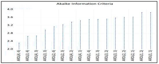
Figure 1.
Akaike information criteria.
According to the above diagram, the optimal model is ARDL (4,4). Given the presence of cointegration, we present both the long-run and short-run results of the ARDL (4,4) panel model in Table 9 and Table 10, respectively, with the optimal lag length using the Akaike information criterion.
Table 9.
Long-run results of panel ARDL (PMG).
Table 10.
Short-run results of panel ARDL (PMG).
Pesaran et al. [18] suggested two estimation procedures for solving the heterogeneity bias caused by heterogeneous slopes on dynamic panel coefficients. The Mean Group (MG) and the Pooled Mean Group (PMG) allow for a higher heterogeneity rank of the parameters in growth regressions.
The Mean Group (MG) estimator has the least limited process and allows for the heterogeneity of all coefficients, constant and slopes, with the estimation of a separate equation for each country, whereas the coefficients for the panel are calculated as non-weighted means of the other coefficients. The Mean Group (MG) estimator exports all the long-run parameters from the ARDL models for individual countries. Moreover, the MG estimator estimates separate regressions for each country. However, it calculates the means of the coefficients by country, which provides consistent estimations of the long-run coefficients.
The Pooled Mean Group (PMG) considers a lower heterogeneity level, as it establishes homogeneity on long run coefficients while still allowing heterogeneity for short-run coefficients and error variances.
The long-run results of ARDL (4,4) in Table 9 demonstrate that expenditures on research and development—R&D was found to have a significant positive relation with the global innovation index—GII for EU countries. This result suggests that an increase in expenditures on research and development by 1% leads to an increase in the global innovation index by 0.643%. This long-run result is confirmed by [19] for the 103 EU regions, [20] for the 20 OECD economies, [22] for the 11 selected EU countries and [23] for the three main indicators of innovation in European countries.
Regarding the short-run results of Table 10, we found that an increase in research and development expenditure by 1% in EU countries reduces the global innovation index by 0.52% at the 1% level of significance. The variable of error correction, which represents the speed of adjustment from short-run to long-run equilibrium, is negative and statistically significant at the 1% level of significance. The speed of adjustment, which is approximately 0.66%, is regarded as satisfying for the long-run equilibrium.
In Appendix C, the short-run results of the panel ARDL models are presented together with the dynamic panels. The Pooled Mean Group (PMG) allowed for a higher heterogeneity level of regression parameters for each EU country. The results in Appendix C show that, in countries such as Cyprus, Estonia, Lithuania and Poland, an increase in research and development expenditure raise the global innovation index, and the rest of the EU countries reduce the GI index in all countries except the Netherlands and Poland, which are significant at the 5% level; Greece, which is significant at the 10% level; and Cyprus, which is not statistically significant. This result can be explained by the share of innovative companies in EU countries, which has decreased in recent years due to COVID-19.
6.3. Panel Causality Test
The causality relationship between series was analyzed following the two-step technique of [46]. The first step contains the estimation of the long-run model for variables’ levels in order to create the estimated residuals according to the following function:
The second step consists of the use of residuals with a one-time lag from the above function as an error correction term in an ARDL panel system that is used for short- and long-run multivariable Granger causality. Multi-variable Granger causality allows us to include as additional control variables the differenced lagged values of all variables in the error correction ARDL model [45].
This system is expressed in the following equations:
Short-run Granger causality is jointly tested for the restricted coefficients with the F Wald distribution, whereas long-run causality is tested using the significance of the coefficient of error correction term. In the following Table 11, the results of short- and long-run Granger causality are provided.
Table 11.
Multivariate Granger causality test results.
The results of the above table indicate that there is a short-run and long-run causal relationship between research and development and the global innovation index for EU countries.
6.4. Impulse Response Functions
Based on the cointegration analysis, we used the IRF analysis, establishing Cholesky factoring to measure the influences on variables’ values from innovation, derived from a shock on the system using the Standard Percentile Bootstrap model with a 95% level of significance with 999 bootstrap repetitions, as shown in Figure 2.
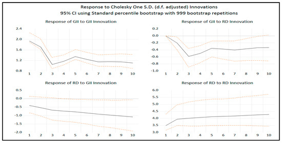
Figure 2.
Impulse response functions.
From the above diagram, we can notice that all the IRF estimated coefficients are within the estimated zones. The analysis of one variable shows that the impulse of one Cholesky standard deviation on an innovation term causes a change to another. Regarding the response to R&D expenditure, for the impact of the global innovation index on EU countries, the response in the current period is negative at −0.39. It decreases afterward, and in the second period it reaches −0.53. In the third period it is −0.68, and in the tenth period it is −1.08. Regarding the impact of the global innovation index of the response of R&D on EU countries, the response in the current period is zero until the third period, where there is a decrease that reaches −0.59. In the following two periods, there is a rise of −0.35 and a slight decrease of −0.40 in the next two periods. Up to period 10, there is a minimum increase of −0.33.
6.5. Variance Decomposition Analysis
The decomposition of variance is used to analyze the contribution of each structural impact on endogenous variables. Moreover, it is used for the assessment of the importance of different factors. The results of variance decomposition are presented in the following Table 12.
Table 12.
Variance decompositions results.
The results of variance decomposition show that the variances of global innovation on the same innovation represent 100% in the first period, and this percentage slowly reduces until the tenth period, reaching 92.5%. The percentage of expenditure on research and development is on a low level in the first period, but afterward, it increases rapidly to 7.47 until the last period. Among the factors that influence the variances of research and development expenditure, they represent 98.7% in the first period, and for innovation, they represent 1.25%. In the following periods, the shares change slightly and reach the tenth period with 96.15% and 3.89%, respectively. Finally, the average values of the results of variance decomposition show that the total variance for the global innovation is 94.5%, whereas for the expenditure of research and innovation, it is 97.34%.
7. Analysis of Results and Discussions
Innovation has a direct impact on the sustainability of economic growth in all EU countries, which is why it is vital to adopt policies that encourage investors to allocate more capital to research and development. The analysis of our paper shows that, as Ref. [29] found in the case of the Economies of Developing Countries, and Ref. [28] who examined the impact of innovation on the availability of cutting-edge technologies for 10 high-income countries, the impact of R&D spending is significant on the global innovation index.
The main purpose of this paper is to investigate the relationship between R&D expenditure and the global innovation index in EU countries for the period of 2007–2020 using a Panel Vector Autoregression model (PVAR). The PVAR model is not based on any a priori economic theory and treats all variables as endogenous. It also combines the traditional VAR methodology, taking all variables as endogenous, with a panel data technique that allows for unobserved individual heterogeneity. In addition, the PVAR model allows us to compute impulse response functions to estimate the magnitude of an exogenous shock for one of the endogenous variables and for all other variables over time.
From the descriptive statistics of the data, we observe that the average expenditure as a percentage of GDP for research and development in the 27 EU countries is USD 1.56 in constant 2015 prices and Purchasing Power Parities (PPPs), as a percentage of GDP, and the average global innovation index is 49.63. Subsequently, the panel data analysis with the Hausman test [46] helped us to select the fixed effects model as the most appropriate one. Moreover, the findings of the four tests of dependence rejected the null hypothesis of interlayer independence, as well as the homogeneity of the slopes. Pesaran’s [51] second-generation unit root test of CIPS [51], which takes into account interlayer dependence and heterogeneity, showed that the variables are zero I(0) and first-order I(1) integrated variables. Therefore, to test for cointegration, we use the vector autoregressive distributed lags (ARDL) model, as proposed by Ref. [36]. The cointegration results show that the null hypothesis of no cointegration is rejected. Given the presence of cointegration, we presented both the long-run and short-run effects of the ARDL (4.4) panel model with the optimal length of lags using the Akaike information criterion.
The long-run effect of the ARDL panel model (4.4) showed that research and development (R&D) expenditure was found to have a significant positive relationship with the global innovation index—GII in EU countries. The effect suggests that a 1% increase in R&D expenditure leads to an increase in the global innovation index of 0.643%. This long-run effect is also confirmed by the work of Refs. [14,15,17,18].
Regarding the short-run effects, we found that a 1% increase in R&D spending in EU countries reduces the global innovation index by 0.52% at the 1% level of significance. This result can be explained by the COVID-19 health crisis, which brought obstacles to the business activities of EU companies, different from the financial sector crisis in 2008 and 2009. For example, the most pressing problem in the first year of COVID-19 was mobility—travel restrictions, lockdown, border closures and disruption of the value chain (production and supply) [63]. The error correction variable, which represents the speed of adjustment from short- to long-run equilibrium, was negative and statistically significant at the 1% level. The speed of adjustment at around 0.66 % was considered satisfactory for the long-run equilibrium.
Also, the short-run effects of the ARDL panel models with dynamic panels Pooled Mean Group (PMG) coefficients, which allowed for a higher degree of heterogeneity of parameters in the regressions for each EU country, showed that increasing research and development expenditure increases the global innovation index in Cyprus, Estonia, Lithuania and Poland, while decreasing the global innovation index in the other EU countries. Innovation in times of recession is more important than ever. EU business growth was more affected by the COVID-19 pandemic than by the previous economic downturn in 2008 and 2009. Although both innovative and less innovative countries were affected by the COVID-19 crisis, this study showed that less innovative countries (Cyprus, Estonia, Lithuania and Poland) were not affected in the evolution of innovation by the COVID-19 crisis as most EU countries were. In other words, these findings suggest that innovation for these countries was more important than ever in mitigating the negative impact of the pandemic [53].
The long-run effect indicates a direct connection between R&D expenditure and the world innovation index in EU countries, whereas the short-run effect indicates that there could be an indirect connection between these variables in the short-run, but they always adjust back to equilibrium from the long-run effect.
The VECM panel causality analyses confirmed one-way short- and long-run causality from R&D expenditure to the global innovation index in EU countries.
Finally, the impulses of research and development spending on the impact of the global innovation index in the EU countries caused a downward effect. The impulses of global innovation caused a large decrease in the first three years, and then there was an upward trend until the tenth year.
8. Conclusions
Economic development is a tool for measuring the growth and progress of countries, and technological innovation is one of the factors that influence economic growth and contribute to the development and modernization of production methods. Spending on research and development and investing in innovation support competition and progress. In addition, they ensure a sustainable educational level of the workforce, create new products and improve people’s living conditions.
Innovation is one of the most important factors in a country’s growth and wealth. It is generally accepted that economically strong countries can afford and devote more funds to research and development. A strong economy allows for more innovation, which is recognized as the main driver for economic growth and human progress. In addition, sustainable economic growth ensures that resources are preserved for future generations and that economic and social development is achieved.
Europe maintains lofty ambitions for building its future development and prosperity and preserving its social model through innovation. In Lisbon in 2002, an ambitious target of devoting 3% of GDP to R&D by 2010 was set. The next strategy for 2020 defined a roadmap for sustainable and inclusive development growth. Despite this innovation-based strategy and R&D targeting, Europe’s innovation performance remains weak to date. According to the Innovation Union Scoreboard (IUS), developed by the European Commission, Europe is not performing well. Europe’s gap with the US holds true in almost all of the individual indicators included in the IUS score. Europe’s overall (public and private) R&D ratio to Europe’s GDP is currently below 2%, significantly lower than the figures in the US, Japan, South Korea and Singapore.
Looking at the heterogeneity between European countries, we find that some European countries are performing better than others (Table 13). The analysis found that Europe maintains an innovation system, with a few well-performing countries in which a slow process of convergence is taking place. Although integration has led to some level of convergence in innovation, the rate of convergence is slow. There are still significant differences between countries, not only in terms of the stock of knowledge but also in terms of the varying capacities to leverage knowledge into growth. To assess convergence, we look at the coefficient δ, i.e., the coefficient of variation . Convergence occurs when the dispersion in a group of economies decreases over time.
Table 13.
R&D as % of GDP.
As demonstrated in Table 13, the heterogeneity in R&D expenditure is significant, as shown by the variation coefficient.
In terms of innovation, the best performing countries are Sweden, the Netherlands, Finland, Denmark and Germany. The weakest group of countries includes most transition economies, including Bulgaria, Croatia, Romania and Poland. The level and structure of innovation should not be overlooked, as it plays a fundamental role in stimulating economic growth. EU countries with a high rate of investment in research and technology are very innovative and highly developed. The rest of the EU countries need to spend more on educational infrastructure so that innovation can deliver the expected results. Innovation has always been the focus of the technology industries in Europe. In the midst of the fourth industrial revolution, European industries have the opportunity to become global leaders by combining business and information technologies. The cornerstone of this innovative force is applied industrial research and development (R&D). Applied research applies the knowledge of basic scientific research in practice in a real-world environment. Moreover, it strengthens Europe’s global competitiveness and reinforces the high value-added industrial ecosystem.
The contribution of this work is fourfold. First, it uses the PVAR method, which combines the traditional VAR methodology, taking all variables as endogenous with a panel data technique that allows for unobserved individual heterogeneity. Second, unlike other work, the empirical analysis uses a panel time series autoregressive distributed lag (ARDL) model, as suggested by Ref. [61] as well as Ref. [42]. Therefore, the PVAR model is based on data and is therefore appropriate for analyzing the relationships between variables. In addition, through a panel ARDL model, we identified the short-run and long-run effects of research and development expenditure with the global innovation index in EU countries. The estimation procedures were performed by the Mean Group (MG) and the Pooled Mean Group (PMG) estimators, as solutions to heterogeneity bias caused by heterogeneous gradients in dynamic panels coefficients. Third, the causality test was performed with an ARDL error correction model, as proposed by [45]. Fourth, based on the cointegration analysis, we used impulse response function (IRF) analysis by imposing Cholesky factorization to measure the effects on the values of innovation variables caused by a shock to the system using the Standard Percentile Bootstrap method. In addition, variance decomposition was used to analyze the contribution of each structural impact to the endogenous variables. Finally, in contrast to other work, our research enhances our understanding of the relationship between research and development expenditure and the global index of innovation in EU countries.
The limitations of this research are as follows:
- There was a lack of data for more years, especially in new EU countries; therefore, we used annual data for the period of 2007–2020 (sample available in the sources for all EU countries).
- Economic growth has become the decisive element in all aspects of economic activity, as knowledge and innovation are the basis for economic and social development for all EU countries. Therefore, economic activities can be divided into sectors to examine their impact on innovation.
Therefore, future research should look at how to direct economic resources of EU countries toward knowledge industries in a manner that is equivalent to investments to various sectors, such as sustainable development, environment, health, education, industry, tourism and information technology. In addition, there is a need for ways to support researchers in the field of knowledge technologies and to increase the volume of expenditure on scientific research as a percentage of GDP, which has a positive impact on the economies of EU countries.
Based on the results of this study, the following recommendations can be made:
- Strategies should be adopted to improve high-tech in the countries of the weak group of countries shown in Table 13.
- In the same group of countries, governments should provide appropriate funding for research and development.
- Several EU countries should import technology from developed countries that may not suit their environment and thus cannot benefit from the technological innovation that is expected to be achieved.
- Finally, work should be carried out to create an environment that is conducive to innovation in all EU countries by expanding research and development spending and protecting intellectual property rights.
Author Contributions
Conceptualization, M.D. and C.D.; methodology, M.D.; software, C.D. validation, M.D., C.D.; formal analysis, M.D.; resources, C.D.; data curation, C.D.; writing—original draft preparation, M.D.; writing—review and editing, C.D.; All authors have read and agreed to the published version of the manuscript.
Funding
This research received no external funding.
Institutional Review Board Statement
Not applicable.
Informed Consent Statement
Not applicable.
Data Availability Statement
Not applicable.
Conflicts of Interest
The authors declare no conflict of interest.
Appendix A

Figure A1.
Research and development (R&D) expenditures to GDP ratio in EU countries.

Figure A2.
Research and development (R&D) expenditures to GDP ratio in EU countries.

Figure A3.
Research and development (R&D) expenditures to GDP ratio in EU countries.

Figure A4.
Global innovation index (GII) in EU countries.

Figure A5.
Global innovation index (GII) in EU countries.

Figure A6.
Global innovation index (GII) in EU countries.
Appendix B
Table A1.
Description of statistics of R&D and GII.
Table A1.
Description of statistics of R&D and GII.
| Economies Variables | Austria (AUT) | Belgium (BEL) | Bulgaria (BGR) | |||
|---|---|---|---|---|---|---|
| R&D | GII | R&D | GII | R&D | GII | |
| Mean | 2.89 | 53.68 | 2.43 | 53.06 | 0.67 | 40.68 |
| Maximum | 3.20 | 63.71 | 3.47 | 62.14 | 0.95 | 46.57 |
| Minimum | 2.41 | 50.13 | 1.85 | 49.05 | 0.43 | 30.28 |
| Std Dev | 0.25 | 3.77 | 0.47 | 4.17 | 0.16 | 3.51 |
| Skewness | −0.59 | 1.72 | 0.84 | 1.26 | 0.01 | −1.67 |
| Kurtosis | 1.92 | 4.97 | 2.90 | 3.47 | 1.78 | 7.02 |
| J–B | 1.49 | 9.23 | 1.67 | 3.89 | 0.86 | 16.01 |
| Cyprus (CYP) | Czech Republic (CZE) | Germany (DEU) | ||||
| Mean | 0.52 | 46.76 | 1.67 | 49.58 | 2.87 | 59.26 |
| Maximum | 0.82 | 51.51 | 1.99 | 53.85 | 3.16 | 71.28 |
| Minimum | 0.38 | 39.11 | 1.23 | 44.28 | 2.46 | 54.89 |
| Std Dev | 0.12 | 2.89 | 0.28 | 2.27 | 0.20 | 5.06 |
| Skewness | 1.31 | −1.15 | −0.49 | −0.42 | −0.34 | 1.66 |
| Kurtosis | 3.85 | 4.84 | 1.62 | 3.72 | 2.53 | 4.32 |
| J–B | 4.45 | 5.07 | 1.68 | 0.73 | 0.40 | 7.52 |
| Denmark (DNK) | Spain (ESP) | Estonia (EST) | ||||
| Mean | 2.92 | 59.50 | 1.28 | 48.76 | 1.55 | 50.93 |
| Maximum | 3.09 | 67.42 | 1.40 | 54.42 | 2.30 | 55.30 |
| Minimum | 2.51 | 56.42 | 1.19 | 43.81 | 1.05 | 44.57 |
| Std Dev | 0.14 | 3.43 | 0.06 | 2.68 | 0.34 | 2.57 |
| Skewness | −1.76 | 1.69 | 0.39 | 0.50 | 0.84 | −0.77 |
| Kurtosis | 6.14 | 4.40 | 1.97 | 3.50 | 2.99 | 4.02 |
| J–B | 13.05 | 7.82 | 0.98 | 0.74 | 1.65 | 2.01 |
| Finland (FIN) | France (FRA) | Greece (GRC) | ||||
| Mean | 3.18 | 60.18 | 2.19 | 54.96 | 0.90 | 39.66 |
| Maximum | 3.73 | 66.59 | 2.35 | 62.14 | 1.49 | 50.57 |
| Minimum | 2.72 | 55.10 | 2.02 | 49.25 | 0.57 | 34.18 |
| Std Dev | 0.37 | 3.01 | 0.08 | 3.76 | 0.29 | 4.10 |
| Skewness | 0.11 | 0.62 | −0.58 | 0.82 | 0.64 | 1.38 |
| Kurtosis | 1.49 | 3.22 | 3.84 | 2.74 | 2.22 | 4.83 |
| J–B | 1.34 | 0.94 | 1.22 | 1.63 | 1.30 | 6.44 |
| Croatia (HRV) | Hungary (HUN) | Ireland (IRL) | ||||
| Mean | 0.86 | 40.44 | 1.26 | 45.37 | 1.37 | 57.21 |
| Maximum | 1.24 | 46.85 | 1.60 | 50.57 | 1.61 | 61.42 |
| Minimum | 0.73 | 37.00 | 0.95 | 41.14 | 1.17 | 52.28 |
| Std Dev | 0.14 | 2.71 | 0.19 | 2.93 | 0.18 | 2.73 |
| Skewness | 1.59 | 0.71 | −0.00 | 0.12 | 0.12 | −0.29 |
| Kurtosis | 4.75 | 3.21 | 2.20 | 1.99 | 1.21 | 2.31 |
| J–B | 7.69 | 1.21 | 0.36 | 0.62 | 1.89 | 0.47 |
| Italy (ITA) | Lithuania (LTU) | Luxembourg (LUX) | ||||
| Mean | 1.30 | 46.67 | 0.91 | 42.26 | 1.31 | 56.50 |
| Maximum | 1.53 | 52.14 | 1.15 | 49.14 | 1.58 | 62.57 |
| Minimum | 1.12 | 40.69 | 0.78 | 38.49 | 1.12 | 50.84 |
| Std Dev | 0.11 | 2.72 | 0.11 | 3.27 | 0.16 | 3.43 |
| Skewness | 0.24 | −0.08 | 0.62 | 1.17 | 0.66 | 0.27 |
| Kurtosis | 2.18 | 3.56 | 2.63 | 3.52 | 1.90 | 2.45 |
| J–B | 0.52 | 0.20 | 0.97 | 3.37 | 1.72 | 0.34 |
| Latvia (LVA) | Malta (MLT) | Netherlands (NLD) | ||||
| Mean | 0.60 | 43.85 | 0.62 | 50.49 | 1.99 | 61.02 |
| Maximum | 0.71 | 47.00 | 0.80 | 56.10 | 2.29 | 66.28 |
| Minimum | 0.43 | 38.14 | 0.50 | 40.28 | 1.62 | 56.31 |
| Std Dev | 0.08 | 2.54 | 0.09 | 3.76 | 0.23 | 2.99 |
| Skewness | −0.61 | −0.75 | 0.49 | −1.30 | −0.47 | 0.11 |
| Kurtosis | 2.38 | 2.89 | 2.09 | 5.12 | 1.58 | 2.32 |
| J–B | 1.08 | 1.32 | 1.03 | 6.59 | 1.69 | 0.29 |
| Poland (POL) | Portugal (PRT) | Romania (ROU) | ||||
| Mean | 0.92 | 41.04 | 1.38 | 47.56 | 0.47 | 38.78 |
| Maximum | 1.39 | 46.85 | 1.61 | 51.89 | 0.52 | 46.10 |
| Minimum | 0.56 | 36.14 | 1.12 | 42.45 | 0.38 | 34.85 |
| Std Dev | 0.25 | 2.62 | 0.13 | 3.18 | 0.04 | 2.89 |
| Skewness | 0.37 | 0.49 | 0.10 | −0.19 | −0.73 | 1.12 |
| Kurtosis | 2.18 | 3.59 | 2.47 | 1.62 | 3.21 | 3.97 |
| J–B | 0.71 | 0.76 | 0.19 | 1.19 | 1.29 | 3.53 |
| Slovak Republic (SVK) | Slovenia (SVN) | Sweden (SWE) | ||||
| Mean | 0.75 | 43.14 | 2.07 | 47.16 | 3.29 | 63.48 |
| Maximum | 1.16 | 51.28 | 2.56 | 54.28 | 3.52 | 69.28 |
| Minimum | 0.44 | 39.05 | 1.42 | 40.14 | 3.10 | 55.71 |
| Std Dev | 0.20 | 3.36 | 0.33 | 3.53 | 0.12 | 3.29 |
| Skewness | −0.03 | 1.46 | −0.19 | 0.05 | 0.41 | −0.23 |
| Kurtosis | 2.53 | 4.31 | 2.37 | 3.05 | 2.28 | 4.12 |
| J–B | 0.12 | 6.02 | 0.31 | 0.01 | 0.68 | 0.87 |
Appendix C
Cross-section short-run coefficient. * indicates the level of significance at 1%.


References
- Baden-Fuller, C.; Haefliger, S. Business models and technological innovation. Long Range Plan. 2013, 46, 419–426. [Google Scholar] [CrossRef]
- OECD/European Union. Chapter 7. Measuring external factors influencing innovation in firms. In OSLO MANUAL, Guidelines for Collecting, Reporting and Using Data on Innovation, 4th ed.; OECD Publishing: Paris, France, 2018; pp. 145–162. [Google Scholar] [CrossRef]
- O’Reilly, C.; Binns, A.J.M. The three stages of disruptive innovation: Idea generation, incubation, and scaling. Calif. Manag. Rev. 2019, 61, 49–71. [Google Scholar] [CrossRef]
- Sözen, I.; Tufaner, M.B. The relationship between R&D expenditures and innovative development: A panel data analysis for selected OECD countries. Marmara Üniversitesi İktisadi İdari Bilim. Derg. 2019, 41, 493–502. [Google Scholar]
- European Commission. 2018. Available online: https://commission.europa.eu (accessed on 12 March 2023).
- Najjar, M.; Alsurakji, I.H.; El-Qanni, A.; Nour, A.I. The role of blockchain technology in the integration of sustainability practices across multitier supply networks: Implications and potential complexities. J. Sustain. Financ. Invest. 2023, 13, 744–762. [Google Scholar] [CrossRef]
- Anderson, J.C.; Narus, J.A. Business marketing: Understand what customers value. Harv. Bus. Rev. 1998, 76, 53–65. [Google Scholar]
- Al Momani, K.M.K.; Jamaludin, N.; Abdullah, W.Z.W.Z.W.; Nour, A.-N.I.-H. The influence of relational capital on the relationship between intellectual capital and earnings per share in the digital economy in the Jordanian industrial sector. In The Big Data-Driven Digital Economy: Artificial and Computational Intelligence; Springer: Cham, Switzerland, 2021; pp. 59–76. [Google Scholar] [CrossRef]
- Wu, Y.; Gu, F.; Ji, Y.; Guo, J.; Fan, Y. Technological capability, eco-innovation performance, and cooperative R&D strategy in new energy vehicle industry: Evidence from listed companies in China. J. Clean. Prod. 2020, 261, 121–157. [Google Scholar]
- Markham, S.K.; Ward, S.J.; Aiman-Smith, L.; Kingon, A.I. The valley of death as context for role theory in product innovation. J. Prod. Innov. Manag. 2010, 27, 402–417. [Google Scholar] [CrossRef]
- Sarpong, D.; Boakye, D.; Ofosu, G.; Botchie, D. The three pointers of research and development (R&D) for growth-boosting sustainable innovation system. Technovation 2022, 122, 102581. [Google Scholar] [CrossRef]
- Ortega-Argilés, R.; Potters, L.; Vivarelli, M. R&D and productivity: Testing sectoral peculiarities using micro data. Empir. Econ. 2011, 41, 817–839. [Google Scholar]
- Science Business Network. 2021. Available online: https://sciencebusiness.net (accessed on 12 March 2023).
- Baregheh, A.; Rowley, J.; Sambrook, S. Towards a multidisciplinary definition of innovation. Manag. Decis. 2009, 47, 1323–1339. [Google Scholar] [CrossRef]
- Fagerberg, J.; Verspagen, B. Technology-gaps, innovation-diffusion and transformation: An evolutionary interpretation. Res. Policy 2002, 31, 1291–1304. [Google Scholar] [CrossRef]
- Chudnovsky, D.; Lopez, A.; Pupato, G. Innovation and Productivity: A Study of Argentine Manufacturing Firms’ Behavior (1992–2001); Working Papers; Universidad de San Andres, Departamento de Economia: Buenos Aires, Argentina, 2004; Volume 70. [Google Scholar]
- Das, R.C. Interplays among R&D spending, patent and income growth: New empirical evidence from the panel of countries and groups. J. Innov. Entrep. 2020, 9, 18. [Google Scholar]
- Pesaran, M.H.; Shin, Y.; Smith, R.J. Pooled mean group estimation of dynamic heterogeneous panels. J. Am. Stat. Assoc. 1999, 94, 621–634. [Google Scholar] [CrossRef]
- Bilbao-Osorio, B.; Rodríguez-Pose, A. From R&D to innovation and economic growth in the EU. Growth Change 2004, 35, 434–455. [Google Scholar]
- Ulku, H. R&D, Innovation, and Economic Growth: An Empirical Analysis; IMF Working Paper; No. 04/185; International Monetary Fund, Research Department: Washington, DC, USA, 2004. [Google Scholar]
- Hasan, I.; Tucci, C.L. The innovation–economic growth nexus: Global evidence. Res. Policy 2010, 39, 1264–1276. [Google Scholar] [CrossRef]
- Gocer, I.; Alatas, S.; Peker, O. Effects of R&D and innovation on income in EU countries: New generation panel cointegration and causality analysis. Theor. Appl. Econ. 2016, 23, 153–164. [Google Scholar]
- Kacprzyk, A.; Doryń, W. Innovation and economic growth in old and new member states of the European Union. Econ. Res.-Ekon. Istraživanja 2017, 30, 1724–1742. [Google Scholar] [CrossRef]
- Aynur, P. Innovation and economic growth in developing countries: Empirical implication of Swamy’s random coefficient model (RCM), 3rd World Conference on Technology, Innovation and Entrepreneurship (WOCTINE). Procedia Comput. Sci. 2019, 158, 1122–1130. [Google Scholar]
- Kolodziejczyk, B.P. Innovation in Europe: A Comparative Study. Master’s Thesis, Department of Political Science, Centre for European Studies, University of Gothenburg, Gothenburg, Sweden, 2020. [Google Scholar]
- Omri, A. Technological innovation and sustainable development: Doe the stage of development matter? Environ. Impact Assess. Rev. 2020, 83, 106398. [Google Scholar] [CrossRef]
- Minović, J.; Jednak, S. The Relationship Between Innovation, Foreign Direct Investment and Economic Growth in the Selected EU and EU Candidate Countries. In Finance, Innovation and Technology: New Models and Structures; Institute of Economics—Ss. Cyril & Methodius University: Skopje, North Macedonia, 2021; pp. 96–115. ISBN 978-608-4519-23-2. [Google Scholar]
- Uğurluay, K.; Kirikkaleli, D. Sustainable technology in high-income economies: The role of innovation. Sustainability 2022, 14, 3320. [Google Scholar] [CrossRef]
- Mohamed, M.M.A.; Liu, P.; Nie, G. Causality between Technological Innovation and Economic Growth: Evidence from the Economies of Developing Countries. Sustainability 2022, 14, 3586. [Google Scholar] [CrossRef]
- Bera, A.K.; Jarque, C.M. Efficient tests for normality, homoscedasticity and serial independence of regression residuals: Monte Carlo Evidence. Econ. Lett. 1981, 7, 313–318. [Google Scholar] [CrossRef]
- Holtz-Eakin, D.; Newey, W.; Rosen, H.S. Estimating vector autoregressions with panel data. Econometrica 1988, 56, 1371–1395. [Google Scholar] [CrossRef]
- Love, I.; Zicchino, L. Financial development and dynamic investment behavior: Evidence from Panel VAR. Q. Rev. Econ. Financ. 2006, 46, 190–210. [Google Scholar] [CrossRef]
- Grossmann, A.; Love, I.; Orlov, A.G. The dynamics of exchange rate volatility: A panel VAR approach. J. Int. Financ. Mark. Inst. Money 2014, 33, 1–27. [Google Scholar] [CrossRef]
- Xing, X.; Ye, A. Consumption upgrading and industrial structural change: A general equilibrium analysis and empirical test with low-carbon green transition constraints. Sustainability 2022, 14, 13645. [Google Scholar] [CrossRef]
- Nickell, S. Biases in dynamic models with fixed effects. Econometrica 1981, 49, 1417–1426. [Google Scholar] [CrossRef]
- Karna, A.; Mavrovitis, C.; Richter, A. Disentangling reciprocal relationships between R&D intensity, profitability and capital market performance: A panel VAR analysis. Long Range Plan. 2022, 55, 102247. [Google Scholar]
- Lütkepohl, H. New Introduction to Multiple Time Series Analysis; Springer: Berlin, Germany, 2005. [Google Scholar]
- Wu, O.Q.; Chen, H. Optimal control and equilibrium behavior of production-inventory systems. Manag. Sci. 2010, 56, 1362–1379. [Google Scholar] [CrossRef]
- Zhang, Y.; Chen, H.; He, Z. Environmental regulation, R&D investment, and green technology innovation in China: Based on the PVAR model. PLoS ONE 2022, 17, e0275498. [Google Scholar]
- Stock, J.H.; Watson, M.W. Vector autoregressions. J. Econ. Perspect. 2001, 15, 101–115. [Google Scholar] [CrossRef]
- Wang, Q.; Zhang, F.; Li, R. Revisiting the environmental kuznets curve hypothesis in 208 counties: The roles of trade openness, human capital, renewable energy and natural resource rent. Environ. Res. 2023, 216, 114637. [Google Scholar] [CrossRef]
- Pesaran, M.H.; Shin, Y.; Smith, R.J. Bounds testing approaches to the analysis of level relationships. J. Appl. Econom. 2001, 16, 289–326. [Google Scholar] [CrossRef]
- Granger, C.W.J. Investigating causal relations by econometric models and cross spectral methods. Econometrica 1969, 37, 424–438. [Google Scholar] [CrossRef]
- Dumitrescu, E.-I.; Hurlin, C. Testing for Granger non-causality in heterogeneous Panels. Econ. Model. 2012, 29, 1450–1460. [Google Scholar] [CrossRef]
- Mawejje, Μ.; Odhiambo, Ν.Μ. Macroeconomic determinants of fiscal policy in East Africa: A panel causality analysis. J. Econ. Financ. Adm. Sci. 2021, 27, 105–123. [Google Scholar] [CrossRef]
- Engle, R.F.; Granger, C.W.J. Co-integration and error correction: Representation, estimation, and testing. Econometrica 1987, 55, 251–276. [Google Scholar] [CrossRef]
- Liu, C.; Xia, G. Research on the dynamic interrelationship among R&D investment, technological innovation, and economic growth in China. Sustainability 2018, 10, 4260. [Google Scholar]
- Hamilton, J.D. Time Series Analysis; Princeton University Press: Princeton, NJ, USA, 1994. [Google Scholar]
- Wu, M.; Zhao, M. Dynamic relations between energy consumption, environmental pollution and economic growth—Based on China’s 1990–2014 time series data. Res. Technol. Econ. Manag. 2016, 12, 25–29. [Google Scholar]
- Baltagi, B.H. Econometric Analysis of Panel Data, 3rd ed.; Wiley: Chichester, UK, 2005. [Google Scholar]
- Dritsaki, C.; Dritsaki, M. Introduction in Econometrics; Klidarithmos Publications: Athens, Greece, 2020. [Google Scholar]
- Hausman, J.A. Specification tests in econometrics. Econometrica 1978, 46, 1251–1271. [Google Scholar] [CrossRef]
- Wang, Q.; Yang, T.; Li, R. Does income inequality reshape the environmental Kuznets curve (EKC) hypothesis? A nonlinear panel data analysis. Environ. Res. 2023, 216, 114575. [Google Scholar] [CrossRef]
- Breusch, T.S.; Pagan, A.R. The lagrange multiplier test and its applications to model specifications in econometrics. Rev. Econ. Stud. 1980, 47, 239–253. [Google Scholar] [CrossRef]
- Pesaran, M.H. General Diagnostic Tests for Cross Section Dependence in Panels; Cambridge Working Papers in Economics 0435; Department of Applied Economics, University of Cambridge: Cambridge, UK, 2004. [Google Scholar]
- Baltagi, B.H.; Feng, Q.; Kao, C. Testing for sphericity in a fixed effects panel data model. Econom. J. 2011, 14, 25–47. [Google Scholar] [CrossRef]
- Wang, Q.; Wang, X.; Li, R. Does urbanization redefine the environmental Kuznets curve? An empirical analysis of 134 Countries. Sustain. Cities Soc. 2022, 76, 103382. [Google Scholar] [CrossRef]
- Wang, Q.; Wang, L.; Li, R. Trade protectionism jeopardizes carbon neutrality–Decoupling and breakpoints roles of trade openness. Sustain. Prod. Consum. 2023, 35, 201–215. [Google Scholar] [CrossRef]
- Hsiao, C. Analysis of Panel Data, 3rd ed.; Cambridge University Press: Cambridge, UK, 2014. [Google Scholar]
- Pesaran, M.H. A simple panel unit root test in the presence of cross-section dependence. J. Appl. Econom. 2007, 22, 265–312. [Google Scholar] [CrossRef]
- Pesaran, M.H.; Shin, Y. An autoregressive distributed-lag modelling approach to cointegration analysis. In Econometrics and Economic Theory in the 20th Century: The Ragnar Frisch Centennial Symposium; Strøm, S., Ed.; Cambridge University Press (Econometric Society Monographs): Cambridge, UK, 1999; pp. 371–413. [Google Scholar]
- Akaike, H. A new look at the statistical model identification. IEEE Trans. Autom. Control 1974, 19, 716–723. [Google Scholar] [CrossRef]
- Khatib Saleh, F.A.; Nour, A.-N.I. The impact of corporate governance on firm performance during the COVID-19 pandemic: Evidence from Malaysia. J. Asian Financ. Econ. Bus. 2021, 8, 943–952. [Google Scholar] [CrossRef]
Disclaimer/Publisher’s Note: The statements, opinions and data contained in all publications are solely those of the individual author(s) and contributor(s) and not of MDPI and/or the editor(s). MDPI and/or the editor(s) disclaim responsibility for any injury to people or property resulting from any ideas, methods, instructions or products referred to in the content. |
© 2023 by the authors. Licensee MDPI, Basel, Switzerland. This article is an open access article distributed under the terms and conditions of the Creative Commons Attribution (CC BY) license (https://creativecommons.org/licenses/by/4.0/).