Article

Modeling Occupant Window Behavior in Hospitals—A Case Study in a Maternity Hospital in Beijing, China

1
Beijing Key Laboratory of Green Built Environment and Energy Efficient Technology, Beijing University of Technology, Beijing 100124, China
2
Key Laboratory for Comprehensive Energy Saving of Cold Regions Architecture of Ministry of Education, Jilin Jianzhu University, Changchun 130118, China
3
Faculty of Built Environment, Universiti Malaya, Kuala Lumpur 50603, Malaysia
4
Department of Mechanical Engineering, Faculty of Engineering, Universiti Malaya, Kuala Lumpur 50603, Malaysia
5
The Bartlett School of Sustainable Construction, University College London, London WC1E 7HB, UK
*
Author to whom correspondence should be addressed.
Sustainability 2023, 15(11), 8606; https://doi.org/10.3390/su15118606
Submission received: 11 January 2023 / Revised: 21 May 2023 / Accepted: 22 May 2023 / Published: 25 May 2023
(This article belongs to the Special Issue Sustainable Smart Cities and Society Development)

Abstract

:
Nowadays, relevant data collected from hospital buildings remain insufficient because hospital buildings often have stricter environmental requirements resulting in more limited data access than other building types. Additionally, existing window-opening behavior models were mostly developed and validated using data measured from the experimental building itself. Hence, their accuracy is only assessed by the algorithm’s evaluation index, which limits the model’s applicability, given that it is not tested by the actual cases nor cross-verified with other buildings. Based on the aforementioned issues, this study analyzes the window-opening behavior of doctors and patients in spring in a maternity hospital in Beijing and develops behavioral models using logistic regression. The results show that the room often has opened windows in spring when the outdoor temperature exceeds 20 °C. Moreover, the ward windows’ use frequency is more than 10 times higher than those of doctors’ office. The window-opening behavior in wards is more susceptible to the influence of outdoor temperature, while in the doctors’ office, more attention is paid to indoor air quality. Finally, by embedding the logistic regression model of each room into the EnergyPlus software to simulate the CO2 concentration of the room, it was found that the model has better applicability than the fixed schedule model. However, by performing cross-validation with different building types, it was found that, due to the particularity of doctors’ offices, the models developed for other building types cannot accurately reproduce the window-opening behavior of doctors. Therefore, more data are still needed to better understand window usage in hospital buildings and support the future building performance simulations of hospital buildings.

1. Introduction

The study of window-opening behavior can be traced back to the 20th century when Nicol et al. [1] proposed that natural ventilation can be provided using openable windows and other adaptive mechanisms. Natural ventilation is one of the most straightforward and healthy methods to enhance thermal comfort and air quality in indoor atmospheres [2]. Compared to mechanical ventilation, this approach uses less energy and is better for the indoor environment [3,4]. In naturally ventilated buildings, people frequently use windows to regulate the indoor temperature for thermal comfort and indoor air quality, especially during transitional seasons [5]. According to Li et al. [6], opening windows for just two minutes can provide sufficient fresh air needed for a standard room. Additionally, when all windows are open, the total ventilation rate may even be higher than that provided by mechanical ventilation [7]. However, the occupants’ window-opening behavior often exhibits significant randomness and uncertainty, leading to unreliable ventilation for the building [8]. This randomness/uncertainty also causes a significant performance gap between simulated and actual building performances, i.e., a performance gap. Therefore, capturing and understanding the dominant factors affecting occupants’ window-opening behavior is essential for accurate and efficient building design and operation [9].
In the early research, the method of collecting data for window-opening behaviors was to take photos of the window status at different times every day [10,11]. With the development of research, the means of collecting data have changed to conducting questionnaires with indoor personnel many times a day [12,13]. Until 2004, the monitoring of window-opening behaviors began to change from questionnaire surveys to sensor monitoring [14]. This measurement method is more convenient and can obtain real-time data for more accurate research. After that, lots of research on window-opening behavior began to appear. The types of buildings studied mainly focus on residential and office buildings. For example, Pan et al. [15] studied one university office building in China and reported that the opening and closing behaviors of windows is affected by working hours and environmental factors. It was found that people usually open/close windows when they arrive or leave their offices. Wei et al. [16] suggested that the window state at the end of the day was affected by factors such as season, office floor, gender, etc., according to the data collected from one office building in the UK. According to Yun et al. [17], these factors also affect occupants’ window-opening behavior during office hours. In particular, the influence of seasons has been observed as indicated by the fact that when the outdoor temperature is the same but in different seasons, the law of window-opening behavior also changes [18]. Yun et al. [19] also found that the window state after leaving the office also affected the window use in the office the next day. Furthermore, due to directional factors such as solar radiation and wind direction, window orientation may also affect window-opening behavior [20]. This can also be interpreted as the influence of environmental factors on window-opening behavior. Among all the environmental factors, indoor and outdoor air temperatures were reported as the most significant [15,16,17,18,19,20,21,22,23]. With the deepening of the related research in this area, the influence of other factors has been revealed, including indoor and outdoor relative humidity, PM2.5 concentration, indoor CO2 concentration, outdoor wind speed, etc. [5,15,23].
It is well acknowledged that residential buildings have different functions compared to office buildings, especially during resting and sleeping. Therefore, the time of day affects the window behavior in residential buildings differently from that of office buildings. In order to determine the typical window-opening schedule in Chinese residential buildings, Lai et al. [24] undertook one-year research across 58 apartments in 14 cities across five major climatic regions, and their results indicated that, on weekdays, approximately 40% of window-opening actions occurred between 6:00 and 9:00, and on weekends, window-opening behavior mainly occurred from 9:00 to 17:00. Additionally, more frequent window-opening action was found in families with people who did not need to leave their home to work. In terms of time-related factors, some daily activities in residential buildings differ from those in office buildings, such as cooking, cleaning, and getting fresh air, which accounted for 27%, 40%, and 33% of residential buildings’ window opening probability, respectively [25]. Additionally, regardless of the building type, occupants’ window-opening behavior is also affected by environmental factors, again with the ambient temperature as the major factor [26,27]. Besides temperature, the CO2 concentration also showed a significant influence [28,29,30]. In some studies, it has been found that the influence of CO2 concentration was even more significant than that of indoor and outdoor temperatures [31]. Furthermore, indoor and outdoor humidity, indoor and outdoor PM2.5 concentrations, solar radiation, etc., have also been considered as influential in residential window-opening behaviors [32,33].
Notably, comprehensive research on the window-opening behaviors of offices and residential buildings has been widely explored and acknowledged, and its law under the influence of environmental and non-environmental factors has been discussed in detail. However, research on window-opening behaviors in a hospital architecture has rarely been reported. A hospital is a special area with a large vulnerable population and multiple pollution sources [34,35]. Therefore, besides maintaining a high ventilation rate, it is essential to adjust hospital buildings’ internal ventilation reasonably [36]. Hence, it is undeniably necessary to study how doctors and patients operate their windows in hospitals and identify the major influential factors in these behaviors. Shi et al. [37] investigated the window-opening habits of two wards in a naturally ventilated general hospital in Nanjing, China. The study revealed seasonal differences in terms of window adjustments to environmental changes, i.e., the correlation between outdoor temperature and window opening probability was negative in the cooling season and positive in transitional and heating seasons. Their study, however, focused on the window-opening behaviors in hospital wards only, while ignoring the rooms where doctors were present, such as doctors’ offices and lounges. Compared to the wards, these rooms have different functions, and their main occupants also vary. These differences may lead to a considerable different window usages. Furthermore, the types of patients in the wards of different hospital types may also be different. For example, most wards in maternity hospitals are filled with pregnant women and newborns, who are more susceptible to environmental influences owing to their weaker immune systems [38,39]. Therefore, these wards are different from wards in other hospital buildings. Maternity hospitals need to design stricter criteria for air quality than general hospitals, and the particularity of their window-opening behaviors also needs further exploration. This study compares and evaluates the window-opening behaviors of maternity hospital wards, a doctors’ office, and a doctors’ lounge in spring, and uses the logistic regression method to model the window-opening behavior. As early as 1973, Humphreys [40] proposed using logical regression to predict the window-opening behavior. After that, more scholars used this algorithm to predict the window-opening behavior in buildings [41]. Logistic regression is one of the most commonly used modeling methods in the study of window-opening behavior to date, because it has irreplaceable advantages in accuracy and explanatory power [42]. Currently, the methods to evaluate the accuracy of the logistic regression model use a model evaluation algorithm that assesses the accuracy which has not been further applied to the actual scenario. Moreover, they are based on a proprietary prediction model corresponding to the initial building, which limits their generalization for different cases. Therefore, to study the logistic regression model, it is important to consider its applicability in the actual scene and the universality of the model [43]. In order to solve the above problems, this study embeds the logistic regression model of each room into the EnergyPlus software to simulate the indoor CO2 concentration in the room, and compares the simulation results to those of a fixed schedule. In addition, this study also uses spring data from a Beijing school office [15], an infant’s family home [8], and data from a doctors’ office to perform modelling and prediction, and additionally uses a residential model [44] to predict the window-opening behavior in the doctors’ office. Finally, different model evaluation indices are used to evaluate the errors between the training and verification datasets, hence assessing the model’s accuracy. This study supplements the deficiency of the research on window-opening behaviors in hospital buildings, verifies the applicability of the logistic regression model in actual scenarios and the generalization of prediction between different buildings, and provides ideas and methods to further promote the logistic regression model.

2. Research Method

2.1. Case Study Building

The case study is a maternity hospital located in Beijing, China. Three maternity wards located on the second floor of its inpatient department were selected, along with the doctors’ office and lounge on that floor. Reinforced concrete and thermal insulation materials make up the main construction of the building, and there are no high-rise buildings or trees around the building to obstruct solar radiation. Additionally, there is no significant outdoor noise issue either. Figure 1 shows the exterior façade of the case study building. Each room inside the building has openable external windows and is equipped with split air conditioners and radiators, as shown in Figure 2a,b. In the cooling season, the indoor split air conditioner is used for independent cooling. In the heating season, the central heating is used to dissipate heat indoors through radiators. In the transition season, the rooms rely on natural ventilation to improve the indoor environment. The investigated doctors’ office (with 8 occupants and 2 windows) and the three wards (2 rooms with 4 beds and 1 window, and a room with 2 beds and 1 window) are located on the northeast façade, and the doctors’ lounge (with 1 window) is symmetrically arranged on the southwest façade. Each patient in both wards is accompanied by two family members, whereas there is no vacant bed in the ward during the test. On the other hand, two doctors are allowed to rest in the lounge. The room marked with a red star in Figure 3 is the case study in this test. In transitional seasons, indoor air quality and thermal environment are mainly controlled by natural ventilation through manually opening/closing the room windows.

2.2. Data Collection

In the early stage of window-opening behavior research, scholars only paid attention to the influence of some thermal comfort parameters (mainly indoor and outdoor temperatures) on people to propose many models for these parameters [45]. With the development of research, scholars began to pay attention to other environmental factors, such as relative humidity, wind speed, and PM2.5 concentration. It was found from previous studies that these parameters will affect the window-opening behavior [15]. In this study, the measurement was carried out in the spring season of 2019, between 15 March and 15 May. The measured parameters included window state, indoor environmental parameters (i.e., temperature, relative humidity, and CO2 concentration), and outdoor environmental parameters (i.e., temperature, relative humidity, PM2.5 concentration, wind speed, and wind direction), as shown in Figure 4a–c. Table 1 lists some major technical specifications for the monitoring instruments used in this study. Before the field measurement, all instruments were calibrated to ensure accuracy. The outdoor weather station was placed on the roof of the case study building, while only the outdoor PM2.5 concentration was obtained from a close public weather station [46]. A window magnetic switch recorder was used to monitor the opening/closing state. This method is commonly used in existing studies [15]. In this study, the monitoring interval was set to 10 min for all environmental parameters, except for the outdoor PM2.5 concentration, where an interval of 1 h is used. Table 2 provides descriptive statistics for the environmental variables collected during the study period.

2.3. Statistical Analysis

Similarly to existing studies [47,48,49], this study adopted the logistic regression analysis to analyze window-opening behavior in buildings and examine the variables influencing maternity hospitals’ window-opening practices.
Before modeling, the F test in the analysis of variance (ANOVA) was used to test the relationship between the respective variables and the dependent variables. ANOVA is a statistical test to evaluate the significant difference between the mean values of specific measurements. If the p value is less than 0.05, it is considered that the independent variable has a significant influence on the dependent variable [5]. The calculation method is as follows:
F = M S B M S F = S S B ( r 1 ) S S E ( n r )
where SSB represents the sum of squares of deviations between the average value of each group of variables and the total average value, indicating the differences between groups; SSE represents the sum of the average value of each group of variables and the sum of the squares of the deviations of this group of variables, representing the intra-group differences; MSB and MSE are the mean square values obtained by dividing the inter-group SSB and the intra-group SSE by their respective degrees of freedom (inter-group r − 1 and intra-group nr, where n is the total number of samples and r is the number of groups).
Then there is the logistic regression model. In this study, the dependent variable is the window state (open/closed), not window-opening angle. Logit transformation makes the dependent or independent variables of the logistic regression model linearly predictable. Furthermore, the ratio of occurrence probability (P) to non-occurrence probability (1 − p) is known as odds, and its logarithm is known as the logit transformation [8]. It is denoted as logit, and the logistic regression function is represented by Equation (2) as follows:
logit p = ln p 1 p = α + i = 1 i β i x i
where α is a constant; βi is a regression coefficient that represents the contribution of xi to pi; xi is an explanatory variable independent of the window state; and p is the probability of the window opening under different explanatory variables.
Before the analysis, all related environmental parameters must be normalized by Equation (3) to compare the contributions of different explanatory variables.
x = x i x min x max x min
where x is the normalized explanatory variable; xi is the unprocessed explanatory variable; xmax is the maximum value of the explanatory variable; xmin is the minimum value of the explanatory variable.
The normalized parameters were then entered into the logistic regression model as input parameters. The statistical analysis was carried out using SPSS.26, a popular statistical analysis tool worldwide (IBM, Armonk, NY, USA).
After the logistic regression model is established, the energy management system (EMS) in EnergyPlus is used to add the window-opening behavior model to the building model to simulate the indoor CO2 concentration. The functions used are Sensor, Actuator, Program calling manager, and Program, where each function is responsible for the following work:
(1)
Sensor: defines the variable parameters (indoor temperature, indoor relative humidity, indoor CO2 concentration, outdoor temperature, outdoor humidity, outdoor PM2.5, outdoor wind speed, and wind direction) required for building the window model.
(2)
Actuator: defined as the name to determine the opening ratio of the dynamic windowing model. For example, the name of the opening ratio of the doctors’ office window is defined as W10W, where 1 represents a fully open case and 0 represents a fully closed case. Ventwin210 is the name of the opening rate defined in this model, and the opening rate is defined in Schedule: Constant, in which the opening rate is initially defined as 1.
(3)
Program calling manager: determines the time to run the dynamic window model. The model calling point selected in this study is ‘BeginNewEnvironment’. Hence, the dynamic window model is triggered before inputting new parameters.
(4)
Program: enters the dynamic window model. The model in EnergyPlus is defined such that when the result of the logistic regression model is greater than 0, the window opens; otherwise, the window is closed. The opening degree of this setting is half of the fully opened area. This is based on the feedback from the interviews with residents in the early stage of actual measurement, where they mentioned that half of the windows are usually open.

3. Results and Analysis

3.1. Preliminarily Statistical Analysis

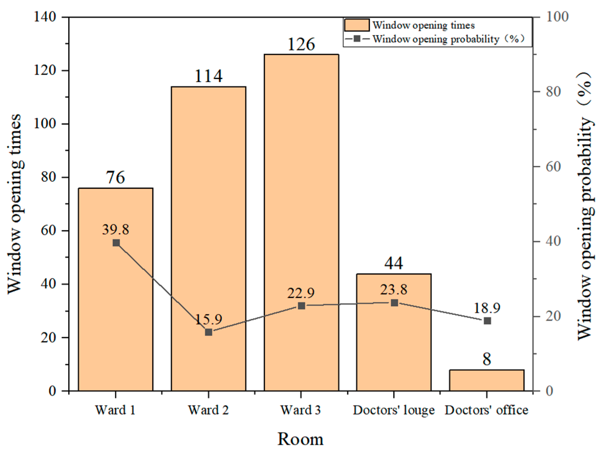
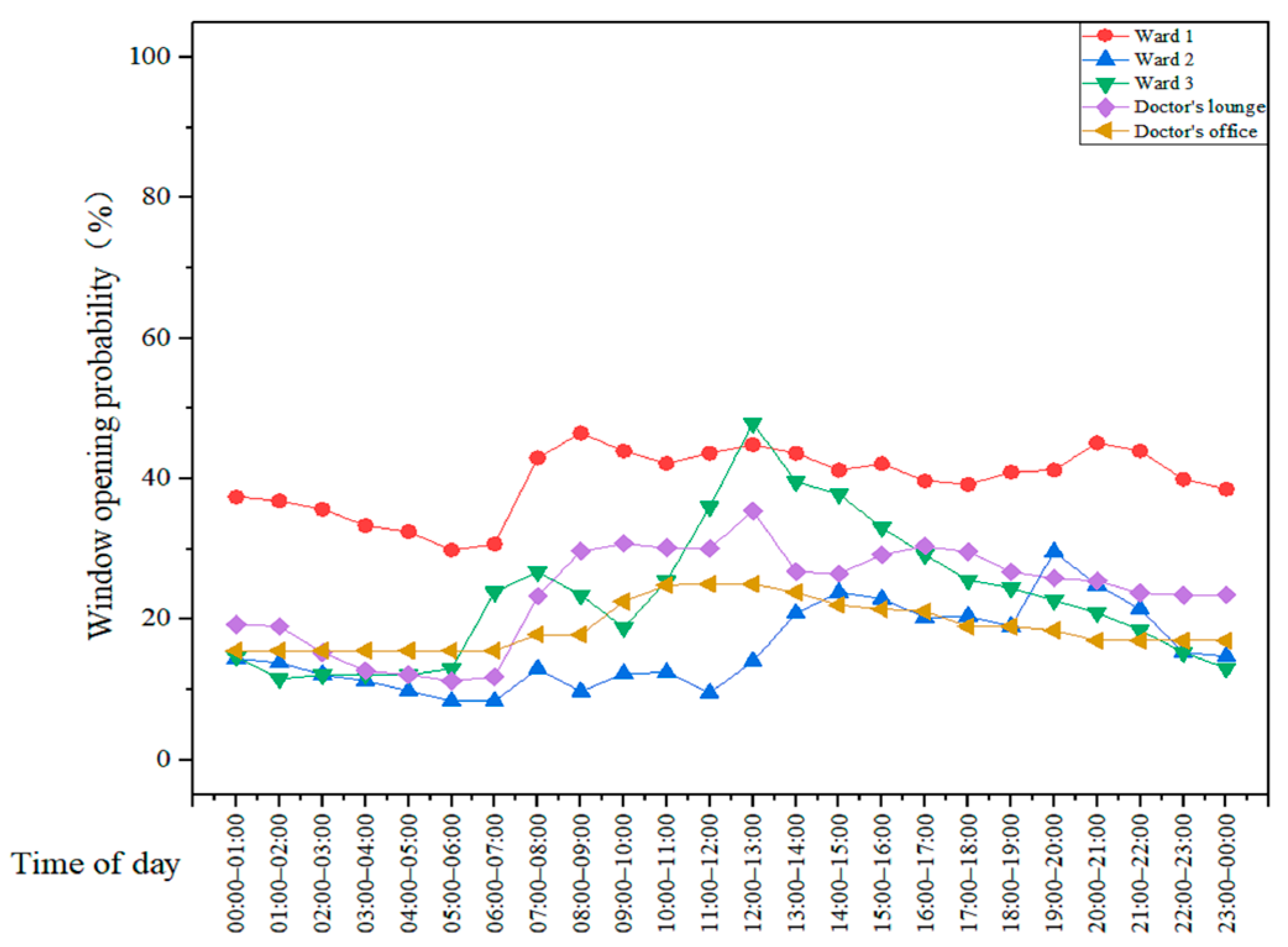
Figure 5 shows each room’s monitored window opening times and the calculated window opening probability. It can be observed that the times of window openings in the wards during the test are much higher than those in the doctors’ office and lounge. The window opening times in the doctors’ office were only 8 during the whole test period, which sharply contrasted with the 126 times in ward 3. Moreover, even though the window opening probability of ward 3 and that of the doctors’ lounge are similar, with a difference below 1%, the window opening times are far from each other. This shows that the patients are more sensitive to the change in environment as they will change the window state in time to ensure that the indoor environment is comfortable. Furthermore, it can be seen from the daily variation curve of the window opening probability (Figure 6) that doctors rarely change the state of windows many times in one day. Most of the time, the windows are either open or closed for a long time, especially in the doctors’ office. In addition, the window opening probability of all rooms only fluctuates in a small range in early spring, but after 17 April, the window opening probability of all rooms, including the doctors’ office, has significantly increased. By comparing the environmental parameters, it was found that the outdoor temperature obviously increased, and appears to be close to 20 °C for the first time. After that, the fluctuation range of the window opening probability of each room obviously increased, and the phenomenon of window opening all day began to appear. This also shows that the window-opening behavior is affected by the outdoor temperature. However, the existence of other factors affecting the window-opening behavior cannot only be found from the data observation. Hence, further statistical analysis is needed.

3.2. Outdoor Environmental Factors

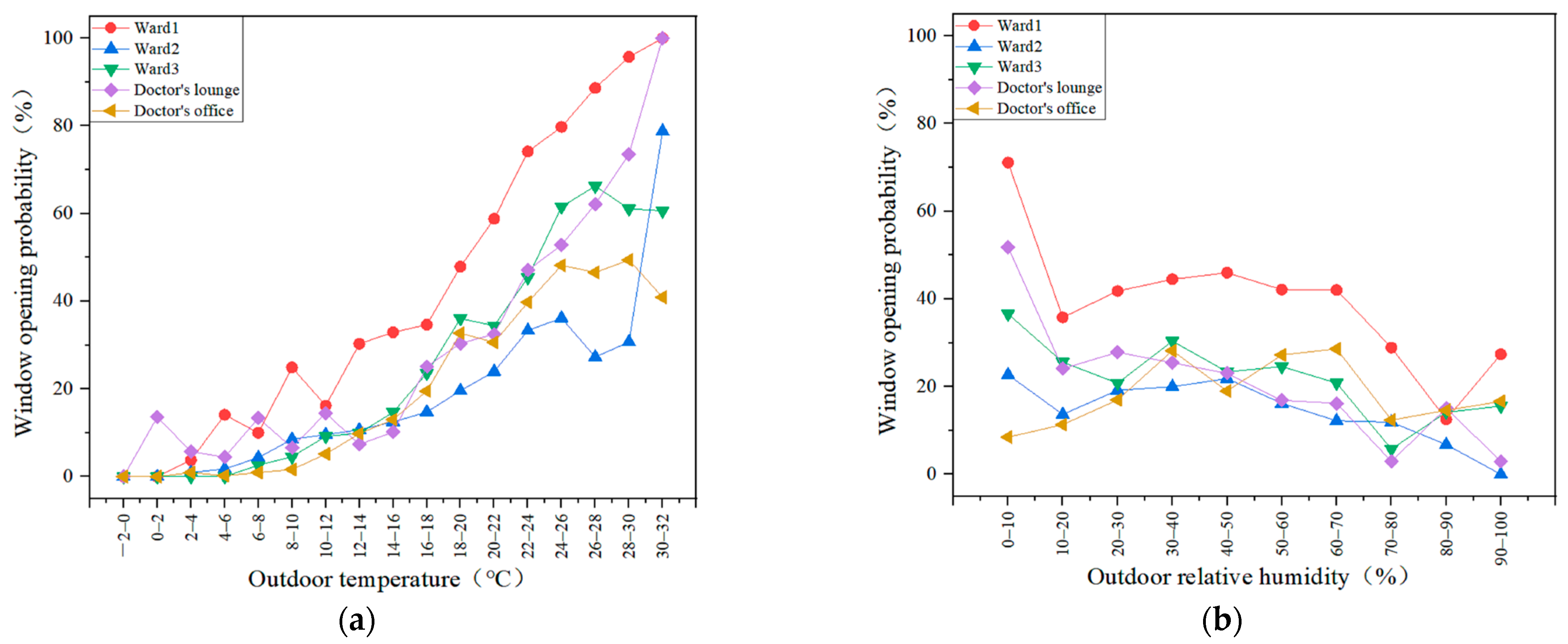
The above analysis shows that the outdoor temperature affects the window opening probability. Nevertheless, its changing rule regarding the outdoor temperature is still unclear. In addition, whether the window opening probability is affected by other environmental factors and the type of change rules that exist needs further statistical analysis. Therefore, this section first quantitatively analyzes the influence of outdoor environmental factors (temperature, relative humidity, PM2.5 concentration, wind speed, and wind direction) on the window-opening behavior in the wards, doctors’ office, and doctors’ lounge.
Figure 7a shows the relationship between the outdoor temperature and the window opening probability. In spring, the window opening probability is positively correlated with the outdoor temperature in the wards, doctors’ office, and doctors’ lounges. The window opening probability for the five rooms is consistent with the change in the outdoor temperature, but it can be seen from Figure 7b that, under the influence of outdoor relative humidity, the doctors’ office begins to show different rules compared to other rooms. As can be seen from the figure, when the outdoor relative humidity is in the range of 0–20%, the window opening probability of four rooms apart from the doctors’ office is inversely proportional to the outdoor relative humidity, with obvious fluctuations. The window opening probabilities for Ward 1, Ward 2, and the doctors’ lounge rebounded after more than 20%, and ward 3 began to rebound after more than 30%. In addition, the window opening probabilities for wards 1 and 2 kept rising after the rebound, and did not begin to decrease until the outdoor relative humidity exceeded 50%. However, the window opening probability of ward 3 and the doctors’ lounge began to decline immediately upon reaching 10% relative humidity. Unlike these rooms, when the relative humidity of the doctors’ office was less than 40%, the window opening probability was positively correlated to the outdoor relative humidity. The window opening probability was kept high in the range of 40–70% until the outdoor relative humidity exceeded 70%, and the window opening probability began to decline. This indicates that the doctors believe that 40–70% outdoor relative humidity range is suitable. Additionally, its outdoor relative humidity acceptance range is higher than other rooms compared to other rooms. This shows that, under the influence of outdoor relative humidity, the window-opening behavior for the doctors’ office varies from other rooms.
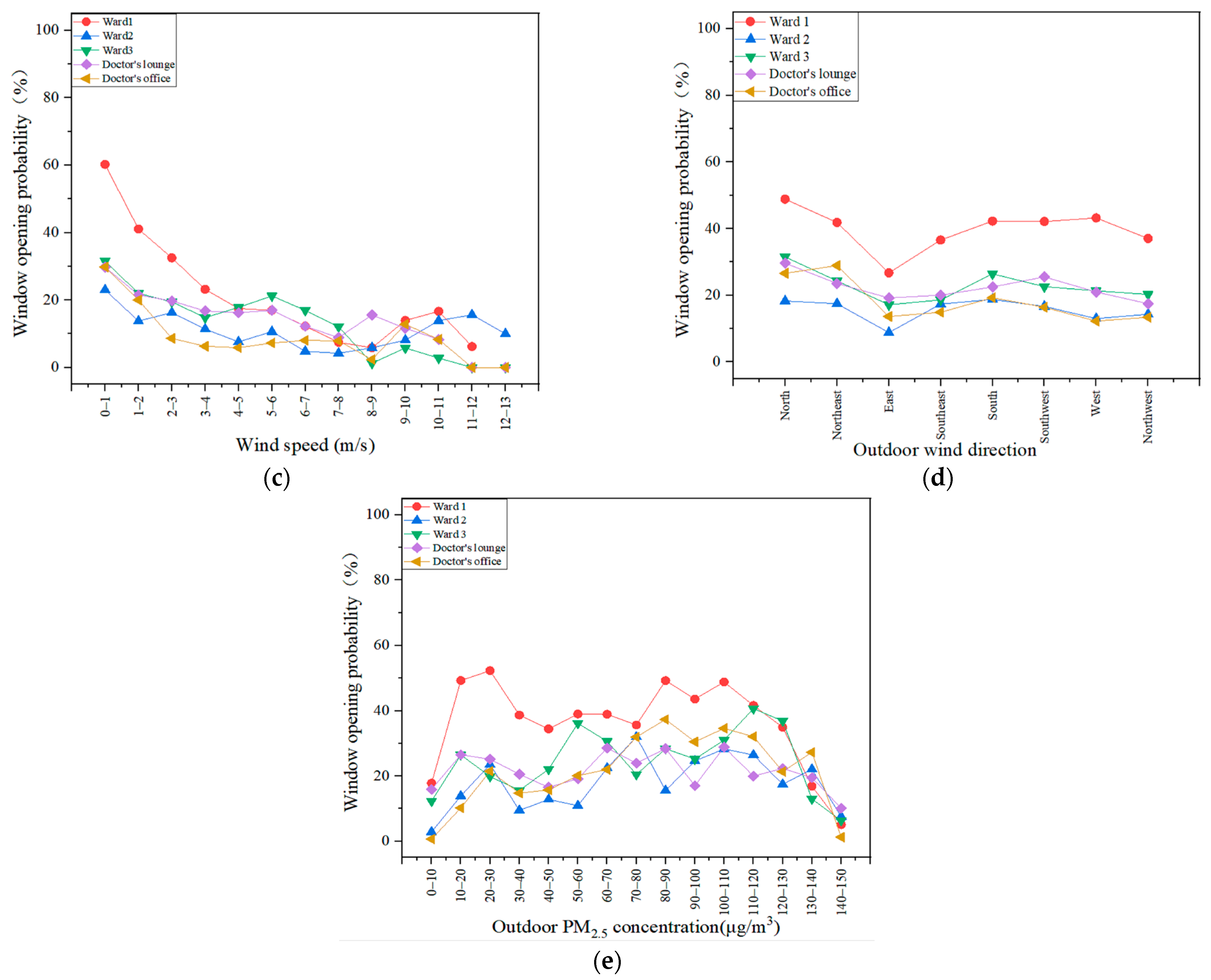
Figure 7c shows the relationship between the outdoor wind speed and window opening probability. As can be seen from the figure, the window opening probability of five rooms shows a consistent changing rule, where all of them are negatively correlated with outdoor wind speed. In addition, it is worth noting that the window opening probability’s variation law for the five tested rooms with the wind direction is the same (Figure 7d). However, logically speaking, the window orientations of the five tested rooms are different, and the influence of wind direction on the window opening probability of the room should have corresponding rules according to the window orientation. Hence, it is impossible to determine the reason from the curve analysis, which requires further combined modeling to analyze its impact.
Finally, an explanation of how outdoor PM2.5 levels influence window-opening behavior was provided (Figure 7e). Notably, PM2.5 is the source of several respiratory infections, particularly in children under five, and is a severe health hazard [8]. Therefore, more academics recently focused on how the PM2.5 concentration affects window-opening behavior [50]. According to China’s applicable specifications [51], when the concentration of PM2.5 exceeds 75 μg·m−3, it is considered mild environmental pollution. As can be seen from the figure, under the influence of outdoor PM2.5 concentration, the window opening probability’s change law for the five tested rooms also shows the same law. When the outdoor PM2.5 concentration is higher than 75 μg·m−3, the window opening probability will not immediately decrease until the PM2.5 concentration reaches 110 μg·m−3. This result can be attributed to the fact that the human body does not detect the slight environmental pollution caused by an increased PM2.5 concentration at its low concentration. Therefore, the premise of the PM2.5 concentration affecting the window-opening behavior is that its concentration must be greater than 110 g·m−3. This is because, when there is a high concentration of PM2.5 outdoors, it causes some visible environmental pollution, such as PM10.

3.3. Indoor Environmental Factors

Section 3.2 analyzes the influence of outdoor environmental factors and window-opening behavior and finds the difference between the doctors’ office and a room under the influence of outdoor relative humidity. Moreover, this section continues to analyze the influence of indoor environmental factors on the window-opening behavior.
Figure 8a shows that the window opening probabilities of the doctor’s room and ward vary under the influence of indoor temperature. First of all, from the indoor temperature range, the indoor temperature range of the ward is higher than the overall temperature range of the doctors’ lounge and office. Secondly, from the changing trend of the window opening probability, the doctors’ office and doctors’ lounge are positively correlated with the indoor temperature, while the ward shows a trend of first decreasing and then rising, and there is a minimum window opening probability. The lowest probability of opening a window means that the indoor temperature is comfortable in this temperature range. Hence, the window will not be opened to improve the indoor environment, while the doctor’s room does not have this range. It shows that doctors and patients have different requirements for indoor temperature environments, and patients are more committed to creating a comfortable indoor environment.
Similarly to the indoor temperature’s influence, the indoor relative humidity’s effect on window-opening behavior shown in Figure 8b differs between doctors’ office, doctors’ lounge, and wards. For instance, the doctors’ office is positively correlated with the indoor relative humidity, while the ward is negatively correlated, and all of them show a sharp turning point when it is greater than 40%. It is worth noting that the relative humidity in the doctors’ lounge is less than 45%, the trend of the window opening probability is the same as that in the doctors’ office, and after it is more than 45%, it starts to be the same as that in the ward. This shows that the doctors’ lounge differs from the doctors’ office and ward’s window-opening behavior due to the difference in room function and indoor staff.
Figure 8c shows the relationship between indoor CO2 concentration and window-opening behavior. It can be seen that, unlike the influence of indoor temperature and relative humidity, under the influence of indoor CO2 concentration, the window opening probabilities for the five tested rooms display the same trend and all decrease. However, it is generally recognized that an increase in indoor CO2 concentration reduces the indoor air quality, and a positive association between the window opening probability and indoor CO2 concentration is more likely. The following is an explanation for this phenomenon that entirely goes against common sense:
(1)
Indoor air quality gradually deteriorates when CO2 concentrations are between 1000 and 2000 ppm [52]. However, 2000 ppm is insufficient to make individuals feel stuffy indoors. Therefore, occupants in the room are not motivated to open windows when the indoor CO2 content is below 2000 ppm. The window opening probability is higher in the range of 0–2000 ppm, indicating that frequent window opening for other reasons lowers the indoor CO2 concentration. Consequently, CO2 concentrations in the range of 0–2000 ppm constitute the effect of windowing behavior rather than its cause.
(2)
Previously reported statistical data also indicate that the highest CO2 concentration in the doctors’ office is far lower than in other rooms. More than 2000 ppm accounted for only 1% of the entire test period, which is far less than other rooms with rest functions. Furthermore, Table 3 presents that the indoor CO2 concentration exceeding 2000 ppm mainly occurs during sleep in other rooms. In particular, when the concentration exceeds 3000 ppm, 72.3% of the cases occur at night. A high CO2 level may make indoor employees drowsy throughout the day, but it does not wake them while sleeping at night. As a result, a high CO2 concentration cannot be considered to determine the window-opening behavior during this period.
Briefly, the behavior of opening windows may not be caused by indoor CO2 concentration. In contrast, a more reasonable explanation is that the window-opening behavior affects the distribution of indoor CO2 concentration.
According to the above environmental factors analysis, it is found that, under the influence of outdoor relative humidity, the window opening probability of the doctors’ office shows a different trend compared with other rooms. Under the influence of indoor temperature, the window opening probability of the doctors’ office and lounge is the same. Nevertheless, this probability differs from that of the ward. Additionally, under the influence of indoor relative humidity, the window-opening behaviors of the doctors’ office, resting room, and ward are different. This shows that these three types of rooms will have different window-opening behaviors under the influence of some factors due to the differences in indoor personnel and room types. Therefore, a mix of rooms should not be adopted in the research on hospital buildings.

3.4. Time Factor

Besides environmental factors, time is one of the factors that cannot be ignored. The research shows that the window-opening behavior in office buildings will be affected by the arrival and departure times of employees [15,16,17], and the window-opening behavior in residential buildings will also be affected by the rest time of residents [24]. Therefore, the influence of time on window-opening behavior varies for different types of buildings. In this study, patients always visit the maternity hospital 24 h a day, and the office has no so-called off-duty hours. Therefore, the influence of time on its window-opening behavior needs further statistical analysis. Figure 9 depicts the relationship between the window opening probability of five test rooms in the maternity hospital building and the time of day.
It can be seen that, except for the doctors’ office, the window opening probabilities for the four rooms display an upward trend in the early morning (6:00–9:00) but keep decreasing after 21:00. This shows that the window-opening behaviors in rooms with a rest function can be divided into those for wake-up time and sleeping time. During the wake-up time, the window opening probability increases, and the window opening probability decreases during sleep time. However, the doctors’ office is distinct from the other four rooms. As an always-open office, the behavior in the doctors’ office in terms of opening windows does not conform to the norms of waking up and sleeping times. In contrast, the probability of a window being opened in the five investigated rooms, including the doctors’ office, drastically increased at midday during the daily activity period (11:00–13:00). This result is attributed to the fact that the windows in these rooms are opened at midday for fresh air and different reasons.
From the above analysis, it can be seen that both environmental and non-environmental factors statistically impact the room’s window-opening behavior. However, defining the factor that has a stronger correlation with the window-opening behavior requires further analysis in the following modeling results.

3.5. Window-Opening Behavior Modeling

According to the previous analysis, there are obvious differences in the window-opening behaviors between the doctors’ office, doctors’ lounge, and the wards. In order to avoid affecting the modeling results, the doctor’s room and wards were modeled separately. In addition, unlike the doctors’ office, the lounge is a resting room where the window orientation is not similar to that of the office, so the doctors’ office and the lounge were modeled separately. For the three wards, Ward 1 and Ward 2 were classified into one category for modeling, namely Ward Ⅰ, while Ward 3 was modeled separately, namely, Ward Ⅱ, because its window orientation differs from the other two wards. The variables in the model include indoor environmental factors such as the temperature, relative humidity, and CO2 concentration, as well as outdoor environmental factors, such as the temperature, relative humidity, PM2.5 concentration, and wind speed and direction, as well as include the time of non-environmental factors.
Before modeling, it was verified whether the dependent variable (window) will be affected by various factors, assuming that all independent variables do not influence the dependent variable (window). Whether this hypothesis is true was determined using the F test. Table 4 shows the results of the variance analysis for each room.
It can be seen that the Sig. value is less than 0.05, indicating that the hypothesis is not established and that at least one independent variable will affect the dependent variable (window). Therefore, all variables are included in the logistic regression model to test the influence of each variable on the window opening probability.
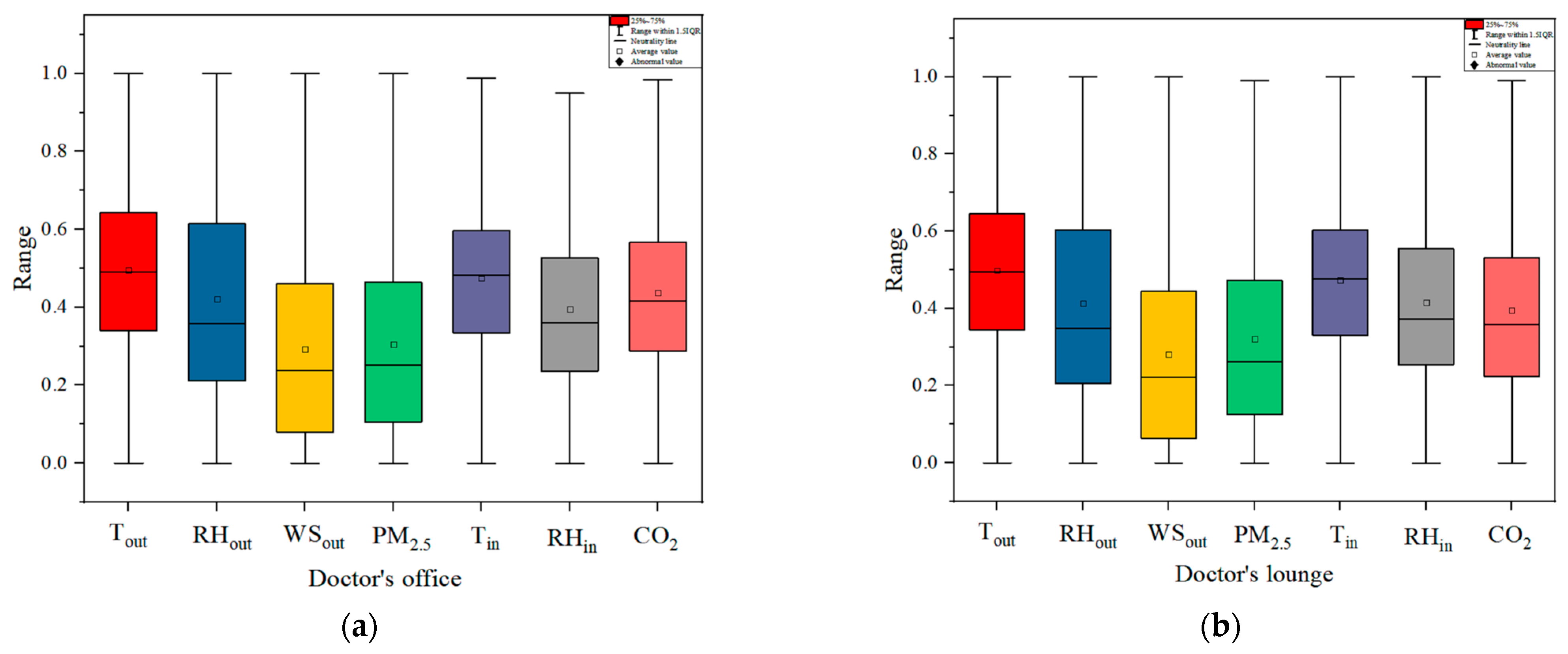
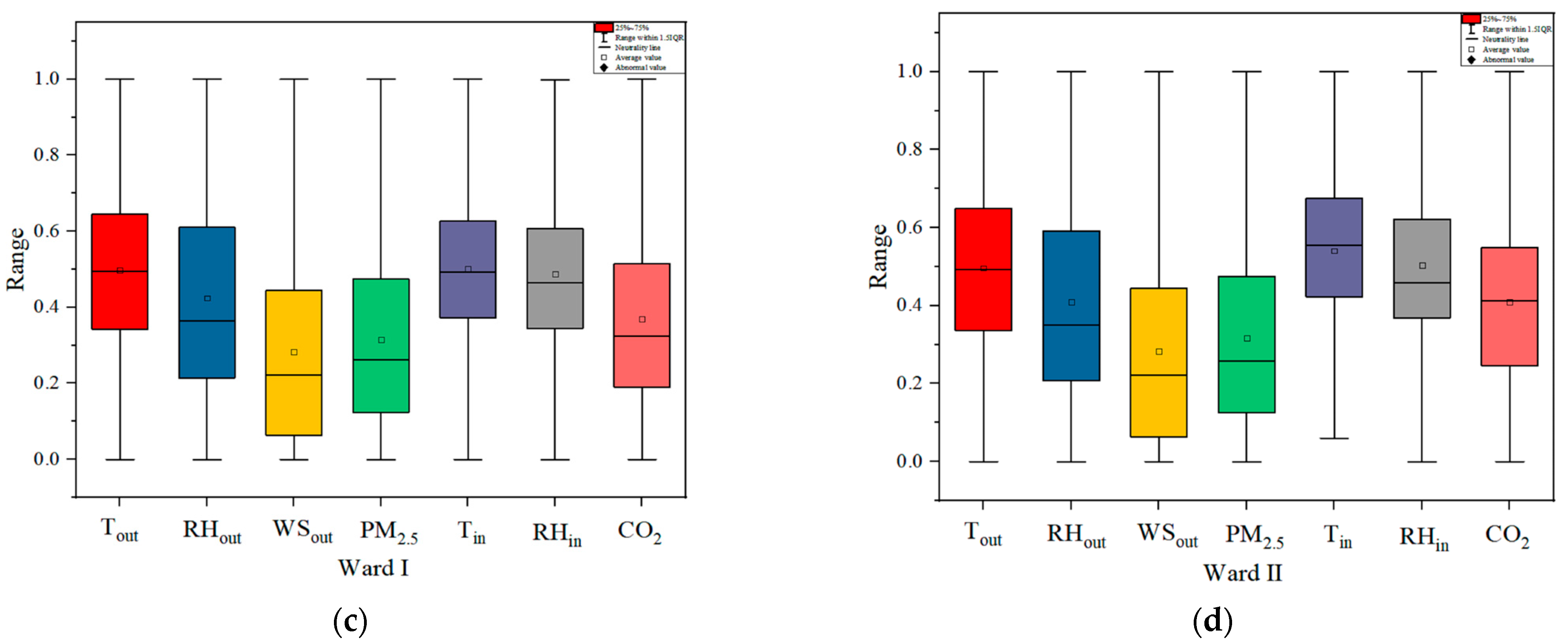
Several assumptions must be satisfied before modeling the logistic regression model [42]. First of all, it is essential to remove outliers with significant influence. If there are too many outliers, the model’s overall accuracy will be affected. The standard IQR rule was used to eliminate abnormal values [53], and the box diagram was used to test them. Figure 10 shows the filtered box diagram of each room’s data. The figure indicates that the abnormal values of all data were completely deleted.
Secondly, it determines the number of covariates in the logistic regression model. Too many covariates will lead to the over-fitting of the model. The number of covariances that the logistic regression model can accommodate was determined using the minimum number of events in the data. A rule of thumb, in this case, is taking the number of events corresponding to a covariant as 10–20. There are 9 covariates in this study, so the corresponding minimum number of events is 90. In this paper, there are more than 8000 data samples collected from all types of rooms, among which the number of window openings is the minimum number of events in this modeling, but there are also more than 1000 data points. Hence, the number of covariates in this modeling conforms to the provisions of the relevant empirical rules.
The third assumption is the independence of the error. Hence, the results of all sample groups are independent of each other (thus, there is no repeated response). The data collected in this study have time continuity, where time exists as an independent variable. Accordingly, the samples used in this paper are independent of each other and satisfied with this assumption.
The fourth assumption is that there is no multicollinearity or redundancy between independent variables. The hypothesis is tested using the variance inflation factor (VIF), and Table 5 shows the collinearity diagnosis results. The results show that the VIF is less than 10, and the variables have no collinearity [54].
The last point is that there is a linear relationship between continuous independent variables and the logitP. Because there are negative and zero values in the continuous variables collected this time, it cannot be verified by the traditional method of taking a natural logarithm [42]. In order to verify this hypothesis, this paper uses logistic regression modeling to derive the predicted value p and then calculates this value as LN(P/1 − P), which is the logitP. Thereafter, a linear model between logitP and each variable is established through linear regression, and whether there is a linear relationship between each continuous variable and logitP is judged by the model-fitting effect (R2). Table 6 shows the R2 values for the linear regression models of various rooms, and the fitting effects of the models are all above 90%. This shows that the fitting effect of the linear model is good, and the hypothesis is established.
Through the above steps, it is shown that the collected data meet the requirements of logistic regression modeling. Hence, the next modeling steps can be carried out. The outdoor wind direction and time are input into the model as classification variables, and the time is classified according to Section 3.4. The specific classification methods are shown in Table 7.
This paper uses the SPSS.26 software to establish the logistic regression model for monitoring data. Before modeling, the independent variable data must be carefully normalized and collinearity diagnosed to ensure that the data are comparable and there is no approximate linear relationship. Table 8 and Table 9 show the modeling results for the doctors’ office in addition to the doctors’ lounge and for the ward, respectively. Among them, the normalized regression coefficient B represents the influence of the independent variables on dependent variables. Sig. is the statistical value of p that determines whether the independent variable is statistically significant compared to the dependent variable. If p < 0.05, the difference is significant; otherwise, it is excluded.
The simulation results show that the indoor CO2 concentration greatly influences the window-opening behavior in the doctors’ office and lounge. Moreover, the indoor environment has a more pronounced influence on the window-opening behavior in the doctors’ office as compared to the outdoor environment. However, for the doctors’ lounge, the outdoor temperature along with the CO2 concentration have the most significant influence, followed by the indoor temperature. This shows that doctors are in different states and pay special attention to the environment. Doctors in a working state pay attention to the overall indoor environment, while doctors in a resting state pay attention to the ambient temperature.
For the wards, it can be seen from the modeling results that the environmental factors affecting the window-opening behavior in the three wards are similar. First, similarly to the doctors’ lounge, its window-opening behavior strongly correlates with the outdoor temperature, indicating that the room with the rest function pays more attention to the outdoor temperature change. Secondly, unlike the doctors’ lounge, the indoor and outdoor relative humidity strongly correlates with the wards’ window-opening behavior. Both are negatively correlated with the indoor relative humidity and positively correlated with the outdoor relative humidity. As a way to adjust the indoor environment, the window opening probability decreases with the increase in indoor relative humidity, which indicates that the personnel in the wards are more willing to keep the indoor air environment slightly humid, and the window opening probability increases when the outdoor relative humidity is high, which further proves this point. Moreover, it is worth noting that the outdoor PM2.5 concentration has a noticeable influence on the air quality. As a hospital building, it is more critical to timely adjust the window state according to the air quality change to ensure good air quality inside the building and patients’ health. However, from the modeling results, it is found that the window-opening behaviors of the five tested rooms have no strong correlation with the PM2.5 concentration, which deserves further attention.
For the two classified variables of time and wind direction, it can be seen from the results that the window-opening behavior in the doctors’ office shows different rules during four time periods. However, there is no significant difference between τ(3) and the reference time period in the doctors’ lounge, which indicates that the window opening probability changes with time similarly in the night and the afternoon periods. There is no significant difference between τ(1) and the reference time period in the four different periods of Ward Ⅰ. This shows that, in Ward Ⅰ, the window-opening behavior in the morning is similar to that in the night. The change law of the window opening probability with time can only be divided into noon, afternoon, and night. However, for Ward Ⅱ, the window opening probabilities for the four time periods vary with time. In addition, as far as the wind direction is concerned, eight wind directions have different influences on the four rooms’ types, indicating that the wind direction has different influences over the window-opening behavior due to different window orientations.
Equations (4)–(7) are the mathematical model formulas for the doctors’ office, doctors’ lounge, and the wards in this maternity hospital, respectively:
Doctors’ office:
log i t p = 2.961 T o u t 1.476 W S o u t 0.487 P M 2.5 o u t + 7.18 T i n + 4.43 R H i n 8.108 C O 2 i n + 0.6 τ ( 1 ) + 0.327 τ ( 2 ) 0.354 τ ( 3 ) 0.360 W D o u t ( 2 ) 0.391 W D o u t ( 3 ) 0.326 W D o u t ( 5 ) 0.543 W D o u t ( 6 ) 6.362
Doctors’ lounge:
log i t p = 4.729 T o u t 2.642 R H o u t 0.906 W S o u t 1.714 P M 2.5 o u t + 2.096 T i n + 1.444 R H i n 17.392 C O 2 i n + 0.747 τ ( 1 ) + 0.266 τ ( 2 ) 0.377 W D o u t ( 3 ) 0.911 W D o u t ( 4 ) 0.808 W D o u t ( 5 ) 0.883 W D o u t ( 6 ) 0.472 W D o u t ( 7 ) 2.379
Ward Ⅰ:
log i t p = 7.424 T o u t + 3.386 R H o u t 3.585 W S o u t + 1.902 T i n 5.633 R H i n 1.050 C O 2 i n 0.320 τ ( 2 ) 3.396 τ ( 3 ) 0.190 W D o u t ( 1 ) 0.419 W D o u t ( 2 ) 0.252 W D o u t ( 5 ) + 0.313 W D o u t ( 7 ) 4.062
Ward Ⅱ:
log i t p = 12.850 T o u t + 7.109 R H o u t 1.394 P M 2.5 o u t 0.804 W D o u t + 3.356 T i n 8.847 R H i n 3.929 C O 2 i n + 0.657 τ ( 1 ) + 0.428 τ ( 2 ) + 0.250 τ ( 3 ) 0.615 W D o u t ( 3 ) 0.572 W D o u t ( 4 ) 0.1005 W D o u t ( 5 ) 0.837 W D o u t ( 6 ) 3.590
where Tout is the outdoor temperature; Tin is the indoor temperature; RHin is the outdoor relative humidity; RHout is the outdoor relative humidity; CO2in is the indoor CO2 concentration; PM2.5out is the outdoor PM2.5 concentration; WSout is the outdoor wind speed; τ is time; WDout is the wind direction.

3.6. Evaluating Logistic Regression with EnergyPlus

In this section, using the Energy Management System (EMS) in EnergyPlus, the logistic regression model of each room is added to the EnergyPlus building model, and the indoor CO2 concentration is simulated by adding the software module of the dynamic window model. Figure 11 shows the software interface of each step in this simulation process.
Section 3.5 established the window-opening behavior model of each room, and then it will be necessary to establish the fixed schedule model for each room. The principle of establishing a fixed timetable is: compare the window opening probability of each hour with the daily average window opening probability of buildings, and if it is greater than the daily average window opening probability, it is regarded as a window opening within that hour; otherwise, it is set to the closed state [55]. Table 10 shows the fixed schedule of the window opening in each room.
Based on the above two methods, the CO2 concentration in each room is simulated and compared to the measured CO2 concentration, as shown in Figure 12a–e.
It can be seen that the indoor CO2 concentration simulated by the dynamic logistic regression model is closer to the measured results. On the other hand, the Pearson correlation test is used to test the correlation between the CO2 concentration simulated by the above two methods and the measured CO2 concentration. Table 11 lists the test results, where the Sig value indicates whether the correlation between two variables is significant, and the correlation indicates the strength of the correlation between both variables.
The results show that the simulation result for the indoor CO2 concentration using an embedded dynamic logistic regression model is better than that using a fixed schedule. Among them, the doctors’ office, Ward 1, and Ward 2 are more obvious, and the correlation is over 20% higher than it is with the fixed schedule. This shows that the dynamic model can accurately reproduce the behavior of indoor people to realize an accurate indoor CO2 concentration simulation and indicates the applicability of the logical regression model in actual cases.

3.7. Mutual Verification of Models

This section verifies and discusses the generalization of the logistic regression model in different buildings. Schweiker et al. [42] once suggested that when buildings have similar environments and only change their internal environment through windows, the regression parameters derived from one building can successfully simulate the window-opening behavior in another building. However, applying this model to Japanese residential buildings did not accurately predict this conclusion. Therefore, this paper further verifies this conclusion in Beijing. To further verify this finding, this study used the spring data for a school office and an infant’s family in Beijing [15,43], and the data for the doctors’ office discussed earlier for modeling and prediction. In addition, the window-opening behavior in the doctors’ office was predicted using a known window-opening behavior model of a residence in Beijing in spring [44]. Finally, the model prediction accuracy is comprehensively compared using various model evaluation indices. Table 12 provides descriptive statistics of the school office and the infant’s family data.
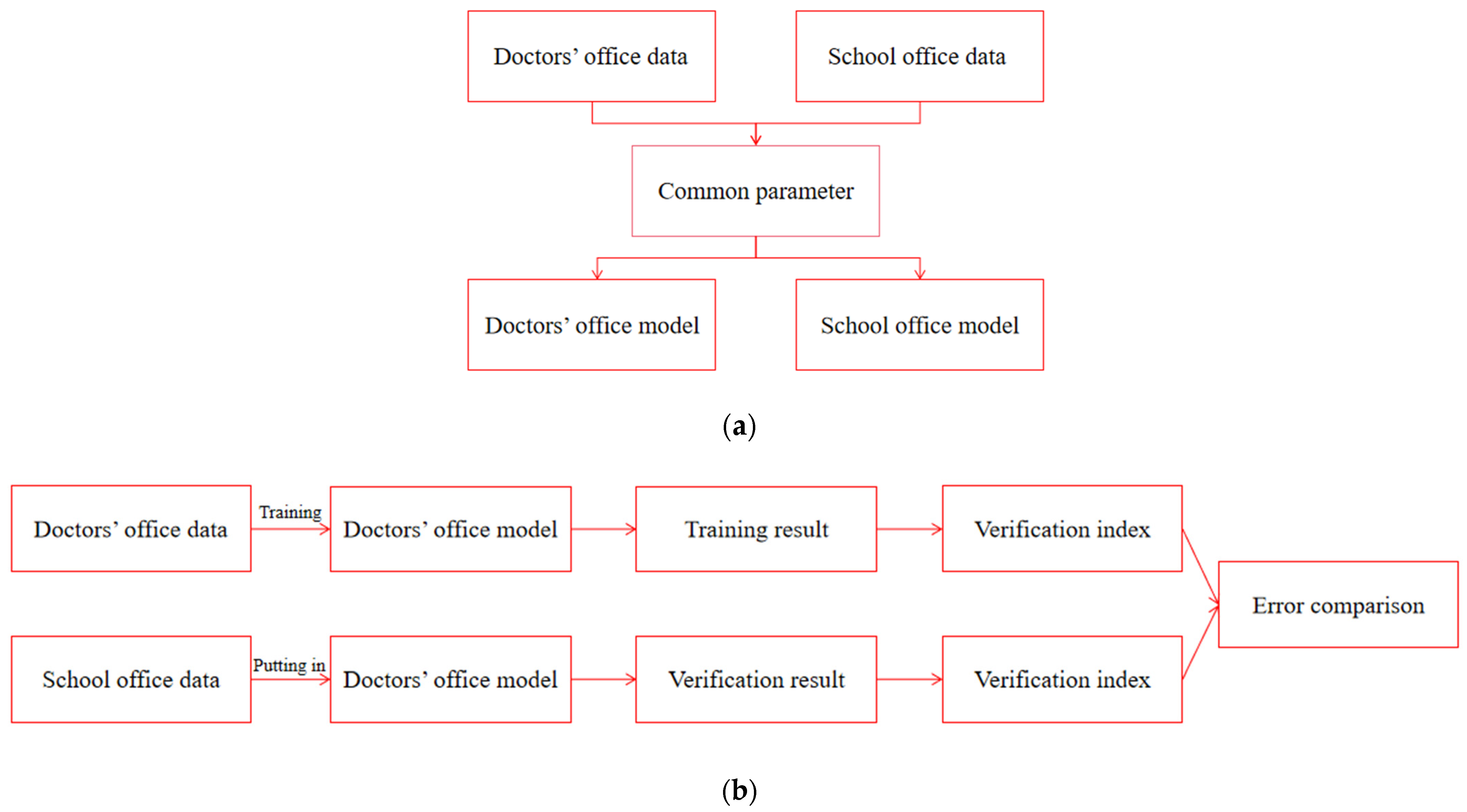
The specific verification method is as follows: firstly, three different room types (school office, infant’s family residence, and doctors’ office) are modeled. The parameter selection strategy of the model uses the same parameter of two mutually verified room types. For example, when the school office and the doctors’ office forecast each other, because the data of the school office only contains six parameters—namely indoor and outdoor temperature, outdoor humidity, outdoor PM2.5 concentration, wind direction, and wind speed—in order to ensure the fairness of the forecast, the doctors’ office model used to predict the window state of the school office should only include the six aforementioned parameters. Once the model is generated, the data of the school office will be imported into the doctors’ office’s model to obtain the school office’s predicted window state. Then, the predicted window state is compared to the actual monitored window state to determine the correctness of the model. Figure 13 shows the model verification process of the school office as an example. For the known spring residential model in Beijing, the data for the doctors’ office were directly implemented into the model to obtain the prediction results, and the results were compared with the actual statistical data of the window opening. Finally, different model evaluation indices were used to test the accuracy of the model verification, and the verification error was obtained. The specific indicators include:
1.
Window opening probability [43]
This is defined as the ratio of the window opening time to the total test time. The model prediction result is taken as the ratio of the positive sample size to the total sample size. This standard allows us to check the overall consistency of the predicted opening duration.
2.
Δ O R [55]
Δ O R is the ratio of the difference between the window opening probability predicted by the model and the actual window opening probability of the building to the actual window opening probability. According to the article’s provisions, if it falls within ±10%, the model is considered to have a good prediction effect.
3.
Number of window-opening actions [43]
The model’s predicted window opening result indicates the number of times the window state changes from closed to open. This index can compare the consistency and dynamics of window-opening behavior.
4.
Accuracy (ACC)
In the prediction results of the model, this is defined as the ratio of the correct sample size to the total sample size.
5.
F1-score [56]
When evaluating a binary classification problem, a confusion matrix is usually developed, as shown in Table 13, with columns representing the actual values and rows representing the predicted values.
The precision, calculated using Equation (8), is a positive predictive value which is defined as the proportion of the predicted positive samples in actual positive samples. As shown in Equation (9), the recall is denoted as the sensitivity and is the proportion of samples predicted to be positive that are actually positive. The F1-score, the harmonic mean of the precision and recall, as defined in Equation (10), is an indicator used in statistics to measure the accuracy of binary classification models. The higher the F1-score, the more consistent the predicted results are with the measured results.
P r e c i s i o n = T P T P + F N
R e c a l l = T P T P + F P
F 1 - s c o r e = 2 × p r e c i s i o n × r e c a l l p r e c i s i o n + r e c a l l
Table 14 shows the equations and the precision of the four models. For the school office model, because the wind direction and outdoor PM2.5 concentration do not meet the significance requirements, they are not included in this model. Table 15 shows the model prediction accuracy calculated using the above evaluation indices.
Although the building with the same environment and indoor environment is only adjusted through windows was selected, its prediction result is unsatisfactory. It can be seen from the verification results that, regardless of what kind of building model is used, the prediction results of the doctors’ office window-opening behavior have a significant error. Even for the school office buildings with similar building types, although the error of the ACC obtained is small, it is unacceptable for the indicators that describe their window-opening behavior characteristics, such as the window opening probability, window opening times, etc. This may be due to the particularity of the doctors’ office building, which leads to the significant difference between its window-opening behavior characteristics and other buildings. Therefore, its window-opening behavior model cannot predict the window-opening behavior in other building types. On the contrary, the window-opening behavior model of other building types cannot accurately reproduce the window-opening behavior in the doctors’ office. Therefore, the study of window-opening behavior in the doctors’ office still needs more accurate modeling and prediction through measured data. In addition, for other building models, it is necessary to further verify whether the accurate prediction results can be obtained under the conditions that the types of people in the rooms and the room functions are all similarly met.

4. Discussion

Each building type has its particularity, leading to the difference in the building window-opening behaviors. For example, indoor staff have commuting times to an office building, so their window-opening behavior will be affected by the indoor staff’s arrival and departure times [15,16,17,18,19]. The window-opening behavior in residential buildings will change regularly according to the household’s work and rest rules [24]. Although the window-opening behavior on the surface is influenced by time, the window-opening rules for both cases are different.
The hospital building chosen in this study varies from other building types. First of all, there are many different types of rooms in the same hospital building, including the doctors’ office, doctors’ lounge, and ward. Among them, the number of wards is the largest, which is the most important room type in hospital buildings. Therefore, in the previous research on hospital buildings, only the wards were concerned [37]. However, this paper showed that the window-opening behavior characteristics of these three types of rooms differ from each other. From the doctors’ office, even though the doctors’ office and the ordinary office are both office places, the doctors’ office does not have the same working hours as the ordinary office, so its window-opening behavior will not change regularly due to the change in the time when indoor personnel arrive and leave the office. Secondly, due to the particularity of the doctors’ profession, they pay more attention to the change in the indoor air quality, so the most significant factor affecting the window-opening behavior in the doctors’ office and doctors’ lounges is the indoor CO2 concentration, which is different from that in ordinary offices. In ordinary office buildings, the window-opening behavior is more related to the air temperature [15,16,17,18,19,20,21,22,23]. This is why, in the early window-opening behavior study, scholars only modeled the window-opening behavior according to the indoor and outdoor temperatures [45]. Furthermore, in the study of an ordinary office, indoor and outdoor environments affect window-opening behaviors. However, the window-opening behavior in hospital offices is more affected by the indoor environment. Compared to the doctors’ lounge, although the indoor staff is the same as in the doctors’ office, the window-opening behavior in the doctors’ lounge will be affected by the resting time due to the rest function. Besides the indoor air quality, the doctors’ lounge is influenced by the change in the outdoor air temperature, which is another obvious difference from the doctors’ office. For the wards, the difference with the doctor’s room is that the patient operates the window more frequently, which shows that the patient is more concerned about environmental change. Moreover, patients’ attention to the environment mainly focuses on the factors that affect the indoor thermal comfort, such as temperature and humidity, whereas their attention to air quality is weak, which is different from that of doctors’ office and doctors’ lounge.
More models that are suitable for window-opening behavior research have been developed from the research on window-opening behavior models, such as the random forest algorithm and support vector machine algorithm. They are also more accurate in predicting window-opening behavior and solving the problem of unbalanced window-opening behavior data. However, in the meantime, the model’s evaluation remains limited to the use of the model evaluation algorithm to assess the model’s prediction accuracy. Its applicability has not been tested by applying it to an actual scene. In addition, Dai et al. [41] believed that the influence of outdoor temperature, outdoor relative humidity, and other environmental parameters on window-opening behavior will lead to different window-opening habits of residents in different regions and seasons. Therefore, the model’s reliability should be carefully checked when transplanting the window state model to buildings in other seasons and regions. This paper uses a logistic regression model to simulate the buildings and study the above problems. Firstly, the logistic regression model of each room is embedded in EnergyPlus to simulate the CO2 concentration in the room and compared to the prediction result based on the fixed schedule model. The results show that the logistic regression model is superior to the fixed schedule model in terms of simulating the indoor CO2 concentration. It shows that the prediction of the window-opening behavior using this algorithm model can improve the simulation accuracy of indoor air quality in buildings as well as proves that the logistic regression model has certain applicability in actual scenes. Secondly, this study also uses a logistic regression model to verify and evaluate the doctors’ office, an infant’s family house, and a school office building. The selected buildings are all in Beijing, and the test season was spring without mechanical ventilation. The results show a significant error between the training and verification models. This finding may be due to the great difference between several types of buildings, especially the doctors’ office. This also shows that hospital buildings’ window-opening behavior differs from those of other buildings. Therefore, it is necessary to further investigate for the window-opening behavior in special buildings.

5. Limitation

In this paper, the window-opening behavior in maternity hospitals was studied, and the differences in the window-opening behaviors between the doctors’ office, doctors’ lounge, and wards were found. Additionally, two different doctor’s rooms (office and lounge) were investigated. It was found that the doctors pay different attention to the environment during office hours and rest hours, and the main factors affecting their window-opening behavior also vary. Therefore, studying the window-opening behavior in hospital buildings requires considering wards, doctors’ office, and doctors’ lounge. Generally, this study only considered the indoor and outdoor environmental factors and time but did not consider the gender, age, clothing, and other factors of indoor personnel. In the statistical process, only the opening and closing state of the window was considered, while the window’s angle and size were not considered. In addition, this study also verified the applicability of the logistic regression model in actual scenes and its generalization to other buildings. However, only the windows’ influence is considered in the actual scenario. In future research, doors, windows, air conditioners, and other structures that affect indoor air distribution can be considered comprehensively. Furthermore, due to the particularity of the doctors’ office, the logistic regression model could not achieve accurate prediction results in other buildings. Hence, in the generalization aspect, it is possible to consider the buildings with the same function and indoor personnel type for verification in the future.

6. Conclusions

In this study, the window-opening behavior in a maternity hospital in Beijing in spring is modeled and analyzed for the first time, including the influence of environmental and non-environmental factors on the window-opening behavior in the doctors’ office, doctors’ lounges, and wards. Additionally, this study also used data of different building types and data of doctors’ office in this study to build models and predict each other. The feasibility of popularizing the logistic regression model is further verified and discussed. The specific conclusions are as follows:
  • In spring, the operating frequency of ward windows is far more frequent than that of the doctor’s room, with an average of 1 to 2 times a day. The doctors’ room’s windows remain open or closed for a long time. Furthermore, in the spring, the window opening probability of all rooms increases on the day when the outdoor temperature is close to the peak of 20 °C, and after that, the phenomenon of window opening all day begins to appear.
  • According to the statistics of window opening probability changing with the time of day, it was found that the window opening probability of all rooms except the doctors’ office increased by 5% to 10% in the morning and kept decreasing after 21:00. However, as the doctors’ office is a 24 h room, its window-opening behavior did not follow this rule. Hence, the doctors’ office needs a separate analysis and modeling.
  • Doctors have different requirements for the environment under different conditions. The modeling and analysis results show that the main factors affecting the doctors’ office and the doctors’ lounge are different. The main factors affecting doctors’ office window-opening behavior are indoor environmental factors, including CO2 concentration, temperature, and relative humidity. The main factors affecting the doctors’ lounge’s window-opening behavior are indoor CO2 concentration and indoor and outdoor temperature. Therefore, two different rooms should be discussed in the hospital architecture research.
  • Outdoor temperature affects the window-opening behavior for rooms with rest functions, such as wards and doctors’ lounge. Through the modeling results, the most relevant factor to the window-opening behavior in the three wards is the outdoor temperature. Among the critical factors that affect the doctors’ lounge’s window-opening behavior, besides the indoor CO2 concentration, the most relevant one is the outdoor temperature. Therefore, when studying the window-opening behavior in buildings with rest function, it is important to pay more attention to the influence of outdoor temperature.
  • The dynamic logistic regression model can better simulate indoor air quality in actual cases. The correlation between the simulated results and the measured ones of indoor CO2 concentration by the logistic regression model in EnergyPlus software is more than 20% higher than that by the fixed timetable model.
  • Due to the room particularity, the window-opening behavior characteristics of the doctors’ office cannot be accurately predicted by the models of other buildings. Even though they are all office buildings, accurate prediction results cannot be obtained due to the differences of staff type in the room or the working hours. Therefore, the research on the doctors’ office still needs to be measured to get a more accurate prediction model. However, it is necessary to further verify whether buildings with similar room functions, types and the same personnel in the room can be mutually verified.

Author Contributions

Conceptualization, validation, investigation, resources, writing—original draft, writing—reviewing and editing, methodology, software, validation, formal analysis, Z.J.; investigation, resources, data curation, fund acquisition, project management, visualization and supervision, S.P.; formal analysis, investigation, data curation, H.Y.; formal analysis, investigation, data curation, Y.L.; resources, investigation, M.Q.; resources, data curation, S.W.; resources, data curation, L.C.; writing—reviewing and editing, supervision, Y.C. All authors have read and agreed to the published version of the manuscript.

Funding

This research was funded by the Key Laboratory for Comprehensive Energy Saving of Cold Regions Architecture of the Ministry of Education, the 13th Five-Year National Science and Technology Major Project of China (Grant Nos. 2016YFC0801706 and 2017YFC0702202), the National Natural Science Foundation of China (Grant No. 51578011), and the Technology Cooperation Center in Hebei Province (Grant No. 20594501D).

Institutional Review Board Statement

Not applicable.

Informed Consent Statement

The patient’s written informed consent has been obtained, and this article can be published.

Data Availability Statement

The data presented in this study are available on request from the corresponding author. The data are not publicly available due to the privacy policy of the studied building.

Conflicts of Interest

The authors declare no conflict of interest.

References

  1. Nicol, J.F.; Humphreys, M.A. Thermal comfort as part of a self-regulating system. Build. Res. Pr. 1973, 1, 174–179. [Google Scholar] [CrossRef]
  2. Zhong, H.-Y.; Sun, Y.; Shang, J.; Qian, F.-P.; Zhao, F.-Y.; Kikumoto, H.; Jimenez-Bescos, C.; Liu, X. Single-sided natural ventilation in buildings: A critical literature review. Build. Environ. 2022, 212, 108797. [Google Scholar] [CrossRef]
  3. Li, N.; Li, J.; Fan, R.; Jia, H. Probability of occupant operation of windows during transition seasons in office buildings. Renew. Energy 2015, 73, 84–91. [Google Scholar] [CrossRef]
  4. Smedbold, H.T.; Ahlen, C.; Unimed, S.; Nilsen, M.; Norbäck, D. εtBj⊘rn Hilt, Relationships between indoor environments and nasal inflammation in nursing personnel. Arch. Environ. Health 2002, 57, 155–161. [Google Scholar] [CrossRef] [PubMed]
  5. Gu, Y.; Cui, T.; Liu, K.; Yang, F.; Wang, S.; Song, H.; Qi, Q.; Meng, Q.; Li, Y. Study on influencing factors for occupant window opening behavior: Case study of an office building in Xi’an during the transition season. Build. Environ. 2021, 2, 107977. [Google Scholar] [CrossRef]
  6. Li, H.; Guan, Y.; Feng, G.; Huang, K. Analysis on influence of winter opening windows for natural ventilation on indoor fresh air volume in northern residential building. Procedia Eng. 2017, 205, 3323–3327. [Google Scholar] [CrossRef]
  7. Qian, H.; Li, Y.; Seto, W.H.; Ching, P.; Ching, W.H.; Sun, H.Q. Natural ventilation for reducing airborne infection in hospitals. Build. Environ. 2010, 45, 559–565. [Google Scholar] [CrossRef]
  8. Cao, Y.; Pan, S.; Liu, Y.; Yu, H.; Wang, X.; Chang, L.; Ni, M.; Liu, H. The window opening behavior of infant families: A case study during transition season in the cold region of China. Energy Build. 2022, 254, 111588. [Google Scholar] [CrossRef]
  9. Hong, T.; Yan, D.; D’Oca, S.; Chen, C.-F. Ten questions concerning occupant behavior in buildings: The big picture. Build. Environ. 2017, 114, 518–530. [Google Scholar] [CrossRef]
  10. Warren, P.R.; Parkins, L.M. Window-opening behaviour in office buildings. Build. Serv. Eng. Res. Technol. 1984, 5, 89. [Google Scholar] [CrossRef]
  11. Brundett, G.W. Ventilation: A behavioural approach. Energy Res. 1977, 1, 289–298. [Google Scholar] [CrossRef]
  12. RaJa, I.A.A.; Nicol, J.F.; McCartney, K.J. Natural ventilation buildings: Use of controls for changing indoor climate. Renew. Energy 1998, I5, 391–394. [Google Scholar] [CrossRef]
  13. Raja, I.A.; Nicol, J.F.; McCartney, K.J.; Humphreys, M.A. Thermal comfort: Use of controls in naturally ventilated buildings. Energy Build. 2001, 33, 235–244. [Google Scholar] [CrossRef]
  14. Haldi*, K.; Robinson, D. Interactions with window openings by office occupants. Build. Environ. 2009, 44, 2378–2395. [Google Scholar] [CrossRef]
  15. Pan, S.; Xiong, Y.; Han, Y.; Zhang, X.; Xia, L.; Wei, S.; Wu, J.; Han, M. A study on influential factors of occupant window opening behavior in an office building in China. Build. Environ. 2018, 133, 41–50. [Google Scholar] [CrossRef]
  16. Wei, S.; Buswell, R.; Loveday, D. Factors affecting ‘end-of-’day’ window position in a non-air-conditioned office building. Energy Build. 2013, 62, 87–96. [Google Scholar] [CrossRef]
  17. Yun, G.Y.; Steemers, K. Time-dependent occupant behaviour models of window control in summer. Building and Environ. 2008, 43, 1471–1482. [Google Scholar] [CrossRef]
  18. Zhang, Y.; Barrett, P. Factors influencing the occupants’ window opening behaviour in a naturally ventilated office building. Build. Environ. 2012, 50, 125–134. [Google Scholar] [CrossRef]
  19. Yun, G.Y.; Steemers, K. Night-time naturally ventilated offices: Statistical simulations of window-use patterns from field monitoring. Sol. Energy 2010, 84, 1216–1231. [Google Scholar] [CrossRef]
  20. Herkel, S.; Knapp, U.; Pfafferott, J. Towards a model of user behaviour regarding the manual control of windows in office buildings. Build. Environ. 2008, 43, 588–600. [Google Scholar] [CrossRef]
  21. Haldi, F.; Robinson, D. On the behaviour and adaptation of office occupants. Build. Environ. 2008, 43, 2163–2177. [Google Scholar] [CrossRef]
  22. D’Oca, S.; Hong, T. A data-mining approach to discover patterns of window opening and closing behavior in offices. Build. Environ. 2014, 82, 726–739. [Google Scholar] [CrossRef]
  23. Zhou, X.; Ren, J.; An, J.J.; Yan, D.; Shi, X.; Jin, X. Predicting open-plan office window operating behavior using the random forest algorithm. J. Build. Eng. 2021, 42, 102514. [Google Scholar] [CrossRef]
  24. Lai, D.; Jia, S.; Qi, Y.; Liu, J. Window opening behavior in Chinese residential buildings across different climate zones. Build. Environ. 2018, 142, 234–243. [Google Scholar] [CrossRef]
  25. Jeong, B.; Jeong, J.-W.; Park, J.S. Occupant behavior regarding the manual control of windows in residential buildings. Energy Build. 2016, 127, 206–216. [Google Scholar] [CrossRef]
  26. Andersen, R.V.; Toftum, J.; Andersen, K.K.; Olesen, B.W. Survey of occupant behaviour and control of indoor environment in Danish dwellings. Energy Build. 2009, 41, 11–16. [Google Scholar] [CrossRef]
  27. Du, C.; Yu, W.; Ma, Y.; Cai, Q.; Li, B.; Li, N.; Wang, W.; Yao, R. A holistic investigation into the seasonal and temporal variations of window opening behavior in residential buildings in Chongqing, China. Energy Build. 2021, 231, 110522. [Google Scholar] [CrossRef]
  28. Fabi, V.; Andersen, R.V.; Corgnati, S.; Olesen, B.W. Occupants’ window opening behaviour: A literature review of factors influencing occupant behaviour and models. Build. Environ. 2012, 58, 188–198. [Google Scholar] [CrossRef]
  29. Zhou, P.; Wang, H.; Li, F.; Dai, Y.; Huang, C. Development of window opening models for residential building in hot summer and cold winter climate zone of China. Energy Built Environ. 2021, 3, 363–372. [Google Scholar] [CrossRef]
  30. Fabi, V.; Andersen, R.K.; Corgnati, S. Verification of stochastic behavioural models of occupants’ interactions with windows in residential buildings. Build. Environ. 2015, 94, 371–383. [Google Scholar] [CrossRef]
  31. Barthelmes, V.M.; Heo, Y.; Fabi, V.; Corgnati, S.P. Exploration of the Bayesian Network framework for modelling window control behaviour. Build. Environ. 2017, 126, 318–330. [Google Scholar] [CrossRef]
  32. Mo, H.; Sun, H.; Liu, J.; Wei, S. Developing window behavior models for residential buildings using XGBoost algorithm. Energy Build. 2019, 205, 109564. [Google Scholar] [CrossRef]
  33. Jones, R.V.; Fuertes, A.; Gregori, E.; Giretti, A. Stochastic behavioural models of occupants’ main bedroom window operation for UK residential buildings. Build. Environ. 2017, 118, 144–158. [Google Scholar] [CrossRef]
  34. Hassan, A.; Zeeshan, M. Microbiological indoor air quality of hospital buildings with different ventilation systems, cleaning frequencies and occupancy levels. Atmos. Pollut. Res. 2022, 13, 101382. [Google Scholar] [CrossRef]
  35. Sham, N.M.; Ahmad, N.I.; Pahrol, M.A.; Leong, Y.-H. Fungus and mycotoxins studies in hospital environment: A scoping review. Build. Environ. 2021, 193, 107626. [Google Scholar] [CrossRef]
  36. Cheong, K.W.D.; Phua, S.Y. Development of ventilation design strategy for effective removal of pollutant in the isolation room of a hospital. Build. Environ. 2006, 41, 1161–1170. [Google Scholar] [CrossRef]
  37. Shi, Z.; Qian, H.; Zheng, X.; Lv, Z.; Li, Y.; Liu, L.; Nielsen, P.V. Seasonal variation of window opening behaviors in two naturally ventilated hospital wards. Build. Environ. 2018, 130, 85–93. [Google Scholar] [CrossRef]
  38. Hou, J.; Sun, Y.; Wang, P.; Zhang, Q.; Kong, X.; Sundell, J. Associations between ventilation and ‘children’s asthma and allergy in naturally ventilated Chinese homes. Indoor Air 2021, 31, 383–391. [Google Scholar] [CrossRef]
  39. Liu, H.; Wang, L.-L.; Zhao, S.-J.; Kwak-Kim, J.; Mor, G.; Liao, A.-H. Why are pregnant women susceptible to COVID-19? An immunological viewpoint. J. Reprod. Immunol. 2020, 139, 103122. [Google Scholar] [CrossRef]
  40. Humphreys, M.A. Classroom temperature, clothing and thermal comfort—A study of secondary school children in summertime. J. Inst. Heat. Vent. Eng. 1973, 41, 191–202. [Google Scholar]
  41. Dai, X.; Liu, J.; Zhang, X. A review of studies applying machine learning models to predict occupancy and window-opening behaviours in smart buildings. Energy Build. 2020, 223, 110159. [Google Scholar] [CrossRef]
  42. Stoltzfus, J.C. Logistic Regression: A Brief Primer. Acad. Emerg. Med. 2011, 18, 1099–1104. [Google Scholar] [CrossRef] [PubMed]
  43. Schweiker, M.; Haldi, F.; Shukuya, M.; Robinson, D. Verification of stochastic models of window opening behaviour for residential buildings. J. Build. Perform. Simul. 2012, 5, 55–74. [Google Scholar] [CrossRef]
  44. Yao, M.; Zhao, B. Factors affecting ‘occupants’ interactions with windows in residential buildings in Beijing, China. Procedia Eng. 2017, 205, 3428–3434. [Google Scholar] [CrossRef]
  45. Rijal, H.B.; Tuohy, P.; Nicol, F.; Humphreys, M.A.; Samuel, A.; Clarke, J. Development of an adaptive window-opening algorithm to predict the thermal comfort, energy use and overheating in buildings. J. Build. Perform. Simul. 2008, 1, 17–30. [Google Scholar] [CrossRef]
  46. Aqistudy. Available online: https://www.aqistudy.cn (accessed on 10 January 2023).
  47. Carlucci, S.; De Simone, M.; Firth, S.K.; Kjærgaard, M.B.; Markovic, R.; Rahaman, M.S.; Annaqeeb, M.K.; Biandrate, S.; Das, A.; Dziedzic, J.W.; et al. Modeling occupant behavior in buildings. Build. Environ. 2020, 174, 106768. [Google Scholar] [CrossRef]
  48. Stazi, F.; Naspi, F.; D’Orazio, M. Modelling window status in school classrooms. Results from a case study in Italy. Build. Environ. 2017, 111, 24–32. [Google Scholar] [CrossRef]
  49. Breiman, L. Random Forests. Mach. Lcarning 2001, 45, 5–32. [Google Scholar] [CrossRef]
  50. Li, W.; Shao, L.; Wang, W.; Li, H.; Wang, X.; Li, Y.; Li, W.; Jones, T.; Zhang, D. Air quality improvement in response to intensified control strategies in Beijing during 2013–2019. Sci. Total Environ. 2020, 744, 140776. [Google Scholar] [CrossRef]
  51. GB3095-2012; Ambient Air Quality Standards. Standardization Administration of China: Beijing, China, 2012. (In Chinese)
  52. Jin, M.; Bekiaris-Liberis, N.; Weekly, K.; Spanos, C.; Bayen, A. Sensing by proxy: Occupancy detection based on indoor CO2 concentration. UBICOMM 2015, 2015, 14. [Google Scholar]
  53. Brys, G.; Hubert, M.; Struyf, A. A Robust Measure of Skewness. J. Comput. Graph. Stat. 2004, 13, 996–1017. [Google Scholar] [CrossRef]
  54. Pisică, D.; Dammers, R.; Boersma, E.; Volovici, V. Tenets of Good Practice in Regression Analysis. A Brief Tutorial. World Neurosurg. 2022, 161, 230–239. [Google Scholar] [CrossRef] [PubMed]
  55. Chang, L.; Zhang, X.; Wang, S.; Gao, J. Control Room Contaminant Inleakage Produced by Door Opening and Closing: Dynamic Simulation and Experiments. Build. Environ. 2016, 98, 11–20. [Google Scholar] [CrossRef]
  56. Zhou, X.; Tian, S.; An, J.; Yang, J.; Zhou, Y.; Yan, D.; Wu, J.; Shi, X.; Jin, X. Comparison of different machine learning algorithms for predicting air-conditioning operating behavior in open-plan offices. Energy Build. 2021, 251, 111347. [Google Scholar] [CrossRef]
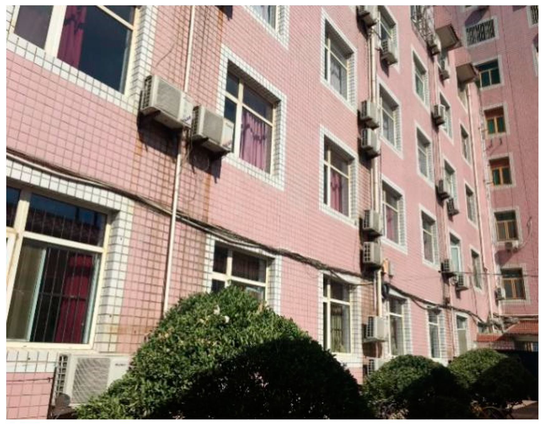
Figure 1. The exterior façade of the case study building.
Sustainability 15 08606 g001
Figure 2. The indoor air-conditioning equipment: (a) Split air conditioning system in room; (b) Radiator in the room.
Sustainability 15 08606 g002
Figure 3. Architectural layout of the case study building.
Sustainability 15 08606 g003
Figure 4. Sensors utilized to collect data in this study: (a) magnetic field strength sensor; (b) indoor temperature- and humidity-measuring device; and (c) FSR-4 portable meteorological station (temperature, humidity, wind speed, and wind direction).
Sustainability 15 08606 g004
Figure 5. Percentages and times of opened windows.
Sustainability 15 08606 g005
Figure 6. Daily window opening probability.
Sustainability 15 08606 g006
Figure 7. The relationship between the outdoor environmental factors and the window-opening behavior: (a) outdoor temperature; (b) outdoor relative humidity; (c) outdoor wind speed; (d) outdoor wind direction; and (e) outdoor PM2.5 concentration.
Sustainability 15 08606 g007aSustainability 15 08606 g007b
Figure 8. Influence of indoor environmental factors on the window-opening behavior: (a) indoor temperature; (b) indoor relative humidity; and (c) indoor CO2 concentration.
Sustainability 15 08606 g008
Figure 9. The window opening probability at different times of the day.
Sustainability 15 08606 g009
Figure 10. Outlier screening of modeling data: (a) doctors’ office; (b) doctors’ lounge; (c) Ward Ⅰ; and (d) Ward Ⅱ.
Sustainability 15 08606 g010aSustainability 15 08606 g010b
Figure 11. EMS simulation interface: (a) sensor; (b) actuator; (c) program calling manager; and (d) program.
Sustainability 15 08606 g011
Figure 12. Comparison between simulated and measured CO2 concentrations: (a) doctors’ office; (b) doctors’ lounge; (c) Ward 1; (d) Ward 2 and (e) Ward 3.
Sustainability 15 08606 g012aSustainability 15 08606 g012b
Figure 13. Model verification process: (a) modeling process; and (b) validation procedure.
Sustainability 15 08606 g013
Table 1. Experimental specifications.
Environmental
Parameters
Monitoring InstrumentsModelRangeAccuracyRecording
Interval
Indoor temperatureIndoor-monitoring
instruments
WSZY-1−20–55 °C0.1 °C10 min
Indoor relative humidity 0–100%0.1%10 min
Indoor CO2 concentrationCO2 self-recording instrumentWEZY-10–5000 ppm±75 ppm10 min
Outdoor temperatureFSR-4 portable meteorological station——−50–150 °C±0.1 °C10 min
Outdoor relative humidity0–100% RH0.1% RH10 min
Wind speed0–60 m·s–10.1 m·s–110 min
Wind direction0–360°±3°10 min
Outdoor PM2.5 concentrationMeteorological station in Tongzhou New Town [46]——————1 h
Window statusMagnetic field strength sensorCKJM-1————10 min
Note: ‘——’ means blank here.
Table 2. Descriptive statistics of the monitored environmental variables.
RoomIndexTin
(°C)
RHin
(%)
CO2in
(ppm)
Tout
(°C)
RHout
(%)
PM2.5out
(μg·m−3)
Wout
(m·s−1)
Ward 1Max28.469.1346728.39616815.4
Min18.112.2351−1.9200
Mean24.837.61209.512.136.845.83.4
Median24.936.8106711.83136.672.8
Ward 2Max30.265.7408028.39616815.4
Min1811.6351−1.9200
Mean25.137.11222.612.136.845.83.4
Median2535.7109611.83136.672.8
Ward 3Max28.574.2502628.39616815.4
Min19.814.6293−1.9200.0
Mean24.743.1145612.136.845.83.4
Median24.840.8142511.83136.72.8
Doctors’ office Max31.968.42357329815815.4
Min19.311.6305−1.91.10.00.0
Mean23.533.9721.515.240.745.72.3
Median23.631.969815.234.4371.6
Doctors’ loungeMax31.968.4497728.39616815.4
Min19.311.6352−1.9200.0
Mean23.534.1733.812.136.845.83.4
Median23.631.865511.83136.672.8
Note: Tin—indoor temperature (°C); RHin—indoor relative humidity (%); CO2in—indoor CO2 concentration (ppm); Tout—outdoor temperature (°C); RHout—outdoor relative humidity (%); PM2.5out—outdoor PM2.5 concentration (μg·m−3); Wout—outdoor wind speed (m·s−1).
Table 3. Time distribution of high CO2 indoor concentrations.
TimeOccurrence Time of CO2 High Concentration (h)
2000–2500 (ppm)2500–3000 (ppm)3000–3500 (ppm)3500–4000 (ppm)4000–4500 (ppm)4500–5000 (ppm)
0:00–1:0066.8326.81.700
1:00–2:0024.7122.12.10.30
2:00–3:0023.713.73.81.51.50
3:00–4:0024.110.89.51.10.80.7
4:00–5:0017.51410.81.301
5:00–6:0019.5174.71.30.11
6:00–7:0018.7122100.8
7:00–8:0013122100.8
8:00–9:006.15.11.30.701
9:00–10:003.13.10.300.70.3
10:00–11:002530010
11:00–12:0022.10010
12:00–13:006.12.70.10.30.70
13:00–14:005.80.50.1000
14:00–15:006.30.10000
15:00–16:005.31.30.1000
16:00–17:007.11.50000
17:00–18:0010.510000
18:00–19:008.80.80.10.30.10
19:00–20:004.50000.10.8
20:00–21:0010.820001
21:00–22:009.13.70.30.70.30
22:00–23:008.13.52.1000
23:00–24:009.83.52.1000
Table 4. Variance analysis of the results for different rooms.
RoomFDf1Df2Sig.
Doctors’ office2253.430180390.000
Doctors’ lounge620.967179460.000
Ward Ⅰ1451.652116,2780.000
Ward Ⅱ961.546171070.000
Table 5. Multicollinearity diagnosis result.
RoomOutdoor TemperatureOutdoor Relative HumidityWind SpeedOutdoor PM2.5 ConcentrationIndoor TemperatureIndoor
Relative Humidity
Indoor CO2 ConcentrationWind DirectionTime
Doctors’ office5.5477.6591.5891.7881.7127.3261.5211.0911.665
Doctors’ lounge4.2286.0841.4981.7551.6595.9261.161.081.434
Ward Ⅰ3.8014.8721.5181.6451.3733.9241.7671.0861.464
Ward Ⅱ2.7033.7641.5111.6891.262.5351.3411.0721.444
Table 6. Linear regression model fitting results.
RoomRR2Adjusted R2Std. Error of the Estimate
Doctors’ office0.9890.9790.9790.27089
Doctors’ lounge0.9920.9850.9850.19156
Ward Ⅰ0.9840.9670.9670.42048
Ward Ⅱ0.9800.9600.9600.34384
Table 7. Time classification of two types of rooms.
ClassificationWards Doctors’ Office
Τ20:00–6:00Night 00:00–6:00Early morning
τ(1)6:00–9:00Morning6:00–12:00Forenoon
τ(2)9:00–14:00Noon12:00–18:00Afternoon
τ(3)14:00–20:00Afternoon 18:00–00:00Night
Table 8. The results for the doctors’ office and lounge.
Doctors’ OfficeDoctors’ Lounge
VariableBSig. PExp(B)BSig. PExp(B)
τ 0.000 0.000
τ(1)0.6000.0001.8230.6470.0000.749
τ(2)0.3270.0121.3870.2660.0060.853
τ(3)−0.3540.0010.702−0.0940.3240.686
Wind direction 0.000 0.0000.402
Wind direction (1)0.2990.0511.348−0.2900.0510.446
Wind direction (2)−0.3600.0280.698−0.1590.2710.413
Wind direction (3)−0.3910.0070.676−0.3770.0040.624
Wind direction (4)−0.2210.0850.802−0.9110.000
Wind direction (5)−0.3260.0200.721−0.8080.0001.910
Wind direction (6)−0.5430.0040.581−0.8830.0001.304
Wind direction (7)−0.1470.3030.863−0.4720.0000.910
Outdoor temperature2.9610.00019.3254.7290.000113.193
Outdoor relative humidity0.3120.5111.367−2.6420.0000.071
Wind speed−1.4760.0000.229−0.9060.0000.404
Outdoor PM2.5 concentration−0.4870.0410.615−1.7140.0000.180
Indoor temperature7.1800.0001313.4732.9060.00018.291
Indoor relative humidity4.4430.00085.0151.4440.0014.240
Indoor CO2 concentration−8.1080.0000.000−17.3920.0000.000
Constant−6.3620.0000.002−2.3790.0000.093
Table 9. The logistic regression results of the wards.
Ward ⅠWard Ⅱ
VariableBSig. PExp(B)BSig. PExp(B)
τ 0.000 0.000
τ(1)−0.0260.7010.9740.6570.0001.928
τ(2)−0.3200.0000.7260.4280.0001.535
τ(3)−0.3960.0000.673−0.2500.0220.778
Wind direction 0.000 0.000
Wind direction (1)−0.1900.0420.827−0.2780.0770.757
Wind direction (2)−0.4190.0000.658−0.2040.1990.815
Wind direction (3)0.0520.5311.053−0.6150.0000.541
Wind direction (4)−0.1220.1070.885−0.5720.0000.564
Wind direction (5)−0.2520.0020.778−1.0050.0000.366
Wind direction (6)0.1150.2741.122−0.8370.0000.433
Wind direction (7)0.3130.0001.368−0.2030.1550.816
Outdoor temperature7.4240.0001675.60612.8500.000380,715.060
Outdoor relative humidity3.3860.00029.5417.1090.0001223.009
Wind speed−3.5850.0000.028−0.8040.0150.447
Outdoor PM2.5 concentration0.1020.4301.108−1.3940.0000.248
Indoor temperature1.9020.0006.696−3.3560.0000.035
Indoor relative humidity−5.6330.0000.004−8.8470.0000.000
Indoor CO2 concentration−1.0500.0000.350−3.9290.0000.020
Constant−4.0620.0000.017−3.5900.0000.028
Table 10. Fixed timetable for each room.
RoomTimeWindow
Doctors’ office00:00–09:000
9:00–15:001
15:00–24:000
Doctors’ lounge24:00–08:000
8:00–20:001
20:00–21:000
21:00–24:001
Ward 100:00–07:000
7:00–16:001
16:00–17:000
17:00–23:001
23:00–24:000
Ward 200:00–10:000
10:00–11:001
11:00–13:000
13:00–17:001
17:00–18:000
18:00–23:001
23:00–24:000
Ward 300:00–11:000
11:00–19:001
19:00–24:000
Table 11. Correlation comparison between simulated results and measured data of indoor CO2 concentration.
RoomLogistic RegressionFixed Schedule
CorrelationSig.CorrelationSig.
Doctors’ office−0.3110.000−0.00580.000
Doctors’ lounge−0.2720.000−0.0830.000
Ward 1−0.3180.0000.2490.000
Ward 2−0.2180.000−0.0280.029
Ward 3−0.2900.0000.0200.121
Table 12. Parameter characteristics of the school office and infant’s family residence in Beijing.
VariableMinimumMaximumAverage Value
School officeIndoor temperature (°C)17.130.724.3
Outdoor temperature (°C)8.525.3917.9
Outdoor PM2.5 concentration (µg/m3)8.0202.066.5
Outdoor relative humidity (%)9.995.640.6
Wind speed (m/s)0.04.10.91
Wind direction (°)---
Number of valid cases5943
Infant’s family residenceIndoor temperature (°C)1932.824.3
Indoor relative humidity175637.9
Indoor CO2 concentration (ppm)4003400667.0
Outdoor temperature (°C)03517.4
Outdoor relative humidity (%)119959.4
Outdoor PM2.5 concentration (µg/m3)319043.9
Wind speed (m/s)071.5
Wind direction (°)---
Number of valid cases34,241
Table 13. Confusion matrix.
Measured Result
01
Predicted result0True negative (TN)False negative (FN)
1False positive (FP) True positive (TP)
Table 14. Logistic regression models of four room types and their accuracy.
Building TypeThe Binary Logistic Regression Model
School office log i t p = 4.60 T i n + 1.00 T o u t 0.63 P M 2.5 2.95
Doctors’ officeFor school office log i t p = 6.56 T o u t + 6.96 T i n + 4.15 R H o u t 1 . 08 W S o u t 0.42 P M 2.5 + 0.29 W D o u t ( 1 ) 0.44 W D o u t ( 2 ) 0.53 W D o u t ( 3 ) 0.39 W D o u t ( 4 ) 0.61 W D o u t ( 5 ) 0.66 W D o u t ( 6 ) 9.03
For residence log i t p = 5.22 C O 2 + 7 . 12 T i n + 3 . 36 R H i n 0 . 733 P M 2.5 o u t + 4 . 47 T o u t + 1 . 74 R H o u t 1 . 19 W S o u t 7 . 612
For infant’s family residence log i t p = 4.80 C O 2 + 7.18 T i n + 3.30 R H i n 0.57 P M 2.5 + 4.46 T o u t + 1.16 R H o u t 1.00 W S o u t + 0.375 W D o u t ( 2 ) 0.34 W D o u t ( 3 ) 0.37 W D o u t ( 4 ) 0.30 W S o u t ( 6 ) 0.38 W D o u t ( 7 ) 7.52
Residence log i t p = 2.11 C O 2 + 2.096 T i n 5.277 R H i n 3.547 P M 2.5 o u t + 5.71 T o u t + 4.512 R H o u t 2.158 W S o u t 1.844
Infant’s family residence log i t p = 7.23 C O 2 0.801 T i n + 1.662 R H i n 1.84 P M 2.5 + 6.26 T o u t + 1.88 R H o u t 1.19 W S o u t + 0.264 W D o u t ( 2 ) 0.287 W D o u t ( 3 ) + 0.375 W D o u t ( 5 ) + 0.289 W D o u t ( 6 ) + 0.632 W D o u t ( 7 ) 3.35
Table 15. The models verify each other’s accuracy.
Measured DataVerification ModelWindow Opening Probability (%)OR
(%)
Window Opening TimesAcc
(%)
Precision
(%)
Recall
(%)
F1-Score
(%)
School officesDoctors’ office13.64−67.9839163.171.1622.7734.50
38.77−9.0061168.764.6258.7761.56
Error (%)25.1358.99220−5.6−6.54−36.00−27.06
Doctors’ officeSchool offices10.83−40.484678.936.5121.7527.26
8.46−53.532083.660.5928.1838.47
Error (%)2.3813.0526−4.7−24.08−6.43−11.21
Doctors’ officeResidence43.09136.7411764.329.6470.2041.68
13.39−26.413587.972.8953.6961.84
Error (%)29.69163.1582−23.6−43.25−16.50−20.16
Doctors’ officeInfant’s family residence43.00136.2958466.0531.6774.9044.51
13.67−24.908088.172.9854.8662.63
Error (%)29.34−161.19504−22.05−41.3120.04−18.12
Infant’s family residenceDoctors’ office47.20−12.7516268.879.5159.0467.77
60.6012.021577877.6484.8481.08
Error (%)−13.40%24.785−9.21.87−25.80−13.32
Disclaimer/Publisher’s Note: The statements, opinions and data contained in all publications are solely those of the individual author(s) and contributor(s) and not of MDPI and/or the editor(s). MDPI and/or the editor(s) disclaim responsibility for any injury to people or property resulting from any ideas, methods, instructions or products referred to in the content.