Abstract
There has recently been a great interest in the outdoor lighting that is energy-efficient and does not intensify a light pollution phenomenon. In architectural lighting, these demands are difficult to implement and rarely analyzed. However, it is possible to introduce and use certain parameters based on the utilization factor for the quantitative assessment of floodlighting design in terms of both light pollution and energy efficiency. This paper presents the definitions of new parameters and the results of their calculations for several typical architectural objects. Different lighting concepts were created for each object together with appropriate computer simulations. The research shows a high potential for usefulness of new parameters in the design process. The floodlighting utilization factor is characterized by relatively low values of around 35%. In addition, obtaining the recommended lighting power density value below 2.2 W/m2 does not sufficiently determine the correctness of the design implementation considering the natural environment. This determines a great potential for opportunities to improve the implemented designs and provides a basis for redefining the currently used approach in architectural lighting. In order to create high-quality, sustainable solutions, all quantitative parameters should be analyzed simultaneously in addition to the esthetic visual effect issue.
1. Introduction
In the recent years, architectural lighting designs (also known as floodlighting) have become very popular [1,2]. This trend can be seen all over the world [3,4,5]. At the beginning of the development of electric light sources, only architectural objects of the highest historical symbolic or representative rank were illuminated [6]. Some of them are still lit today. Figure 1 shows two different architectural objects where floodlighting has been implemented almost continuously for almost a century. The first of them, the Colosseum in Rome, practically has not changed at all in terms of architecture and the method of illumination. The picture of illumination of this object in 1926 can be found in book “Budapest Diszvilágitása“ written by J.B Horvath [6]. The second of them, the Saxon Palace in Poland, was destroyed during the Second World War. After the war the ruins of this building became an important memorial called the Tomb of the Unknown Soldier in Warsaw. This object is still being illuminated using up-to-date luminaires with high-efficiency electroluminescent light sources [7,8,9,10,11,12].
However, the rapid development of lighting equipment over the past few decades has resulted in architectural lighting being dedicated not only to the most important objects, but almost to any existing architectural structure, e.g., palaces, monuments, skyscrapers, bridges, churches, etc. [13]. For example, more and more designs are being implemented in Poland alone and over the past thirty years their number has increased from a dozen throughout the country to a few dozens in every larger city [14]. This is because architectural lighting creates the night-time esthetics of modern cities [3,15].

Figure 1.
Examples of architectural objects that have been almost continuously illuminated for about a century. (a) The Colosseum in Rome in 2014—photo: J. Kowalska; (b) The Saxon Palace in Warsaw in 1934 [16], (c) The Tomb of the Unknown Soldier in Warsaw in 2013—photo: K. Skarżyński.
There is also a relatively high interest in the floodlighting in the literature. Additionally, over the past twenty years, two scientific monographs, approximately 130 engineering and master’s theses and 6 doctoral dissertations on floodlighting have been prepared at the Lighting Technology Division of Warsaw University of Technology. These dissertations mainly concern modeling and floodlighting of architectural complexes [17,18] and neo-Gothic objects [19], testing the color contrast and luminance [20], as well as evaluating the floodlighting designs [21,22]. Approximately 150 commercial floodlighting designs have also been created at the authors’ research unit and a large number of them have been implemented. These architectural objects are located across Poland, Germany and the Netherlands. The number of these papers and designs provides a solid basis for conducting research and analyses in the field of floodlighting [23,24,25,26,27]. What is crucial is that all of them are based on computer visualization of lighting. Currently, floodlighting should be considered as implementing lighting designs whose main value is to obtain an esthetic effect of extraordinary beauty [28,29]. Computer software enabling the creation of such visualization is so advanced that is possible to render reality with even photorealistic accuracy [13,30,31,32,33,34]. Due to the use of computer visualization of lighting, it is possible to save time that earlier was consumed in field trials. In fact, the computer visualization method allows creation of an infinite number of floodlighting concepts, which was impossible to carry out during field trials. What is more, this relatively large number of created and implemented designs at the Lighting Technology Division of Warsaw University of Technology is only a small part compared to the multitude of architectural objects that are illuminated at night in an especially typical modern city [3,35]. More than a thousand architectural lighting installations can be found in larger cities. Each such installation has an average installed power level of approximately 4 kW. This is conditioned by the relatively high consumption of electricity, which also impacts the local economy and the functioning of the natural environment. Nowadays, there is definitely a great need to find the most ecological and high-energy-efficiency solutions [8,36,37,38,39,40]. In the context of architectural lighting, it is the right approach to find a quick, practical way to verify designs both at the design stage and after the implementation.
The main aim of this article is to present the method of quantifying an architectural lighting design based on new parameters that can be calculated and analyzed at the design level. They are mainly based on the definition of utilization factor parameters. The literature and the authors’ own observations have shown that the value of lighting efficiency in the case of architectural lighting is usually low. This paper also focuses on the results of quantitative parameter evaluation of five representative architectural objects.
2. The General Aspects of Architectural Lighting Requirements
While analyzing the night appearance of a typical city, it can be observed that in the majority of floodlighting cases, the light is directed to the object from bottom to top [23]. This means that part of a luminous flux of the luminaires may not reach the surfaces designated to be illuminated. This situation is extremely unfavorable as it impacts electrical energy losses [41,42,43,44]. A floodlighting design in which the installed power load is only a few kilowatts will not cause high losses. However, from the macro-scale point of view, a few hundred objects floodlit in an energy-inefficient way can cause relatively high and unnecessary losses of electrical energy [21]. The luminous flux not reaching the illuminated facade affects the brightening of the night sky, referred to as sky glow. It creates the light pollution phenomenon that has recently been commonly discussed in the literature in terms of its causes [45,46,47,48,49], effects [50,51,52], design recommendations [53,54,55,56], standard requirements [57,58,59], as well as measurements [60,61,62]. This phenomenon of light pollution has a harmful impact on the whole environment. Therefore, it is necessary to implement certain mechanisms and tools aimed at reducing it. The floodlighting area is extremely exposed to the intensification of this phenomenon. That is why floodlighting designs should be considered not only in terms of their visual beauty, but also in technical terms taking into account their engineering correctness. This correctness is understood as the appropriate energy efficiency and light pollution reduction in a given solution [14,21]. Until now no universal standard requirements or legal regulations have been defined for architectural lighting. In fact there is one standard related to outdoor lighting [57]. However, it does not directly relate to the issues of floodlighting. Moreover, due to the fact that there is a requirement related to the ULR (upward light ratio), it can be stated that most architectural lighting designs are prohibited completely, especially when the illumination in these designs is “from bottom to top”. It can be observed that many architectural lighting installations are designed and made in a careless manner. As a matter of fact, there are also some technical reports that refer to floodlighting referring to both energy efficiency and light pollution. They include the following documents:
- International Commission on Illumination (CIE), technical report no. 094:1993—A Guide for floodlighting [63];
- International Commission on Illumination (CIE), technical report no. 126:1997—Guidelines for minimizing sky glow [64];
- International Commission on Illumination (CIE), technical report no. 150:2017—Guide on the Limitation of the Effects of Obtrusive Light from Outdoor Lighting Installations, 2nd Edition [58];
- International Commission on Illumination (CIE), technical report no. 234:2019—A Guide to Urban Lighting Masterplanning [65];
- CIBSE (Chartered Institution of Building Services Engineers), The Society of Light and Lighting—Lighting Guide 6: The Exterior Environment [66];
- ANSI/ASHRAE/IES (American National Standards Institute/American Society of Heating, Refrigerating and Air-Conditioning Engineers Illuminating Engineering Society) Standard 90.1-2019 Energy Standard for Buildings Except Low-Rise Residential Buildings [67].
However, these give general recommendations rather than offering a full coherent design standard that is used by electrical engineers and lighting designers, as it is, for example, for road lighting [68]. These documents certainly need expanding and updating, considering current knowledge and technology, and some clarifications and better adaptation to the architectural lighting area [14]. For example, the CIE 094 and CIE 234 reports specify the average luminance parameter of the object illuminated at night. In fact, it is the only parameter that quantitatively characterizes this type of lighting. The CIE 094 report states that it can take one of the values of 4, cd/m2, 6 cd/m2, 12 cd/m2 depending on the brightness of surroundings of the illuminated object. This means the brightness of location of a given object is differentiated and the appropriate average luminance level of the object is selected in relation to it [63]. For example, an object located in a less urbanized area, e.g., in a rural area, should be characterized by a luminance of 4 cd/m2, whereas one located in the city center should be 12 cd/m2. This issue was solved in a similar way in the latest report on this field–CIE 234. However, it can be seen that the ideas from the CIE 126 and CIE 150 reports were applied. The average luminance level of illuminated objects is determined depending on the environmental zone (E1–E4) and it can take one of these recommended values: 0 cd/m2, 5 cd/m2, 10 cd/m2, 25 cd/m2. Nevertheless, a condition was added that the luminance might not exceed a certain maximum value for the specific emphasis depending on a given zone [65]. The list of the luminance requirements defined in both reports is included in Table 1.

Table 1.
Requirements of average luminance of floodlighting specified in reports CIE 094 and CIE 234 [63,65].
In the CIBSE Lighting Guide 6: The Exterior Environment publication of 2016, an algorithm for designing outdoor lighting was presented [66]. Undoubtedly, it can be useful for a lighting designer; however, it does not take into account the current possibilities of computer lighting visualization in the design process. It is very general and deals superficially with the quantitative issues of floodlighting design based on illuminance calculations instead of determining the luminance. Nevertheless, as far as floodlighting is concerned, the average luminance and the luminance distribution are important due to the light pollution phenomenon. Additionally, it should be admitted that in this publication, there are some general problems related to the low floodlighting utilization factor, which conditions the light pollution of the environment (please see Section 3.1 for the definition of floodlighting utilization factor). However, for calculations and design purposes they advise to use the assumption that its value does not exceed 30% in every case. However, this parameter ought to be as high as it is possible in the analyzed architectural lighting case. This type of approach is outdated and, for example, in many countries it was applied in the days when the software for computer aided lighting calculations had not yet been created and developed. Moreover, calculations presented in this paper will show that higher values of utilization factor in architectural lighting can be obtained.
In the case of the energy efficiency of architectural lighting, there are also standards regarding the permissible levels of lighting power density (LPD), which should be characteristic of facades of illuminated buildings. The ANSI/ASHRAE/IES document Standard 90.1-2019 Energy Standard for Buildings Except Low-Rise Residential Buildings [67] is an example of such a standard. It presents the values of lighting power density for E1–E4 individual environmental zones. In the case of architectural lighting located in urban areas (E4 zone with the high brightness), the value of the lighting power density parameter should not exceed 0.2 W/ft2, which corresponds to approximately 2.2 W/m2.
However, it is worth noting that the abovementioned technical reports do not specify in any way how to design the floodlighting of a given object so as to adapt to the average luminance level required in a given zone. The calculation method at the design level and the measurement method after implementing the designs are not described. A lack of presentation of comprehensible procedures means that probably the presented recommendations are not verified in practice. This is an unfavorable situation since the light pollution level in the environment depends on, among other things, the gained luminance levels. In the event of a shortage of the tools for their control, the implementations can be characterized by the large oversizing luminance level. Moreover, the authors are also familiar with extreme cases where the average luminance of a facade of an unilluminated object is more than 20 cd/m2 as a result of incorrect implementation of road lighting installations. Such a large oversized luminance level (simply, over-illumination) is certainly a negative aspect in any lighting applications. In this case, it should definitely be recognized as unfavorable from the point of view of light pollution and therefore some quantitative methods for its control as well as reduction should be introduced [21]. In turn, the other parameters specified in the CIE 126 and CIE 150 reports, such as upward light ratio (ULR) and upward flux ratio (UFR), determining the distribution of the luminous flux for a given luminaire or installation above the horizontal line, are in no way adapted to floodlighting needs, because, as practice shows, most luminaires used for floodlighting are directed above the skyline [58]. Nevertheless, based on the luminous flux analysis and the utilization factor parameter, it is possible to create a new, quantitative approach to floodlighting. Some useful assessment parameters (described in detail in the next chapter of this paper) can help lighting engineers to evaluate floodlighting designs in terms of light pollution and energy efficiency as well. It should be emphasized here that these new quantitative parameters cannot, however, constitute an imperative for the implementation of a given floodlighting design. In architectural lighting, the visual effect is of key importance compared to any technical and quantitative issues [14]. Nevertheless, according to the authors of this paper, it is possible (and even necessary from the point of view of the environmental issues and sustainability) to implement such floodlighting concepts that will be visually beautiful and characterized by high energy efficiency as well as minimal generation of environmental light pollution. For this purpose, the authors propose a completely new, quantitative approach to architectural lighting designs.
3. Materials and Methods
3.1. Parameters of Quantitative Assessment of Floodlighting Design-Definitions
When conducting research in the architectural lighting design field, a shortage of the tools and parameters linked to the quantitative analysis of this issue is revealed. Until now the designs and implementations of floodlighting designs have been assessed only qualitatively on the basis of a designers’ (or investor’s or heritage conservator’s) subjective vision and their sense of aesthetics. This makes the designs (usually) visually beautiful, but it is not clear if they are just so well designed when it comes to the electrical energy consumption by their lighting installation. So far the issue of energy efficiency of architectural lighting has not been analyzed due to the utilization factor or the minimizing of lighting equipment power under certain photometric assumptions. It seems to be unfavorable due to the high demand for implementation of near-zero energy solutions [37,38,69]. Moreover, the literature review shows that some countries have introduced some hard-to-achieve requirements connected with the floodlighting utilization factor (min. 75%) in order to reduce light pollution [70]. Unfortunately, a shortage of the tools and methods for controlling light pollution from the floodlighting of objects is also seen and they have to be immediately developed. For this purpose, the utilization factor, one of the basic parameters of lighting technology, can be used and it can be applied to the object of illumination as the floodlighting utilization factor [26]. Additionally, for the quantitative assessment of floodlighting design, where many luminaires of different types have been used, other parameters derived directly from the floodlighting utilization factor and based on the analysis of individual luminous fluxes are also useful. These parameters are: maximum floodlighting utilization factor, coefficient of floodlighting utilization factor and oversizing luminance. The definitions of some parameters have already been presented in the literature [26]. However, because of their specific development, they are also presented below in this paper.
The floodlighting utilization factor (1) is the ratio between the total useful luminous flux that directly reaches the designated area of the object to be floodlit and causes some specific visual effects in the form of luminance distribution and the total luminous flux of all light sources (2).
The maximum floodlighting utilization factor(3) is the ratio of the total luminous flux emitted from all luminaires used in a given solution (4) and the total luminous flux coming from all light sources (2). Its value directly gives information on the quality of lighting equipment applied to a given solution. In fact, it is the weighted arithmetic mean of light output ratios for a given project. The higher the values of light output ratios are, the higher the value of the maximum floodlighting utilization factor parameter is. Moreover, the issue of absolute photometry should be briefly discussed as the most common phenomenon for LED luminaires. It is a negative aspect because the light output ratio (LOR) enables one to obtain knowledge about energy conversion in the optical system. On this basis, it can be emphasized that manufacturers of lighting equipment face this problem because the majority of them provide the luminous efficacy of the luminaire (and not the light sources themselves).
The coefficient of floodlighting utilization factor (5) means the ratio between the gained value of the floodlighting utilization factor for a particular lighting solution and the maximum floodlighting utilization factor for a given project. However, if the proper definitions of the floodlighting utilization factor and maximum floodlighting utilization factor are carefully analyzed, it can be defined as the quotient of the useful luminous flux and the sum of the luminous fluxes of all luminaires used in a given project (5). This parameter also describes the energy potential of the design. The higher it is, the better the use of energy required for the floodlighting in the entire solution is. The range of values for this parameter is between 0 and 100%; 100% means that the total luminous flux of all luminaires used reaches the designated surfaces to be illuminated and in practice, it can be interpreted as an ideal case. The floodlighting designed in this way does not intensify light pollution since the luminous flux emitted in the upper hemisphere is only the effect of reflection of the luminous flux of luminaires from the object surface. In addition, of course, the appropriate level of average luminance of the object adjusted to the level of ambient brightness has to be obtained so that unnecessary (too large) oversizing luminance should not be created.
The oversizing luminance (6) is the value of the ratio of the gained luminance to the assumed luminance (7). This parameter is very important since it is directly connected to the energy efficiency of a given floodlighting solution. Due to specifying its value, the lighting designer can precisely determine the average luminance level the floodlighting design. This makes it possible to correct the power (luminous flux) of the luminaires used. It can be done by using an appropriate control system (dimming) or replacing the luminaires with ones of a power (luminous flux) higher/lower than the oversizing luminance gained. For example, if this parameter is 2, it means that the luminance level generated was twice as high as the assumed one. The use of luminaires with the same arrangement, luminous intensity distributions, but with twofold lower power (luminous flux) will cause the adjustment to the assumed luminance level. The oversizing luminance parameter is therefore of a great design importance. Thanks to it and any convenient lighting control tools, it is possible to adequately counteract the unwanted environmental light pollution phenomenon and have full control over the average luminance obtained in a given design.
where:
- ;
- ;
- ;
- ;
- ;
- ;
- ;
- ;
- .
3.2. Methodology for Calculating Useful Luminous Flux and Average Luminance
The main problem connected with architectural lighting design is the lack of a unified method of calculating the useful luminous flux needed to identify the floodlighting utilization factor and the average luminance (gained luminance) of the object illuminated. This is a certain inconsistency because, as shown in Section 2, architectural lighting design is projected to a given level of average luminance. However, software for computerized lighting calculations, such as DIALux or 3ds MAX, can help. Using these programs enables creation of calculation planes which will then be used for discrete calculations of the relevant photometric parameters. To do this, the analysis of a typical situation in architectural lighting, shown in Figure 2, should be performed. The luminous flux of the used luminaries can be divided into two parts: useful (useful luminous flux) and useless (the loss of luminous flux). The loss of luminous flux can be calculated by applying the cuboid method. This method can be used in any lighting simulation software. It consists of surrounding the illuminated object and the lighting equipment with computational surfaces forming a cuboid (Figure 3). Adding the luminous flux reaching each of the six cuboid faces, the loss of luminous flux is obtained (8). Bearing in mind the best computational accuracy, the side of this cuboid should be at least twice as large as the largest dimension of the analyzed object. Illuminating the faces of this solid from the inside will be a consequence of maladjustment of the luminous intensity distributions of the luminaires used (and their aiming and location) to the geometry of the floodlit object. Knowing the loss of luminous flux of a given floodlighting design, it is possible to calculate the useful luminous flux by deducting the loss of luminous flux from the total luminous flux of luminaires (9) and then all quantitative parameters presented at the beginning of this section [26]. It is worth adding that the average gained luminance can be calculated on the basis of Equation (10)—assuming the diffusion reflection phenomenon as a practical simplification. However, obtaining satisfactory computational accuracy in the case of illuminating classical architectural objects (with a small share of glass materials in the facade structure) can be achieved. However, before this is done the average weighted reflectance has to be calculated (11). Additionally, when using the cuboid method, it is essential to analyze the illuminance distributions on such sufficiently large surfaces that all luminaires used should be inside a closed surface composed of computational planes. Additionally, these planes should be characterized by an appropriate discretization which here is understood as the number of calculation points [21]. It is also worth noting that the application of this method is very useful in design practice considering the complexity of the illuminated object’s geometry. In design reality, flat facades are rare and they are usually characterized by an architectural detail. The use of this method eliminates the need to enter a large number of computational planes into the computer software, which to a great extent makes work much easier and speeds up both calculations and the entire design process.
where:
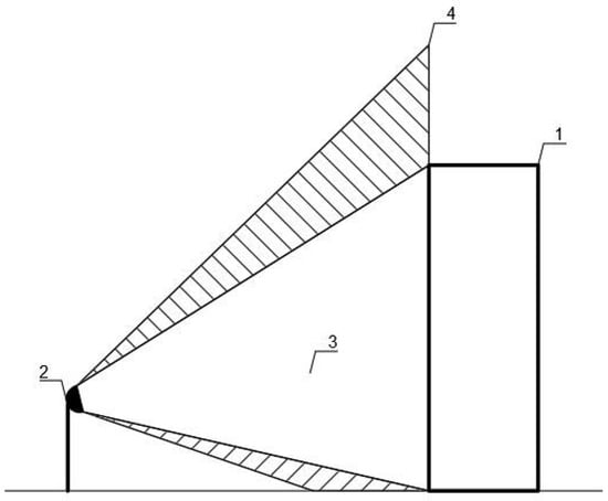
Figure 2.
Typical situation of architectural lighting: 1—architectural object (object to be floodlit), 2—luminaire, 3—useful luminous flux, 4—loss of luminous flux.
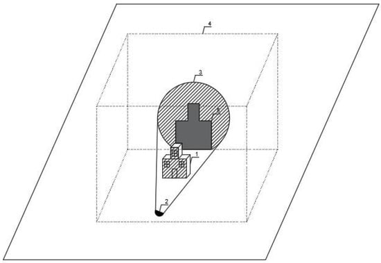
Figure 3.
Idea of calculating loss of luminous flux by the cuboid method: 1—object to be floodlit, 2—luminaire, 3—effect of loss of luminous flux, 4—closed surface surrounding object to be floodlit, 5—shadow of object.
- ;
- ;
- ;
- ;
- ;
- ;
- ;
- ;
- ;
- ;
3.3. Lighting Energy Efficiency—Installed Power and Lighting Power Density
In the case of electric lighting, the classic approach to assess the issue of energy efficiency is based on the analysis of the energy efficiency potential, i.e., parameters related to electric power of used lighting equipment. There are mainly two basic parameters: installed power and lighting power density (LPD) [71].
Installed power means the sum of the electric powers of all lighting equipment used in a given project (in a given area) (12). In general, the lower the installed capacity, the lower the electricity consumption. However, the parameters of the luminous environment must also be maintained at the appropriate level and this is the basic principle of creating energy-efficient lighting solutions [43,72].
Lighting power density means the maximum allowable value of the lighting power per illuminated area unit in relation to the appropriate classification of the type of lighting, lighting situation, environmental zone, etc. (13). As has been mentioned in the earlier part of this paper, it is recommended that the value of this parameter in the case of architectural lighting in urban areas should not exceed 2.2 W/m2 [67].
where:
- ;
- ;
- ;
- .
3.4. The Selection of Objects to Make Calculations
Floodlighting can apply to virtually all architectural objects. These objects may differ in their style of architecture. When designing the floodlighting of objects, it is necessary to consider highlighting some characteristic features of a given architectural style by using a floodlighting concept [29]. Highlighting may consist of marking the shapes of individual elements, specific rhythm of the facade, richness of decorations, etc. This means that depending on the architecture style, the appropriate way of illuminating individual surfaces should be considered by relevantly placing and aiming various types of lighting equipment (as well as selecting them in terms of their quality and photometric solidity). The authors’ experience in the field of floodlighting suggests that it would be beneficial to analyze the architectural objects that significantly differ in architectural style (geometry). For the purposes of this research, it was established that the selected objects should be a typical representation of the illuminated objects, which resulted in limiting the research to the most common architecture across Europe. As a result of this assumption, the decision on selecting the following groups of floodlit objects and their typical representatives was made (Table 2). Since the authors are Polish, objects located in Poland were chosen as the subjects of this research. It made obtaining any appropriate input data for creating the floodlighting design, such as photographic documentation or architectural plans, much easier. Therefore, for this purpose, groups of objects were defined as follows: very wide, soaring, frontage, engineering and modern. The examples of objects were determined for the appropriate group: very wide—baroque styled, soaring—Gothic and neo-Gothic styled, frontage—old tenement houses, engineering—cable-stayed bridges and high-voltage lines, modern—shopping centers and town halls. Then, as a result of the analysis of the assumptions of individual groups and their typical representatives, real objects were selected. This was the basis for the preparation of professional illumination projects in a variant approach and for the performance of its quantitative analysis.
Table 2.
List of architectural and geometric analysis results while selecting objects to carry out lighting simulations.
For all representatives of a particular group of architectural objects, the geometric models, defined materials and professional floodlighting designs (including computer visualization) were made in the Autodesk 3ds MAX software. It was agreed that 3ds Max software had sufficient calculation accuracy for the needs of simulations [32]. What is more, this software is considered by floodlighting designers as a package that enables photo realistic lighting effects to be achieved [13,30,33].
Two concepts of floodlighting were created for four out of five models. One of them presents the planar method and the other the accent method. The planar method is connected with highly uniform illumination, whereas the accent method emphasizes the architectural details. The uniformity of illumination is relatively low in this case. The proper definitions and features of the planar and accent methods can be found in [29]. The exception was an engineering structure (cable-stayed bridge), for which only one concept was made. While designing the floodlighting, no design restrictions associated with real field conditions were assumed. The most important task was to meet the floodlighting rules connected with particular floodlighting methods and to obtain a satisfactory esthetic effect, which is described in the literature [29]. For all objects and concepts, the calculations for new assessment parameters of energy efficiency and light pollution for the floodlighting design were carried out in accordance with the following assumptions:
- The cuboid method was implemented using the 3ds MAX software. It is very often used to create photorealistic visualizations of lighting, in this case the floodlighting of architectural objects. The software includes a “LightMeter” tool that allowed us to calculate the illuminance distribution on a given plane. This tool was used to create a computational cuboid surrounding individual objects.
- The condition of appropriate size/dimensions and discretization of computational surfaces was met.
- The calculations were made for the case when all the luminaires together with the object were inside the cuboid built of the computational planes.
- The calculations were made only for the direct component of lighting (without taking into account the phenomenon of interreflections).
- Lighting equipment from top quality and price manufacturers having a reputation of the highest quality of workmanship in the market was used. While choosing this equipment, attention was paid to whether the manufacturer provided all the basic data (luminous flux of light source, luminous flux of luminaire, luminaire efficiency, photometric solid) required for further calculations.
- The average reflectances should be treated as an assumption resulting from the authors’ design experience—in fact, the reflectance depends both on the type of material and the spectral power distribution (SPD) of a light source it is illuminated with.
- The average luminance levels were assumed for each analyzed object in accordance with the recommendations available in the CIE 094 report and the location of a given object: wide-stretching object—4 cd/m2, soaring object—6 cd/m2, engineering object, frontage object, modern object—12 cd/m2. Reference to the earlier CIE 094 technical report of 1993 connected with object floodlighting was made. The reason for this was in the authors’ view the increase in average luminance levels specified in the new CIE 234 report of 2019 is unfavorable from the point of view of light pollution. In general, increasing average luminance levels seems to be unnecessary and hazardous. For instance, in road lighting the highest average luminance level is 2 cd/m2, so a value from about 4–5 to about a dozen cd/m2 seems to be fine to properly distinguish the object of floodlighting from its surroundings (due to light pollution). However, the issue of the appropriate level of average luminance of the illuminated object is very complex [73]. It seems that it should also be investigated in the near future mainly in relation to environmental protection against light pollution.
- In order to assess the energy efficiency of architectural lighting, the parameters of the installed power and lighting power density were used, with the simultaneous adoption of values for these parameters from the ANSI/ASHRAE/IES Standard 90.1-2019 Energy Standard for Buildings Except Low-Rise Residential Buildings [67].
4. Results and Discussion
Figure 4, Figure 5, Figure 6, Figure 7, Figure 8, Figure 9, Figure 10, Figure 11 and Figure 12 present the results of the computer simulation of floodlighting—visualizations and luminance distributions in pseudocolor technique for the selected architectural objects. In all cases, it was noted that the designed floodlighting met the visual requirements and had satisfactory esthetic values meeting the basic floodlighting principles [29]. This means that for all objects, the illumination images obtained in the form of renderings were consistent, orderly and the lighting equipment was arranged in such a way that it was not visible to the observer. At the same time the principle of enhancing the depth and height of the object (the higher and further, the brighter) and walls perpendicular to each other have to be characterized by different luminance values. However, it should be emphasized that the issue of the reception of the floodlighting design is subjective, while the basic principles of illumination help to achieve satisfaction with the visual effects for the majority of viewers [29]. The results of the quantitative analysis are presented in Table 3 and Table 4.
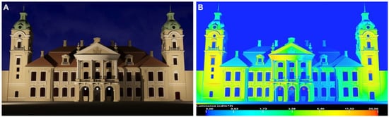
Figure 4.
Baroque palace floodlighting with the planar method: (A)—visualization, (B)—luminance distribution.
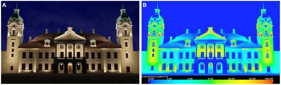
Figure 5.
Baroque palace floodlighting with the accent method: (A)—visualization, (B)—luminance distribution.
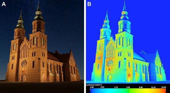
Figure 6.
Neo-Gothic church floodlighting with the planar method: (A)—visualization, (B)—luminance distribution.
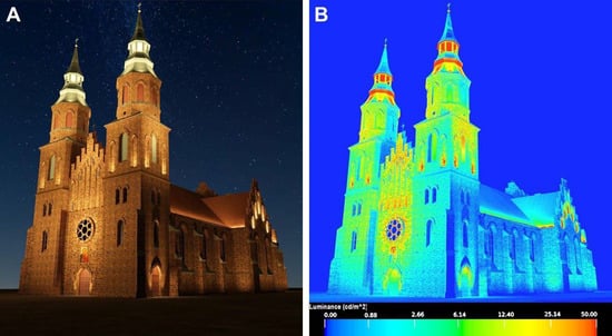
Figure 7.
Neo-Gothic church floodlighting with the accent method: (A)—visualization, (B)—luminance distribution.
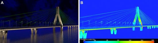
Figure 8.
Cable-stayed bridge floodlighting with the mixed method: (A)—visualization, (B)—luminance distribution.
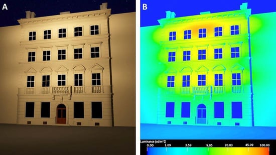
Figure 9.
Old tenement building floodlighting with the planar method: (A)—visualization, (B)—luminance distribution.
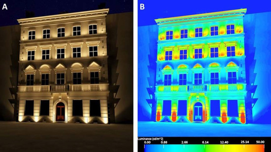
Figure 10.
Old tenement building floodlighting with the accent method: (A)—visualization, (B)—luminance distribution.
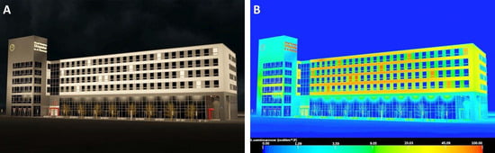
Figure 11.
Modern building floodlighting with the planar method: (A)—visualization, (B)—luminance distribution.
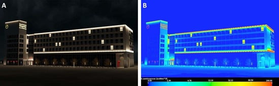
Figure 12.
Modern building floodlighting with the accent method: (A)—visualization, (B)—luminance distribution.
Table 3.
List of data used in cuboid method and results of calculations of useful luminous flux and loss of luminous flux for particular concepts of floodlighting of selected objects.
Table 4.
List of results of calculations of new parameters and luminance gained for individual concepts of floodlighting of selected objects.
Table 3 includes all the data that was used to calculate the new assessment parameters for all five objects presented in this chapter. The parameters related to the cuboid method used were also shown by specifying the side length of the cuboid that was used for the calculations as well as the mesh size of the computational grid and the number of calculation points. The side of the cuboid in individual cases as well as the discretization of the grid on the individual faces were not determined in a random way. The calculations were preceded by the analysis of these parameters and the values shown in the table are those for which the condition of “providing the sufficiently large computational planes of appropriately high discretization” was met [26]. All the luminaires applied were inside the cuboid that was used for calculations. In design and computational practice this means that there are no longer any changes in the values of individual parameters when starting with given side dimensions of the cuboid and mesh size of the computational grid. These parameters are included in Table 3. The total loss of luminous flux emitted by the applied luminaires is captured by the individual planes of the cuboid, which mainly guarantees the correctness of the method and the reliability of the results obtained. Attention is drawn to the fact that in most cases it was sufficient to create a cuboid of dimensions twice as big as the floodlit object with mesh size of 1 m. This cuboid gave a dozen or a few dozen thousand calculation points on the surface of the whole cuboid. This is an advantage because in the case of a significant increase in the number of computational points, the calculation time is significantly longer. It happens especially in the case when a very large number of luminaires are used in floodlighting design, as in the case of an engineering object—such as a cable-stayed bridge (the largest number of luminaires and the largest number of calculation points). Nevertheless, the presented calculations show that this type of analysis in floodlighting is perfectly possible. Of course, the computing ability of a given computer has also an impact; however, it is not the subject of any detailed study in this paper.
The highest value of the useful luminous flux over 1000,000 lm was obtained for a modern facility illuminated by the planar method. While the smallest value of approximately 10,000 lm was obtained for the object located in the frontage and illuminated with the accent method. These values and their difference result from the different dimensions of the objects. These examples show what differences (more than 100 times) may be in terms of the useful luminous flux requirement for various architectural objects with a different geometry and size. However, the useful luminous flux cannot be the parameter for the quantitative evaluation of the architectural lighting design because its value depends on the size of the illuminated area and, consequently, on the electric power and number of luminaires used in a given architectural lighting design.
Moreover, analyzing the obtained useful luminous flux values (Table 3), it can be seen that it is not directly related to a given floodlighting method. The general reasons for this can be a shortage of strict conditions on selecting the power and the luminous intensity distribution of luminaires with the expected value of average luminance for the floodlighting. It should be noted, however, that this inadequacy problem is only visible at the quantitative level of the floodlighting design analysis. The qualitative aspects in terms of correctness of the esthetic effect are as appropriate as possible.
Table 4 presents the calculation results of the following parameters: floodlighting utilization factor, maximum floodlighting utilization factor, coefficient of floodlighting utilization factor, gained luminance, and lighting power density. The visualization of the received data for the new parameters is presented in Figure 13 and for the lighting power density for each case in Figure 14. Table 4 also gives the value of the average reflectance for a given object, the size of the illuminated surface, the value of the average luminance for which the solution was designed. It also shows the oversizing luminance obtained as the result of dividing the value of the luminance gained (calculated) by the value of the designed luminance.
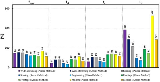
Figure 13.
Visualization of selected values of individual quantitative assessment parameters of floodlighting design obtained as a result of calculations carried out.
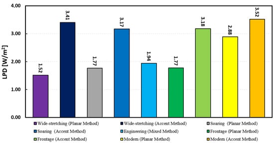
Figure 14.
Visualization of lighting power density values for particular case.
The obtained maximum floodlighting utilization factor values were around 70%. This means that about 30% of the luminous flux was lost in the optical systems of luminaires and it consequently had a negative effect on the energy efficiency of the floodlighting solution. Simultaneously analyzing this parameter indicates the need to use high-quality equipment with accurate basic quantitative data (luminous flux of light source and of luminaire, luminaire efficiency, luminous intensity distribution of luminaires) provided by its manufacturer.
The gained floodlighting utilization factor values were relatively low (around 35%). The lowest value of the floodlighting utilization factor was in the case of the cable-stayed bridge floodlighting (17%), which can be explained by the large distances from which the light came with respect to relatively small areas to be illuminated (shrouds). The highest value of the floodlighting utilization factor was obtained for floodlighting of the modern object with the planar method (56%). This means that most luminous flux from the light sources reached the surface of this object from all the discussed cases. However, it is not identical to the lowest environmental light pollution due to the nature of reflection (the directional feature dominates) and a change in value of the reflectance of glass surfaces with respect to the angle of incidence of the luminous flux directed on them. High values of this parameter (40%) were also obtained in the following cases: in the accent method for floodlighting of the wide-stretching object, the planar method for floodlighting of soaring objects as well as both methods for floodlighting of frontage objects. In addition, the generally low floodlighting utilization factor values obtained are not obvious. In all analyzed cases, the esthetic effect obtained was compliant with the rules of floodlighting art principles of floodlighting [29]. What is more, it is not stated explicitly where a given floodlighting method (planar or accent) was characterized by significantly better floodlighting utilization factor values.
While analyzing the coefficient of floodlighting utilization factor, it can be specified that its average value for all nine cases was about 50%. This means that half of the luminous flux emitted from the luminaires did not reach the surfaces designated to be floodlit and diffused in the space around the object. Both this fact and the maximum floodlighting utilization factor of 70% condition the statement that a given floodlighting design can be improved nearly twice in terms of the values of assessment parameters of floodlighting energy efficiency and light pollution.
Additionally, for all cases the average luminance value (gained luminance) and its reference to the assumed luminance level (assumed luminance) for which the design was created were calculated. So far, this has been rarely applied in practice despite the requirements set in the technical reports. The average luminance was assessed on the basis of the provisional estimation based on a visual analysis of the gained luminance distribution of a given lighting solution. As mentioned above, this method generated large errors and discrepancies in reading out the average luminance value of a given design. The obtained values as well as their reference to the designed value (oversizing luminance) show whether the average luminance level meets the assumptions. For example, the value of about 19 cd/m2 was reached for the planar method for floodlighting the wide-stretched object (Figure 4). This value is about four times higher than required (due to the location of the object in an out-of-the-way place where the level of luminance in the surroundings is very low). This means that it is possible to successfully reduce the power of the used luminaires four times, achieving a similar esthetic effect with significantly lower power consumption. Calculating the oversizing luminance also allows for a reaction when this obtained level of average luminance is lower than designed—as in cases such as engineering objects and frontage objects. In these cases, it would be necessary to look for the increase in average luminance level due to the location in a place where the surroundings are very bright: the center of a large city (frontage object) or observed from a very long distance (engineering object).
Table 4 also presents the values of the parameters of the installed power and lighting power density for particular cases. The highest value of installed power of above 19 kW was obtained for the cable-stayed bridge, and the lowest value of 0.3–0.7 kW for the facility located in the frontage. This is because these objects differ significantly in their dimensions. The area for lighting (taking into account the dimensions of the outline) in the case of the bridge was approximately 45 times larger than in the case of structures with a frontage. However, the installed power depends on the quality of the lighting equipment used, the matching of luminous intensity distribution of luminaires to the lighting task, the assumed and obtained average luminance, and mainly on the floodlighting utilization factor. In the case of the facility located in the frontage, the floodlighting utilization factor was almost 2.5 times greater than in the case of an engineering facility. Therefore, it should be concluded that in this case the architectural lighting implemented for the facility located in thefrontage was definitely more environmentally friendly than the lighting of the cable-stayed object.
Attention should also be paid to the obtained values of the lighting power density presented in Table 4 and visualized in Figure 14. Only for four of the nine analyzed cases was the value of this parameter below the standard requirement of 2.2 W/m2. These are wide, soaring objects and the frontages were illuminated with the planar method, and the cable-stayed bridge illuminated with the use of a mixed method of floodlighting. Attention is drawn to the fact that in these cases the obtained value of the floodlighting utilization factor was relatively low and in the order of 20–30%. This means that there is still a great potential for improving the energy efficiency issues for these objects. The criterion value of lighting power density was met, but a significant part of the luminous flux did not reach these objects, increasing the phenomenon of light pollution, which should definitely be eliminated. Therefore, in the case of the quantification of architectural lighting projects, it is not possible to rely solely on the criterion of lighting power density, as it may lead to incorrect conclusions that meeting the criterion value determines an environmentally friendly solution. However, all parameters should be analyzed simultaneously considering what their definitions refer to.
The results included in Table 3 and Table 4, and Figure 13 and Figure 14 do not allow us to draw any far-reaching conclusions that would combine the floodlighting method, type of object and the obtained values of assessment parameters of energy efficiency and light pollution in the object floodlighting field. For example, starting with designing the floodlighting of a given object, it is unknown whether better energy efficiency will be achieved thanks to the planar or accent method. In addition, it is not the energy efficiency that should influence a choice of floodlighting method but the esthetic vision together with all other considerations that have an impact on a selection of the floodlighting method, e.g., object observation distance, style of architecture, etc. Nevertheless, it seems that the new proposed quantitative assessment parameters can be very helpful in evaluating the engineering correctness of a given created floodlighting design. At the same time, these proposed novel parameters can certainly differentiate specific architectural lighting solutions.
5. Recommendations on Using the New Quantitative Parameters and Energy Efficiency Parameters
While analyzing the definitions of new quantitative parameters of floodlighting presented in the Section 3.1 and results of their calculations in Section 4, some general principles for their use can be specified, too. The recommendations may seem obvious after the discussion of the results in the previous section. However, in order to systematize the new approach, it is worth describing the recommendations related to the use of the new quantitative approach a little more accurately. Thus, the quality of the architectural lighting design in terms of quantity is described by the dependence (14). Firstly, the maximum floodlighting utilization factor should be as close as possible to 100%, which means that top-quality lighting equipment has been used in terms of energy conversion in the optical system. Then the floodlighting utilization factor should obtain the maximum floodlighting utilization factor, which can be checked by analyzing the coefficient of floodlighting utilization factor. As already mentioned, its value being equal to 100% will mean that the total luminous flux of all luminaires reaches only the designated surfaces to be floodlit, which is very beneficial from the perspective of light pollution. Additionally, the average gained luminance of the object should be as close as possible to the assumed value of the average value of the floodlighting design. If this happens, the oversizing luminance parameter will have a value equal to 1. This parameter shows how many times it is necessary to reduce or increase the power (luminous flux) of a given lighting system in order to adjust it to the set, assumed level of average luminance. The aim should be to achieve parameters related to energy efficiency, installed power and lighting power density close to zero. In practice, this means that these parameters should be characterized by minimum values so that it is possible to generate appropriate parameters of the luminous environment by means of an appropriate level of average luminance. Finally, it has to be stated that meeting the conditions described by Equation (14) will guarantee the implementation of the floodlighting design in a proper way in quantitative terms. That is why we should aim for the designed objects to be characterized by the desired values of quantitative parameters.
where:
- ;
- ;
- ;
- ;
- ;
- ;
- .
6. Conclusions
This paper presents a methodology for the quantitative assessment of floodlighting design (architectural lighting design). New parameters, their desired values as well as their calculation method are shown. Five typical floodlit objects that were different in geometry and architectural style were analyzed. Floodlighting was designed for each of them, with the use of the planar and accent methods. Afterwards, by the means of the presented calculation method, calculations were made for all new quantitative parameters that are used to assess the floodlighting design with respect in particular to the light pollution issue. The results of these calculations clearly show that the values of individual quantitative parameters obtained in a typical floodlighting design process are relatively low: floodlighting utilization factor of 35%, maximum floodlighting utilization factor of 68%, coefficient of floodlighting utilization factor of 50% and oversizing luminance of 1.8. The installed power parameter depends on the size of the illuminated area. As for the lighting power density value, it does not sufficiently describe the correctness of the created architectural lighting design. However, taking into account the new quantitative parameters and by analyzing all the parameters, it is possible to improve the design in terms of creating a sustainable lighting solution for a given object. This means that floodlighting designs can be improved at the design level in terms of both energy efficiency and light pollution. Finally, it has to be stated that by using these parameters it is definitely possible to quantitatively differentiate architectural lighting designs and their individual lighting solutions. This differentiation is mainly connected to the issues of energy efficiency and light pollution and can be a big advantage when it comes to creating environmentally friendly solutions.
Author Contributions
Conceptualization, K.S. and W.Ż.; methodology, K.S. and W.Ż.; validation, W.Ż.; formal analysis, K.S. and W.Ż.; investigation, K.S.; resources, K.S.; data curation, K.S.; writing—original draft preparation, K.S.; writing—review and editing, K.S.; visualization, K.S.; supervision, K.S.; project administration, K.S. All authors have read and agreed to the published version of the manuscript.
Funding
This research received no external funding.
Institutional Review Board Statement
Not applicable.
Informed Consent Statement
Not applicable.
Data Availability Statement
Data underlying the results presented in this paper are not publicly available at this time but may be obtained from the authors upon reasonable request.
Acknowledgments
Authors would like to thank the authorities of the Electrical Power Engineering Institute (Warsaw University of Technology) for financial support for proofreading and the publication fee. Moreover, authors would also like to thank the language experts from the Foreign Language Centre of Warsaw University of Technology for additional proofreading of the improved version of this paper.
Conflicts of Interest
The authors declare no conflict of interest.
References
- Mansfield, K.P. Architectural lighting design: A research review over 50 years. Light. Res. Technol. 2018, 50, 80–97. [Google Scholar] [CrossRef]
- Rea, M.S.; Figueiro, M.G. Light as a circadian stimulus for architectural lighting. Light. Res. Technol. 2018, 50, 497–510. [Google Scholar] [CrossRef]
- Talebian, K.; Riza, M. Mashhad, City of Light. Cities 2020, 101, 102674. [Google Scholar] [CrossRef]
- Chudinova, V.G.; Bokova, O.R. Possibilities of Architectural Lighting to Create New Style. In Proceedings of the IOP Conference Series: Materials Science and Engineering, Chelyabinsk, Russian, 21–22 September 2017. [Google Scholar]
- Schepetkov, N.I. Light design in London (Impressions of the specialist). Light Eng. 2008, 16, 106–116. [Google Scholar]
- Horváth, J.B. Budapest Diszvilágitása; Tungsram: Budapest, Hungary, 1989; ISBN 963-027167-2. [Google Scholar]
- Tabaka, P.; Rozga, P. Assessment of methods of marking LED sources with the power of equivalent light bulb. Bull. Pol. Acad. Sci. Tech. Sci. 2017, 65, 883–890. [Google Scholar] [CrossRef][Green Version]
- Gayral, B. LEDs for lighting: Basic physics and prospects for energy savings. C. R. Phys. 2017, 18, 453–461. [Google Scholar] [CrossRef]
- Shailesh, K.R.; Kurian, C.P.; Kini, S.G. Understanding the reliability of LED luminaires. Light. Res. Technol. 2018, 50, 1179–1197. [Google Scholar] [CrossRef]
- Czyżewski, D. Research on luminance distributions of chip-on-board light-emitting diodes. Crystals 2019, 9, 645. [Google Scholar] [CrossRef]
- Wiśniewski, A. Calculations of energy savings using lighting control systems. Bull. Pol. Acad. Sci. Tech. Sci. 2020, 68, 809–817. [Google Scholar] [CrossRef]
- Słomiński, S. Advanced modelling and luminance analysis of LED optical systems. Bull. Pol. Acad. Sci. Tech. Sci. 2019, 67, 1107–1116. [Google Scholar] [CrossRef]
- Krupiński, R. Visualization as alternative to tests on lighting under real conditions. Light Eng. 2015, 23, 22–29. [Google Scholar]
- Skarżyński, K.; Żagan, W. Opinion: Floodlighting guidelines to be updated. Light. Res. Technol. 2020, 52, 702–703. [Google Scholar] [CrossRef]
- Kowalska, J. Coloured light pollution in the urban environment. Photonics Lett. Pol. 2019, 11, 93–95. [Google Scholar] [CrossRef]
- Available online: https://polona.pl/item/warszawa-palac-saski-w-nocy,NjYyMTczNjc/0/#info:metadata/ (accessed on 24 February 2022).
- Ciupak, M. The Floodlighting of Wawel Hill in Cracow. Ph.D. Thesis, The Faculty of Electrical Engineering, Warsaw University of Technology, Warsaw, Poland, 2011. [Google Scholar]
- Krupiński, R. The Floodlighting of Architectural Complexes. Ph.D. Thesis, The Faculty of Electrical Engineering, Warsaw University of Technology, Warsaw, Poland, 2003. [Google Scholar]
- Kołodziej, M. Iluminacja Neogotyckich Obiektów Architektury Sakralnej (The Floodlighting of Neo-Gothic Sacred Architecture). Ph.D. Thesis, The Faculty of Electrical Engineering, Warsaw University of Technology, Warsaw, Poland, 2007. [Google Scholar]
- Pawlaczyk, M. Ekwiwalentność Kontrastu Barwy i Luminancji w Iluminacji (The Equivalence of the Color Contrast and the Luminance Contrast in Floodlighting). Ph.D. Thesis, The Faculty of Electrical Engineering, Warsaw University of Technology, Warsaw, Poland, 2011. [Google Scholar]
- Skarżyński, K. The Evaluation System of Floodlighting Designs in Terms of Light Pollution and Energy Efficiency. Ph.D. Thesis, The Faculty of Electrical Engineering, Warsaw University of Technology, Warsaw, Poland, 2019. (In Polish). [Google Scholar]
- Kaźmierczak, P. Badania Eksploatacyjne Stanu Oświetlenia Obiektów Iluminowanych (The Study of Utilisation in Floodlighting). Ph.D. Thesis, The Faculty of Electrical Engineering, Warsaw University of Technology, Warsaw, Poland, 2006. [Google Scholar]
- Żagan, W.; Skarżyński, K. Analysis of light pollution from floodlighting: Is there a different approach to floodlighting? Light Eng. 2017, 25, 75–82. [Google Scholar]
- Krupiński, R. Luminance distribution projection method in dynamic floodlight design for architectural features. Autom. Constr. 2020, 119, 103360. [Google Scholar] [CrossRef]
- Słomiński, S.; Krupiński, R. Luminance distribution projection method for reducing glare and solving object-floodlighting certification problems. Build. Environ. 2018, 134, 87–101. [Google Scholar] [CrossRef]
- Skarżyński, K. Methods of Calculation of Floodlighting Utilisation Factor at the Design Stage. Light Eng. 2018, 26, 144–152. [Google Scholar] [CrossRef]
- Wachta, H.; Baran, K.; Leśko, M. The meaning of qualitative reflective features of the facade in the design of illumination of architectural objects. In AIP Conference Proceedings; AIP Publishing LLC: Melville, NY, USA, 2019; Volume 2078, pp. 1–6. [Google Scholar]
- Dugar, A.M. The role of poetics in architectural lighting design. Light. Res. Technol. 2018, 50, 253–265. [Google Scholar] [CrossRef]
- Żagan, W.; Skarżyński, K. The “layered method”—A third method of floodlighting. Light. Res. Technol. 2020, 52, 641–653. [Google Scholar] [CrossRef]
- Schwarz, M.; Wonka, P. Procedural design of exterior lighting for buildings with complex constraints. ACM Trans. Graph. 2014, 33, 1–16. [Google Scholar] [CrossRef]
- Ng, E.Y.Y.; Poh, L.K.; Wei, W.; Nagakura, T. Advanced lighting simulation in architectural design in the tropics. Autom. Constr. 2001, 10, 365–379. [Google Scholar] [CrossRef]
- Reinhart, C.; Pierre-Felix, B. Experimental validation of autodesk® 3ds max® design 2009 and daysim 3.0. LEUKOS—J. Illum. Eng. Soc. N. Am. 2009, 6, 7–35. [Google Scholar] [CrossRef]
- Mahdavi, A.; Eissa, H. Subjective evaluation of architectural lighting via computationally rendered images. J. Illum. Eng. Soc. 2002, 31, 11–20. [Google Scholar] [CrossRef]
- Skarżyński, K.; Żagan, W.; Krajewski, K. Many Chips—Many Photometric and Many Chips—Many Photometric and Lighting ng Simulation Issues to Solve Simulation Issues to Solve. Energies 2021, 14, 4646. [Google Scholar] [CrossRef]
- Fichera, A.; Inturri, G.; La Greca, P.; Palermo, V. A model for mapping the energy consumption of buildings, transport and outdoor lighting of neighbourhoods. Cities 2016, 55, 49–60. [Google Scholar] [CrossRef]
- Diouf, B.; Pode, R. Development of solar home systems for home lighting for the base of the pyramid population. Sustain. Energy Technol. Assess. 2013, 3, 27–32. [Google Scholar] [CrossRef]
- Yildirim, N.; Bilir, L. Evaluation of a hybrid system for a nearly zero energy greenhouse. Energy Convers. Manag. 2017, 148, 1278–1290. [Google Scholar] [CrossRef]
- D’Agostino, D.; Parker, D. A framework for the cost-optimal design of nearly zero energy buildings (NZEBs) in representative climates across Europe. Energy 2018, 149, 814–829. [Google Scholar] [CrossRef]
- Cao, J.; Choi, C.H.; Zhao, F. Agent-based modeling of the adoption of high-efficiency lighting in the residential sector. Sustain. Energy Technol. Assess. 2017, 19, 70–78. [Google Scholar] [CrossRef]
- Sifakis, N.; Kalaitzakis, K.; Tsoutsos, T. Integrating a novel smart control system for outdoor lighting infrastructures in ports. Energy Convers. Manag. 2021, 246, 114684. [Google Scholar] [CrossRef]
- Kyba, C.C.M.; Hänel, A.; Hölker, F. Redefining efficiency for outdoor lighting. Energy Environ. Sci. 2014, 7, 1806–1809. [Google Scholar] [CrossRef]
- Al Irsyad, M.I.; Nepal, R. A survey based approach to estimating the benefits of energy efficiency improvements in street lighting systems in Indonesia. Renew. Sustain. Energy Rev. 2016, 58, 1569–1577. [Google Scholar] [CrossRef]
- Pracki, P.; Wiśniewski, A.; Czyżewski, D.; Krupiński, R.; Skarżyński, K.; Wesołowski, M.; Czaplicki, A. Strategies influencing energy efficiency of lighting solutions. Bull. Pol. Acad. Sci. Tech. Sci. 2020, 68, 711–719. [Google Scholar] [CrossRef]
- Beccali, M.; Bonomolo, M.; Lo Brano, V.; Ciulla, G.; Di Dio, V.; Massaro, F.; Favuzza, S. Energy saving and user satisfaction for a new advanced public lighting system. Energy Convers. Manag. 2019, 195, 943–957. [Google Scholar] [CrossRef]
- Jechow, A.; Kolláth, Z.; Ribas, S.J.; Spoelstra, H.; Hölker, F.; Kyba, C.C.M. Imaging and mapping the impact of clouds on skyglow with all-sky photometry. Sci. Rep. 2017, 7, 6741. [Google Scholar] [CrossRef] [PubMed]
- Witt, S.M.; Stults, S.; Rieves, E.; Emerson, K.; Mendoza, D.L. Findings from a pilot light-emitting diode (LED) bulb exchange program at a neighborhood scale. Sustainability 2019, 11, 3965. [Google Scholar] [CrossRef]
- Ouyang, J.Q.; de Jong, M.; van Grunsven, R.H.A.; Matson, K.D.; Haussmann, M.F.; Meerlo, P.; Visser, M.E.; Spoelstra, K. Restless roosts: Light pollution affects behavior, sleep, and physiology in a free-living songbird. Glob. Chang. Biol. 2017, 23, 4987–4994. [Google Scholar] [CrossRef]
- Kyba, C.C.M.; Kuester, T.; Kuechly, H.U. Changes in outdoor lighting in Germany from 2012–2016. Int. J. Sustain. Light. 2017, 19, 112. [Google Scholar] [CrossRef]
- Tabaka, P. Influence of replacement of sodium lamps in park luminaires with led sources of different closest color temperature on the effect of light pollution and energy efficiency. Energies 2021, 14, 6383. [Google Scholar] [CrossRef]
- Ngarambe, J.; Lim, H.S.; Kim, G. Light pollution: Is there an Environmental Kuznets Curve? Sustain. Cities Soc. 2018, 42, 337–343. [Google Scholar] [CrossRef]
- Gallaway, T.; Olsen, R.N.; Mitchell, D.M. The economics of global light pollution. Ecol. Econ. 2010, 69, 658–665. [Google Scholar] [CrossRef]
- Abay, K.A.; Amare, M. Night light intensity and women’s body weight: Evidence from Nigeria. Econ. Hum. Biol. 2018, 31, 238–248. [Google Scholar] [CrossRef] [PubMed]
- Doulos, L.T.; Sioutis, I.; Kontaxis, P.; Zissis, G.; Faidas, K. A decision support system for assessment of street lighting tenders based on energy performance indicators and environmental criteria: Overview, methodology and case study. Sustain. Cities Soc. 2019, 51, 101759. [Google Scholar] [CrossRef]
- Ho, C.Y.; Lin, H.T. Analysis of and control policies for light pollution from advertising signs in Taiwan. Light. Res. Technol. 2015, 47, 931–944. [Google Scholar] [CrossRef]
- Schulte-Römer, N.; Meier, J.; Dannemann, E.; Söding, M. Lighting professionals versus light pollution experts? Investigating views on an emerging environmental concern. Sustainability 2019, 11, 1696. [Google Scholar] [CrossRef]
- Pracki, P.; Skarżyński, K. A multi-criteria assessment procedure for outdoor lighting at the design stage. Sustainability 2020, 12, 1330. [Google Scholar] [CrossRef]
- EN 12464-2; Light and Lighting—Lighting of Work Places—Part 2: Outdoor Work Places. CEN (European Standard): Brussels, Belgium, 2014.
- CIE Commission Internationale de l’Eclairage. CIE 150: Guide on the Limitation of the Effects of Obtrusive Light from Outdoor Lighting Installations; CIE: Vienna, Austria, 2017. [Google Scholar]
- Gasparovsky, D. Directions of Research and Standardization in the Field of Outdoor Lighting. In Proceedings of the 7th Lighting Conference of the Visegrad Countries, Trebic, Czech Republic, 18–20 September 2018. [Google Scholar]
- Hänel, A.; Posch, T.; Ribas, S.J.; Aubé, M.; Duriscoe, D.; Jechow, A.; Kollath, Z.; Lolkema, D.E.; Moore, C.; Schmidt, N.; et al. Measuring night sky brightness: Methods and challenges. J. Quant. Spectrosc. Radiat. Transf. 2018, 205, 278–290. [Google Scholar] [CrossRef]
- Ściȩzor, T.; Kubala, M.; Kaszowski, W. Light pollution of the mountain areas in Poland. Arch. Environ. Prot. 2012, 38, 59–69. [Google Scholar] [CrossRef]
- Bertolo, A.; Binotto, R.; Ortolani, S.; Sapienza, S. Measurements of night sky brightness in the Veneto Region of Italy: Sky quality meter network results and differential photometry by digital single lens reflex. J. Imaging 2019, 5, 56. [Google Scholar] [CrossRef]
- CIE Commission Internationale de l’Eclairage. CIE 094: Guide for Floodlighting; CIE: Vienna, Austria, 1993. [Google Scholar]
- CIE Commission Internationale de l’Eclairage. CIE 126: Guidelines for Minimizing Sky Glow; CIE: Vienna, Austria, 1997. [Google Scholar]
- CIE Commission Internationale de l’Eclairage. CIE 234: A Guide for Urban Masterplanning; CIE: Vienna, Austria, 2019. [Google Scholar]
- CIBSE. CIBSE The Society of Light and Lighting—Lighting Guide 6: The Exterior Environment; CISBE: London, UK, 2016. [Google Scholar]
- ASHRAE 90.1; Energy Standard for Buildings Except Low-Rise Residential Buildings. Ashrae Standard: Atlanta, GA, USA, 2019.
- 68. EN 13201–5:2016–1-5; Road Lighitng. CEN (European Standard): Brussels, Belgium, 2016.
- Paoletti, G.; Pascuas, R.P.; Pernetti, R.; Lollini, R. Nearly Zero Energy Buildings: An overview of the main construction features across Europe. Buildings 2017, 7, 43. [Google Scholar] [CrossRef]
- Guanglei, W.; Ngarambe, J.; Kim, G. A comparative study on current outdoor lighting policies in China and Korea: A step toward a sustainable nighttime environment. Sustainability 2019, 11, 3989. [Google Scholar] [CrossRef]
- Pracki, P. A proposal to classify road lighting energy efficiency. Light. Res. Technol. 2011, 43, 271–280. [Google Scholar] [CrossRef]
- Loe, D.L. Energy efficiency in lighting—Considerations and possibilities. Light. Res. Technol. 2009, 41, 209–218. [Google Scholar] [CrossRef]
- Li, Q.F.; Yang, G.X.; Yu, L.H.; Zhang, H. A survey of the luminance distribution in the nocturnal environment in Shanghai urban areas and the control of luminance of floodlit buildings. Light. Res. Technol. 2006, 38, 185–189. [Google Scholar] [CrossRef]


Publisher’s Note: MDPI stays neutral with regard to jurisdictional claims in published maps and institutional affiliations. |
© 2022 by the authors. Licensee MDPI, Basel, Switzerland. This article is an open access article distributed under the terms and conditions of the Creative Commons Attribution (CC BY) license (https://creativecommons.org/licenses/by/4.0/).