Abstract
Land use change and demographic factors directly or indirectly affect ecosystem services value, and the analysis of ecosystem services contributes to optimization of land planning, which is essential for regional sustainable development. In this study, ArcGIS 10.2, IDRISI 17.0 Selva and MATLAB software, value coefficient method, CA-Markov prediction model and population growth model were applied to analyze the spatial and temporal changes of land use trends and ecosystem service values in Guanzhong region, and further predict the impacts of land type changes and population changes on ecosystem services in the context of urbanization. Results showed that the expansion of construction land was the most intense, and the transfer process mainly crowded out arable land; the total ecosystem services value grew spatially in a “low center-high periphery” ring with large differences at the bottom, and forest land was the most important value provider. The total ecosystem services value was estimated to decline in the future, with low-value areas spreading northward and differences in the per capita ecosystem services value increasing. This study provides a reference for optimal simulation of urban expansion and ecological conservation.
1. Introduction
Ecosystem services (ES) are the benefits that people derive directly or indirectly from ecosystems and can be categorized into four groups [1,2,3]: provisioning services (food production, raw material production, etc.), supporting services (biodiversity conservation, soil protection, etc.), regulating services (climate regulation, gas regulation, etc.) and cultural services (outdoor recreation, aesthetic landscapes, etc.). Urban ecosystems provide many benefits to residents [4,5], including the cooling effect of urban forests [6], the regulation of stormwater by urban watersheds and floodplains [7], food production of farms [8], and opportunities for recreation and scenic beauty provided by parks [9]. As ecosystem services can characterize elements and functions of an ecosystem, they have become important indicators for the study of ecological and environmental issues [10,11]. Calculating the values of ecosystem services provides a commonly-used basis for assessing the impact of changes to ecosystem services on the various components of human well-being. Presenting ecosystem service values (ESV) in monetary terms can help clarify trade-offs in decision-making processes [12], and increases understanding of the impact of economic activities on ES and the feedback effects of these changes on economic activities [13].
Although there has been progress in multiple areas of ecosystem service assessment techniques [14,15], including the development of decision tools and frameworks [16,17,18], incorporating the concept of ecosystem services in land use planning and management remains limited, at least partly because its value has not been well understood [19,20,21,22].
In Ontario, Canada, the traditional land use planning paradigm [23] has remained fundamentally unchanged since 1994. TEEB [24] echoes these statements and argues that local land use planning often lacks a full consideration of ecological well-being because the values of ecosystem services (ESV) are often identified by development sectors such as transportation, housing, water resources, economic development, tourism, and energy. Such a sectoral approach challenges the preparation of comprehensive plans that should build on linkages between the sectors [25]. In particular, de Groot [19] notes that while global and regional modeling tools can be used to assess the impacts of economic and environmental factors on natural resources, there is relatively little localized modeling and research on the interactions between land use planning and ES, as well as lack of focus on how local policy makers can actually incorporate ES considerations in land use planning, especially in the face of pressures on the quality of ES caused by a growing population [26,27].
The accelerated urbanization of the Guanzhong region has led to an increase in the area of urban built-up land, an increase in the proportion of the urban population, and an increasing pressure on the value of ES. Moreover, as this trend continues, the importance of the yield and quality of urban ESV for human well-being will continue to increase [28,29,30]. In this context, this study provides an example and reference for integrated regional ES and land use planning. Here, data, tools, and methods that are widely available and well documented are used to accomplish three objectives: (1) to quantify the extent to which land use change is subject to anthropogenic disturbance; (2) to explore the spatial and temporal variation of ESV and to elucidate its patterns of change, as well as the impact of changes in land use patterns on ecosystem services; and (3) to give some thought to how the existing land use policies and urban planning will adapt to changing conditions and learn from a better understanding the implications of ecosystem services. In the context of existing land use policies and urban planning, this study aims to explore the impacts of land use change and demographic factors on ES and provide a basis for judgment on future planning to assist policy makers in better coordinating urban development with ES.
2. Materials and Methods
2.1. Study Area
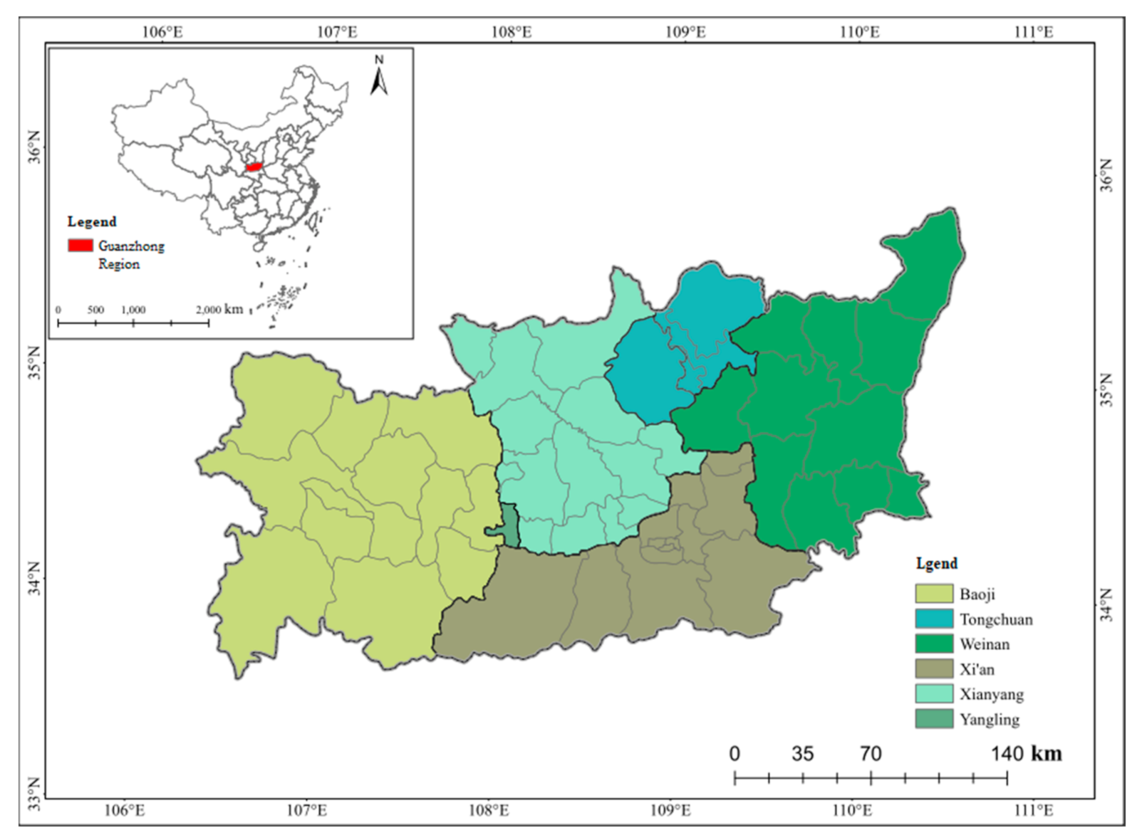
The Guanzhong region is situated within Shaanxi Province (Figure 1). To enable the merging of social statistics with data on ecosystems, county administrative boundaries were used to clarify how the data were applied our study area, which focused on Xi’an, Xianyang, (Yangling), Baoji, Tongchuan, and Weinan. The region is located between 33°35′ and 35°51′ north latitude and between 106°19′ and 110°36′ east longitude. Topographically, the Guanzhong region is a basin located between the Qinling Mountains and the Loess Plateau. LUCC, known as Land Use Cover Changes, can be classified into six categories in Guanzhong: arable land, forest land, grassland, waterbody, construction land and unused land, and these six LUCC categories are the main types of land use in this area. Here, the terrain is high in the east and low in the west. Further, the Weihe River, running through the central region, forms a large alluvial plain area (Figure 2). The Guanzhong region with semi-humid climate is a warm temperate region with four distinct seasons and a wide diversity of vegetation types and agricultural types. Economically, the region is at the heart of the economy of Northwest China and Shaanxi Province, where it plays an important role in the strategy of western development. With rapid economic development, it has also experienced a great growth in population.
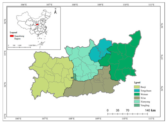
Figure 1.
Administrative map of the study area.
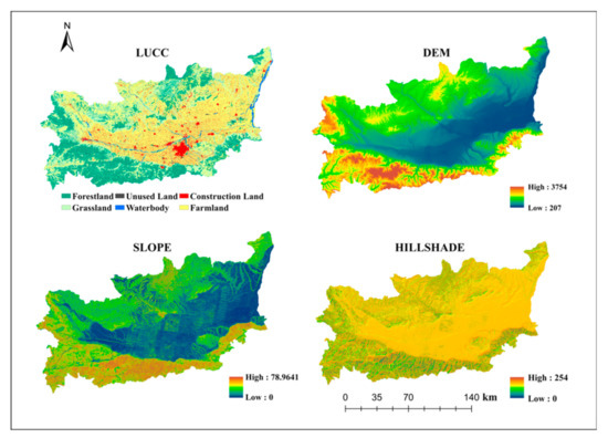
Figure 2.
Natural environment layer (LUCC is land use type (2015), DEM is digital elevation model, SLOPE is slope obtained through DEM, and HILLSHADE is mountain shading obtained through DEM).
2.2. Methods
2.2.1. LUCC Dynamics and Perturbation Analysis
Land use dynamics represent a characterization of the degree of sharpness of land class conversion over a certain period [31,32]. The land use dynamic degree quantitatively describes this rate, which is important for the comparison of regional differences and future trend predictions [33].
The single land use dynamic degree (K) [34] is calculated as follows:
where Ua and Ub refer to a certain land use type area at the start and end of the research, respectively, and T refers to the duration of the research period.
The comprehensive land use intensity index reflects the extent of human exploitation of regional land and is an essential index of the depth and breadth of regional land use. According to the comprehensive analysis method proposed by Fan [35] and other scholars, land use intensity is divided into four levels and is given a grading index, where the grading index of unused land is set at 1, that of forest land, grassland and water is set at 2, that of arable land and garden land is set at 3, and that of construction land is set at 4. The land use intensity index (LUI) can be acquired by a multiplication of the percentage of each land use type in this study area with its classification index and then weighting the sum. The formula for LUI is as follows:
where Bi is the land use intensity grading index grade of land type i and Ci is the area percentage of land type i (%).
2.2.2. Assessment of Ecosystem Service Value (ESV)
Costanza et al. [1,3] have obtained equivalent scales of service value per unit area in various ecosystems at a global scale. The equivalence factor methodology developed by Xie et al. is a unit value-based approach [36,37] and is a method widely used in China for evaluating changes in ecosystem services resulting from land use changes. In this method, each ESV is estimated as the result of a dimensionless equivalent and a unit economic value, expressed by a standard equivalence factor, and what is obtained is the value of ecosystem services generated per unit area.
According to Xie et al. [37], the ecosystem services value equivalent factor was the magnitude of the contribution of each ecological service of an ecosystem relative to the food production service of farmland, which allows the conversion of the weighting factor table into an ecosystem service value table. In the present study, the equivalence values of ES in the Guanzhong region were obtained according to the equivalence coefficient research results of Xie et al. [36,37] and Xu et al. [38].
The formula for calculating the ESV of the equivalent factor is calculated as follows:
where VCk is the ESV equivalent factor (yuan/hm2 ·a); P is the national average grain yield (yuan/kg); Qi is the average grain yield of the study area (kg/hm2); and n is the main grain type of the Guanzhong region.
where λ represents the equivalent correction factor of ESV; Ei indicates the revised ESV equivalent value of land category i (i = 1,2,…,6); Eoi denotes to the national average ecological service equivalent value of the ith category of land.
By Equations (3) and (4), the ESV per unit area in Guanzhong was acquired (Table 1).

Table 1.
ESV per unit area in the Guanzhong region yuan/(hm2·a).
Using the method described by Costanza et al. [1,3], ESV in the Guanzhong region were calculated as follows:
where ESV is the value of the ecosystem services, Si is the area of the ith type of ecosystem (hm2); Uij denotes the value coefficient of the jth ecosystem service of the ith type of ecosystem (yuan/hm2); i is the ecosystem type; j is the ecosystem service type.
2.2.3. Simulating LUCC Changes by Coupling Markov Chain and Cellular Automata
The cellular automata (CA) model is a spatial dynamic model of time, space and state discrete, and temporal causality and local spatial interaction [39]. Using the transformation rules of cell state, the spatial-temporal change process of land use and other complex systems can be simulated [40]. The model is as follows [39]:
where S(t) and S (t + 1) are the set of cellular states at times t and t + 1 respectively; F is the transition rule of the cellular state; and N is a neighborhood filter. Markov models are based on stochastic process theory [41] and were originally proposed by the former Soviet Union mathematician Andrey Markov [42]. These models can predict the future state of events by examining only current and previous data [43]. In this way, Markov models have distinct advantages in predicting future land use changes and are highly applicable for studying changes in land structure [44]. The mathematical expression is as follows:
where S(t) and S (t + 1) are the land use states at time t and time t + 1, respectively; P is the state transition probability matrix; and Pij is the probability of a transition from class i land into class j land. Here, Pij satisfies the following prerequisites:
In the field of land use simulation, Markov models are mainly about the prediction of change quantity, but they cannot indicate the spatial distribution of land use or all kinds of land change [45]. However, the CA model can predict the spatial-temporal change characteristics of all kinds of land [42], which makes up for the deficiency of the Markov model. The CA model is formulated as follows:
where Sij (t) and Sij (t + 1) are the states of the cell in row i and column j at times t and t + 1, respectively; Qij (t) is the state of the neighbors of the cell in row i and column j at time t; V is the suitability atlas; and F is the cell transformation rule.
The CA-Markov model in IDRISI 17.0 Selva software [46] was utilized to project LUCC spatial patterns of the Guanzhong region. In the CA-Markov module, an analytic hierarchy process (AHP) was applied to the determination of weights and introduced into a multi-criteria evaluation (MCE) decision to obtain the suitability map. Suitability maps were generated or provided (externally) from driver information, and each driver was considered as a real number (%).
2.2.4. Logistic Population Growth Module
The logistic model [47] was proposed by Dutch mathematician Verhulst in 1938 to study the growth pattern of biological populations in a finite space and was later used by ecologists to simulate the growth process and evolution of biological populations [48]. In this study, the logistic model is used to represent a human population growth model, where the advantage of using this model to describe the regional population growth law is that it takes into account the hindering effect of environmental conditions such as natural resources on population growth [49]. The logistic model is especially applicable to population predictions over small regions, where factor prediction is less appropriate, and where the prediction period is relatively short, which is representative of the conditions of this study. The prediction model can be written as follows:
Here, the population grows faster at the beginning of the growth period, and over time the population growth per unit of time becomes slower, until finally the population size is infinitely close to the maximum value Pm, which is reflected in the corresponding forecast target.
The criteria for fitting the logistic curve are as follows: assume that , and When t is chosen to be equally spaced, then the difference between the corresponding Pt inverse and the adjacent term can be expressed as , whose ratio of the leading term generally varies according to a fixed value, b. When using this function for the total population forecast, it is necessary to fit the historical data to derive the function and curve way for the next step of calculation. That is, by choosing three points (P0, P1, P2) equally spaced apart, and assuming that the distance between the points is n years, a system of equations can be formed as follows:
2.3. Data Resources and Processing
The resolution of LUCC, DEM, road network, population, nature reserves and illumination data are all 30 meters from the Resource and Environmental Science Data Center of the Chinese Academy of Sciences (http://www.resdc.cn/Default.aspx (accessed on 12 January 2022). The social and economic data of each county (district) from 1990 to 2020 are extracted from the “Shaanxi Regional Statistical Yearbook”, “China Counties Statistical Yearbook” and “Regional Statistical Bulletin”.
The calculation results of ESV are dimensionless processed by Max-Min normalization method. Following the guidance of Xie [36,37], the importance of each service has been considered when formulating the land ESV equivalent factor table, so the weight of each service will not be recalculated.
3. Results
3.1. Utilization and Transition of LUCC
3.1.1. LUCC Dynamic Degree
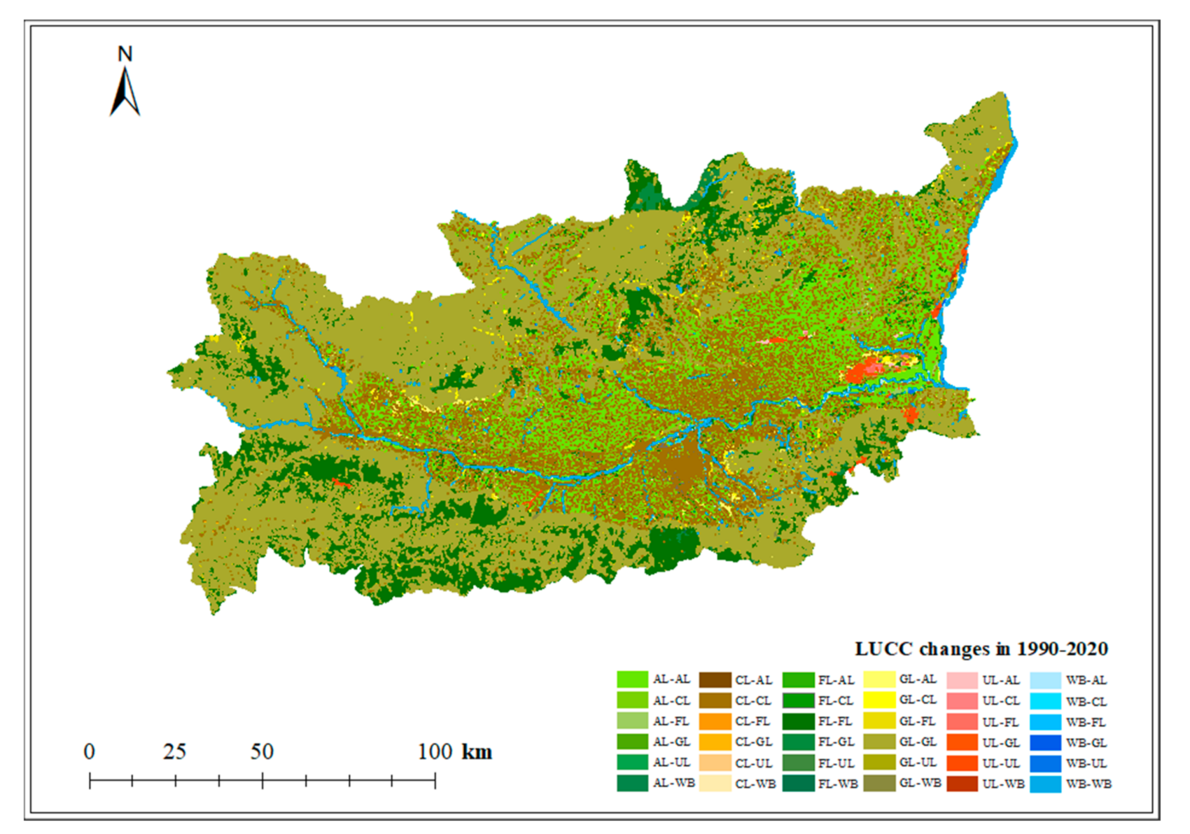
From 1990–2020, the areas of construction land, cropland, grass land and forestland experienced significant changes (Table 2 and Table 3 and Figure 3). Arable land decreased the most, reaching 169,470.28 hm2, but remained the main type of LUCC. Construction land increased the most (144,760.51 hm2) with the acceleration of urban-rural integration. The flow for construction land was the most intensive and occupied 1529.64 hm2 of arable land during the 30-year period.
Table 2.
Area changes and dynamic degree (K) of land use types in the Guanzhong region from 1990 to 2020 (%).
Table 3.
LUCC transfer matrix in the Guanzhong Region between 1990–2020 (hm2).

Figure 3.
LUCC transfer map for 1990–2020.
Approximately 1036.45 hm2 of land was returned to forests, with most expansion originating from grassland and arable land, accounting for 345.81 hm2 and 325.38 hm2 respectively. The reforestation measures were mainly distributed to the outer extension of the study area, such as the northern foot of the Qinling Mountains and the Weibei Plain. Additionally, about 35.04 hm2 of forest land expansion originated from the reforestation of unused land.
For the K-values, the most significant change among all LUCCs was in construction land (increasing by 144,760.51 hm2) with a dynamic degree of 2.25%; while the dynamic situation of conversion of forest land and grassland remains solid and steady. Since 1990, the LUCC in the Guanzhong region has been affected by both natural factors and anthropogenic development, as well as construction activities to varying degrees, including the expansion of watersheds and improvement in the protection of regional water resources.
3.1.2. Land Use Intensity Composite Index
Following the specification of Equation (2), the comprehensive index of land use intensity in the years 1990, 2005 and 2020 were obtained (Table 4). Here it can be seen that the proportion of agricultural land in the region continued to decrease between 1990 and 2020, while the area of forest land, grassland and water, which accounted for a larger proportion, continued to increase, resulting in an increasing trend of LUI in the study area from 253.63% in 1990 to 255.86% in 2020. LUI indicates human labor and capital inputs to land, i.e., higher LUI values imply more intensive land use practices, which are associated with human interference with ecosystems. In practical terms, the above trend of decreasing and then increasing LUI is also consistent with the policy of “returning farmland to forest” implemented in China in the 1990s, which led to a more active and rational development of land use resources, as well as the accelerated urbanization process of the early 21st century, which led to the intensification of land use development and human interference.
Table 4.
Comprehensive index of land use intensity in the Guanzhong region in 1990–2020 (%).
3.2. Spatial and Temporal Patterns of ESV
3.2.1. Spatial Differentiations
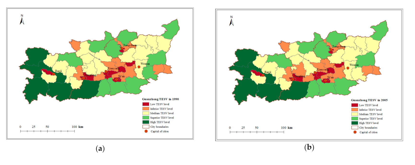
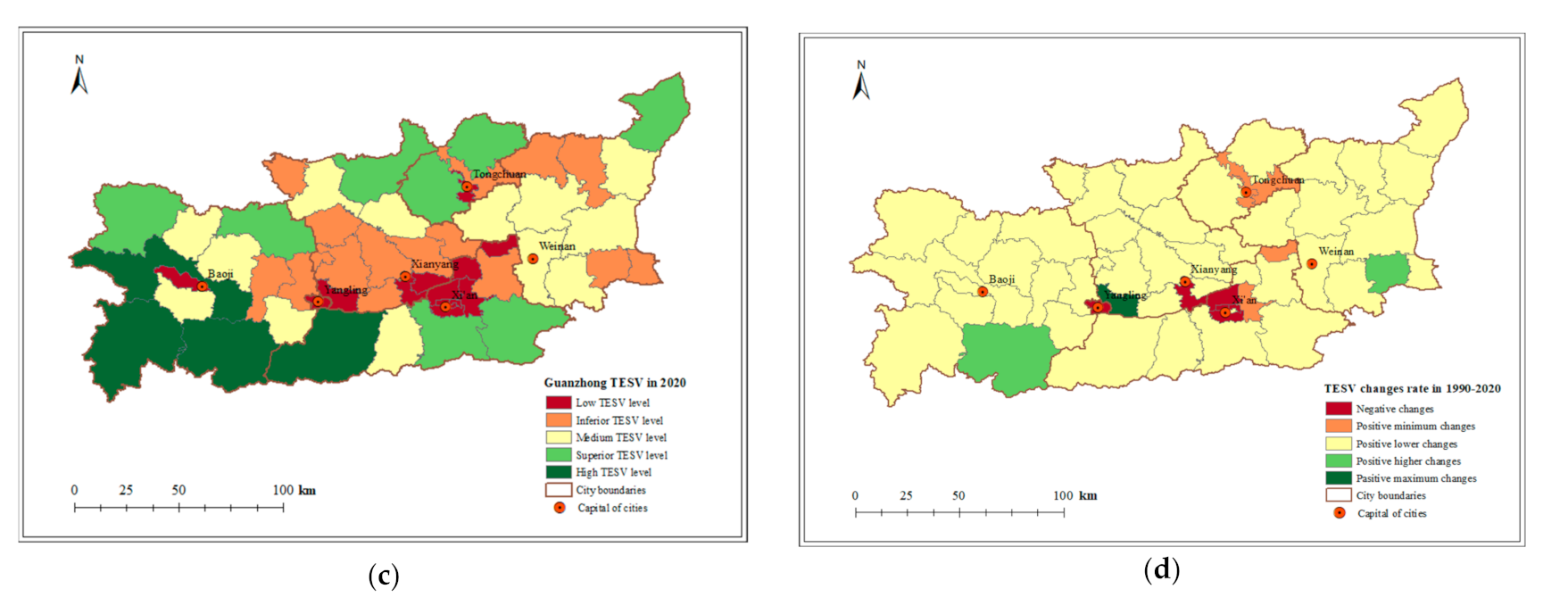
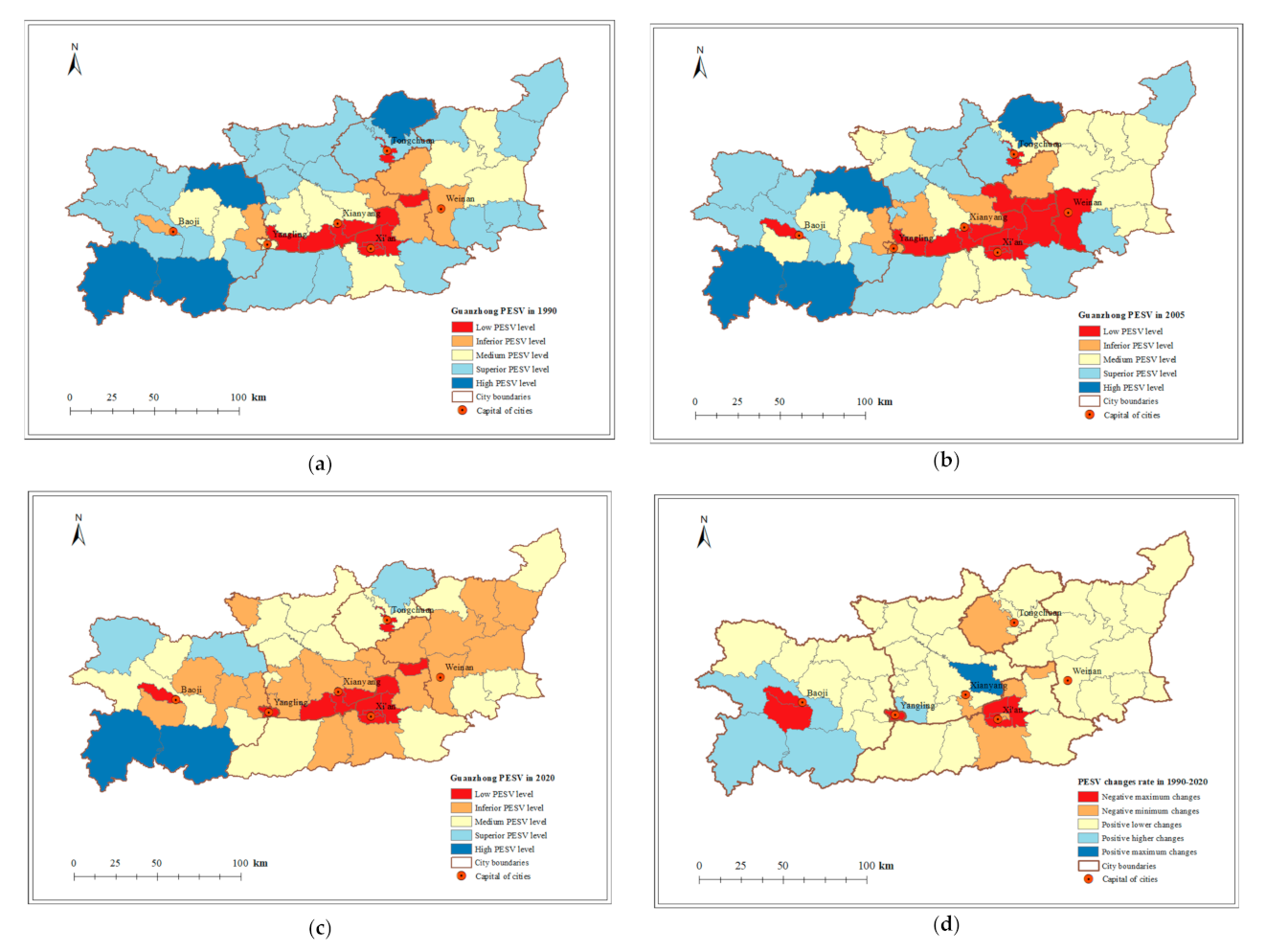
According to the calculation of Natural Jenks using ArcGIS 10.2 software, the total ESV (TESV) was classified into five classes (Figure 4). The spatial pattern of TESV in each administrative region maintained an increasing “center-periphery” circular distribution from low to high during the 30-year period (Figure 4a–d). Spatially, the TESV in the periphery was high in the west and low in the east. Xi’an City and Yangling Development Zone exhibited a negative variation, while the rest displayed positive variations.
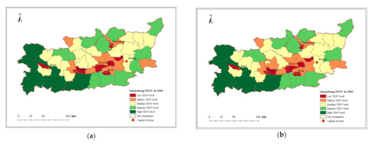

Figure 4.
TESV distribution and changes from (a) to (d).
As urban areas continue to expand, a greater proportion of the population lives in these areas and the importance of ESV for human well-being increases [28,29]. Previous studies have indicated [27,50,51] that among the many factors affecting changes in ESV, the influence of demographic factors is prominent.
To further explore the influence of demographic factors on the distribution of ESV, the spatial variation of per capita ESV (PESV) was calculated (Figure 5a–d). The results suggest that the PESV also displayed spatial variation characteristics centered on Xi’an, maintaining a progression from low to high from the interior to the periphery (Figure 4), which is in accordance with the distribution of the TESV. Among five cities, Baoji maintained the highest PESV, while Xi’an maintained the lowest. Moreover, Baoji exhibited the largest proportion of positive PESV change, while Xi’an displayed more negative PESV changes, which were mainly from the main urban area.

Figure 5.
PESV distribution and changes from (a) to (d).
3.2.2. Temporal Variations
Total ESV includes four service types: regulation services, support services, supply services and cultural services. The total ESV increased from 47,650.9 × CNY 106 to 58,852.14 × CNY 106 during the period of 1990–2020 (Table 5), during which the regulating services consistently maintained the largest contribution (51.34–51.36%).
Table 5.
Changes in primary classification of ESVs between 1990–2020.
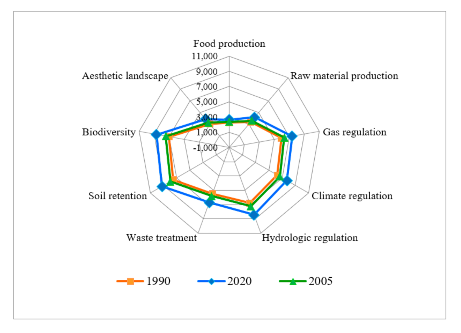
Dividing the four service types into secondary subdivisions, ESV changes are shown in Figure 4. Overall, hydrological regulation, biodiversity and soil conservation were the main ESV types among all ESVs. The ESV of soil conservation increased from 7521.43 × CNY 106 in 1990 to 9221.8 × CNY 106 in 2020 and reached the highest value; while the ESV of food production was always lower than the other ESV categories, maintaining a range of 2246.68 × CNY 106– to 2664.58 × CNY 106.
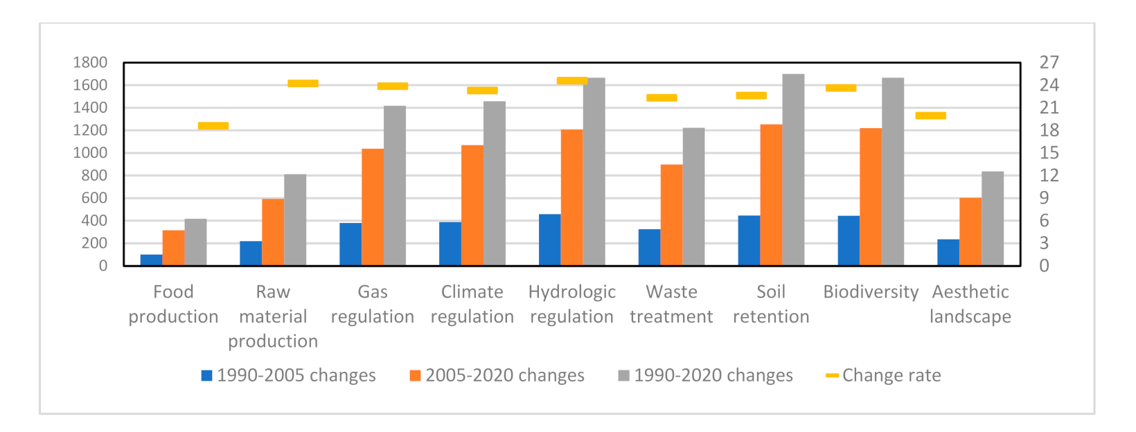
In terms of the rate of change of individual ESVs (Figure 6 and Figure 7), hydrological ESV was one of the most dominant ESV types, exhibiting the largest increase of 24.6%, followed by the raw material production and gas regulation ESVs with increases of 24.22% and 23.86%, respectively, and then the food supply ESV with the smallest change (18.6%). These results indicate that the profit and loss of each type of ESV is affected to varying degrees with the change of land use in “reforestation” and urbanization.
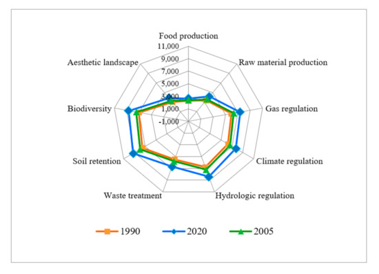
Figure 6.
Comparison of changes in individual ESVs during 1990–2020 (×CNY 106).

Figure 7.
Individual ESV changes during 1990–2020.
In terms of LUCC (Table 6), the total ESV of the Guanzhong Region increased by a total of 11,201.24 × CNY 106 (23.51%) between 1990 and 2020. Forest land had the highest ESV in each year and was the main contributor, followed by agricultural land. Moreover, unused land was associated with the lowest ESV. Over the 30-year period, all LUCC types underwent flow, and the ESV of construction land, watershed and forests increased significantly, while the ESV of unused land decreased. The large differences in ESV among land use types suggest that the substrate has a large influence on ESV.
Table 6.
Changes in ESV for each LUCC during 1990–2020.
3.3. ESV Predictions Based on LUCC
3.3.1. Predicted LUCC Based on CA-Markov
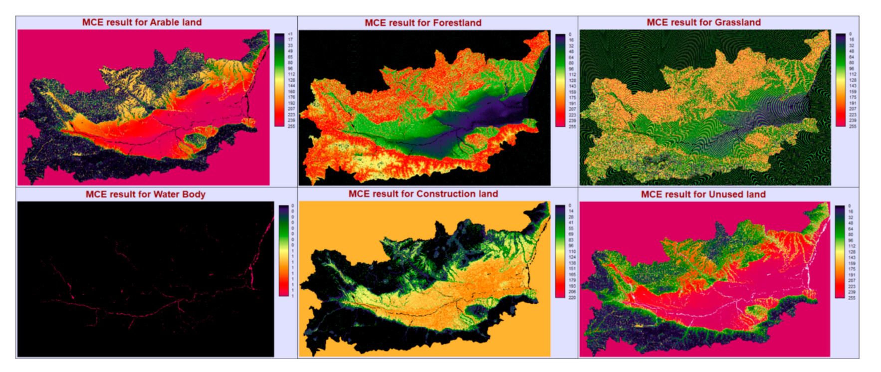
In this study, a continuous filter was used with a standard kernel size of 5 × 5 pixels to determine transition suitability maps by elevation, slope, roads, nature reserves, lighting, and population density using a multi-criteria evaluation (MCE) decision support tool (Figure 8). The kappa index value of 0.905 was calculated and the model passed accuracy validation, indicating that the CA-Markov prediction is valid.
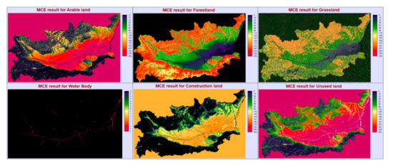
Figure 8.
Suitability maps based on 2015 LUCC using a multi-criteria evaluation (MCE) tool.
Next, the LUCC for 2025 and its comparison with the LUCC of previous study years were scientifically derived (Figure 9, Table 7). The prediction results of the CA-Markov model were relatively clear, where, compared to 2020, the area of forest land increases by 4250.3 hm2, and the construction land increases significantly by 58,332.98 hm2. At the same time, other LUCC decreased to different degrees, of which grassland decreased the most (39,066.51 hm2).
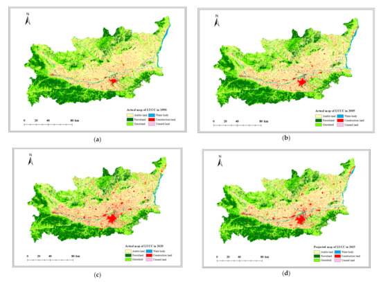
Figure 9.
Comparison of LUCC maps for actual years (1990 (a), 2005 (b), and 2020 (c)) and the projected year (2025 (d)).
Table 7.
Projected LUCC of the Guanzhong Region in 2025 (hm2).
With the rapid economic rise of the Guanzhong region and unprecedented urbanization, the dynamic changes in land use have been remarkable. The relevant data show that large quantities of non-construction land has been converted into construction land, indicating that the LUCC change situation in the region is obviously influenced by human disturbances.
3.3.2. Predicted Spatial Inequalities in ESV
The 2025 LUCC were projected by using the CA-Markov model to further obtain the ESVs in the Guanzhong region (Table 8). The total ESV was predicted to reach 57,040.99 × CNY 106 in 2025, which is a slight decrease of 1811.15 × CNY 106 compared with 2020.
Table 8.
Prediction of ESVs in 2025 for the Guanzhong region (×CNY 106).
Concerning specific land cover categories, forest land provided the highest ESV (28,120.08 × CNY 106), followed by cropland (14,909.59 × CNY 106) and grassland (11,639.98 × CNY 106), while built-up land and unused land only provided 0.75% of the total ESV, which highlights the importance of protecting ecological land to maintain ESV.
In terms of specific ESV types, SR remains the dominant ESV contributor (9087.97 × CNY 106), followed by BP (8495.5 × CNY 106) and HR (7880.22 × CNY 106). All ESVs were predicted to decrease to varying degrees compared to 2020, except for FS, which was predicted to increase by 9.59 × CNY 106, something which is likely related to the growth of cropland FS and the increase in food prices. In addition, among the individual ESVs, HR of watershed, SR of grassland and BP of forest land decreased significantly, which may be related to the transfer of the three types of ecological land to construction land, thus leading to the hardening of roads or the pollution of water bodies, itself resulting in the weakening of the ecological carrying capacity of watersheds, forest land and grassland.
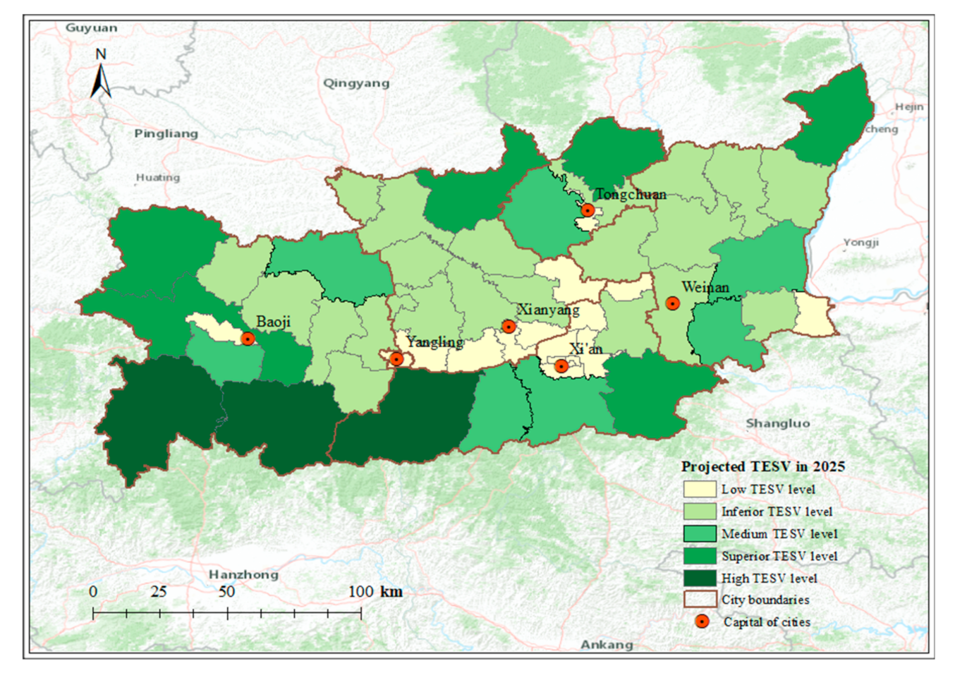
At the level of individual administrative municipality units, the TESV in 2025 shows a clear spatial inequality (Figure 10). Specifically, the administrative capital of the city displays a significantly lower TESV than the surrounding counties. Additionally, inferior levels of TESV are more common in northern areas, for example, some counties in central Xianyang and Weinan degrade from moderate to inferior levels in 2020. Notably, southern Baoji and southwestern Xi’an (three counties) exhibit consistently higher TESV levels, which may be related to the observation that the Tai Bai National Forest Park is located there and is classified as a nature reserve.
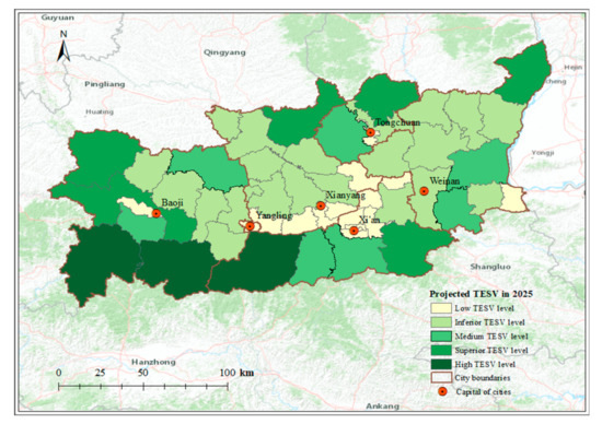
Figure 10.
Projected TESV in 2025.
4. Discussion
4.1. Impact of Demographic Factors on Future ESVs
A critical step in ecosystem assessment is determining the scope of the ESVs’ capabilities and the social demands placed on them by different stakeholders [52,53]. In both cases, it has been shown that ecosystems are influenced by both natural attributes (e.g., climate, LUCC) and social demands [54,55]. Besides climate change, changes in LUCC have become a central contributor to ES [56], which are driven to a large extent by human activities. Therefore, demographic factors pose a major challenge for quantitative prediction of future ESV changes [57].
4.1.1. Population Projection
In order to further investigate the influence of demographic factors on ESV in the Guanzhong region, a future demographic scenario was simulated. According to Equations (11) and (12) and the fitting principle, and using the demographic data of the five cities in the Guanzhong region from 1990 to 2020 as a basis for this study, the following results were obtained: the population of the five cities tends to expand over time and the deficit changes by an equal number, i.e., the ratio always fluctuates between 0.8 and 1.0. Therefore, the application of a logistic function is appropriate for making predictions.
Using Matlab software, it could be seen that the predicted data and actual data curve were in general agreement, and the predicted populations for each city were determined (Table 9). These results suggest that the total resident population in the Guanzhong region will continue to grow. Compared to 2020, the population outflow from the remaining two cities leads to a decrease in population, while Xi’an, Baoji and Weinan exhibit increases, especially Xi’an, which displayed the largest increase of 3.09 million new residents. It is worth noting that Xi’an, as the capital city of the province, has the advantage of its geographical location and various resources, and coupled with its identification as a “national central city” in 2018 [58], the city’s influence has further expanded and its population has swelled significantly. For these reasons, Xi’an is expected to be among China’s mega cities by 2030. These projections coincide with the 14th Five-Year Plan for National Economic and Social Development of Shaanxi Province and Vision 2035 [59].
Table 9.
Cities’ population projection for 2025 (thousands).
However, due to the limited resources provided by ecosystems and their carrying capacity, the problems of decreasing urban green space per capita [22], increasing ecological welfare imbalance [60] and decreasing spatial discount rate of ES functions [61] will become increasingly prominent as the population grows, making it necessary for planners to confront the spatial inequity when considering ES in the context of future population growth [62,63].
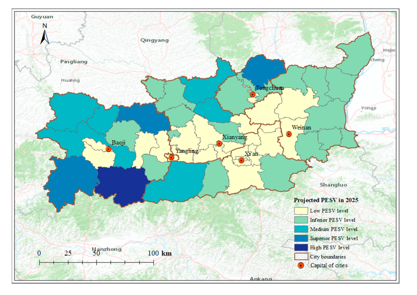
4.1.2. Spatial Inequality of per Capita ESV in 2025
The results of the CA-Markov and logistic model were used to project the per capita ESV in 2025. Here, the results show that the PESV maintained the spatial heterogeneity characteristic of decreasing from west to east and from periphery to inner periphery (Figure 11). By 2025, the highest-level area remains around Baoji City, i.e., Taibai County. Moreover, the low-level counties were projected to grow from 14 in 2020 to 26 in 2025, 10 of which are from Xi’an City. As of 2025, Xi’an city is projected to have the fastest population growth, while Baoji adds only 7% of Xi’an’s population. This implies that urban population pressure has a significant impact on the yield of ES, which is also consistent with previous findings [21,64].
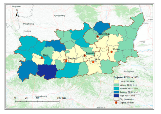
Figure 11.
Projected per capita ESV in 2025.
Xi’an, the administrative, economic and political center of the study area, has a strong urban absorption capacity [65], but remains a spatial depression of ESV [66]. Of the land available for development, Xi’an is the most heavily developed and has displayed the greatest increase in consumption of ESV. This explains why the city of Xi’an can accommodate a larger population but with an upper limit of ESV occupancy per capita. In contrast, the decline in ESV is small in the southern mountainous areas of Baoji and the rural areas in the north, which is likely attributed more to local land use patterns than population [63]. Most of the available land in Xi’an is dedicated to housing, while the developable land in the southern mountainous area of Baoji and the northern rural area is used for forest and farm conservation. In fact, most of the woodlands and grasslands in the southern mountainous areas of Baoji are protected from development by specific environmental policies and designations (e.g., the Zibai Mountain National Nature Reserve, the Huangbai Plateau Original Ecological Landscape Area, and the Taibai Mountain National Forest Park). For these reasons, the overall PESV in Baoji is more favorable and is minimized by urban change as well as population impacts [67].
4.2. Optimization of ESV Based on Demographic Factors and Urban Development
Cities with a large and dense populations usually have less available ecological land [68], and residents of densely populated areas therefore experience limited interactions with nature, which negatively affects their ecological well-being [69,70]. To eliminate this negative effect, ecological land is urgently needed in such cities. Conversely, in cities with constrained development of built-up land, when population pressure increases, there is a need to develop more productive and residential land. The deprivation of high ESV land types such as woodlands and grasslands become stronger in response to the limited availability of low-ESV land types that can be developed [71]. In response to the pressure of these demographic factors, it is necessary for policy makers to have clearer planning directions on the potential of urban ES to alleviate the influence of the demographic expansion on environmental services within the planning area [27].
Here, this study emphasizes the significance of keeping a permanent protection of land with high natural capital, such as the Zibai Mountain National Nature Reserve, the Huangbai Plateau Original Ecological Landscape Area, and the Taibai Mountain National Forest. Even with high levels of population growth, these areas will be able to maintain a greater level of ES provisioning capacity in the future, largely because development in these areas is prohibited. [72]. Therefore, maintaining ES and harmonious relationships while protecting the type of land use proposed in the integrated plan is crucial for the planning strategy [19].
The observation that the decline in ESV was not dramatic throughout the study area underscores the fact that the decline in ESV will be mitigated and masked in general if ecological lands are well maintained and productive and living lands are developed within reasonable limits. As the population will continue to grow in the future, the quality of ESV enhancement should be taken into account as residents experience the impacts of population and land use on ES [73,74]. This consideration may help community planners adapt to changing conditions in order to moderate the effects of population growth on ES in the planning area. For example, urbanization can negatively affect ESV by increasing the demand for construction land, and the rational and intensive use of land resources can be achieved through industrial restructuring, thereby maximizing the market efficiency of ESV, optimizing the industrial structure, and protecting the local ecological environment, which are important components of sustainable land use ecological economy. In addition, domestic provinces have carried out an “environmental protection loan” policy, with a financial risk compensation pool used as a means of credit to provide loans for environmental protection infrastructure construction, ecological protection and restoration and environmental protection industry development. “Environmental protection loans” are conducive to the construction of diversified, market-oriented ecological and environmental protection investment mechanisms to promote the green development of industry. At the same time, the policy is also a useful attempt to “green finance”, focusing on the protection of the ecological environment and environmental pollution control in financial operations, and promoting sustainable social development through the guidance of social and economic resources.
5. Conclusions
The value coefficient methodology put forward by Xie et al. [34] and Costanza et al. [3] provides a viable reference for estimating ESV. Similarly, the CA-Markov prediction model provides a scientific basis for land use planning. Applying the above methods, this study investigated the effects of demographic and land use change factors on ecosystem services. With the sharp increase of urbanization in the Guanzhong region, this paper explores the general pattern of land use change in the region and found that, firstly, the most obvious change among all LUCCs was that of construction land (with an increase of 144,760.51 hm2), and that 1529.64 hm2 of arable land was occupied in the process of transhumance; the comprehensive land use intensity index of ecological land increased from 253.63% in 1990 to 255.86% in 2020, following increasing anthropogenic disturbance. Secondly, this paper found that total ESV increased by RMB 11,201.24×106, with the highest ESV in all periods being associated with forest land. Regulating ecosystem services, accounting for 51.33%, dedicated the most in ESV, while the ESV between counties and districts displayed spatial differences of “low center and high periphery”. Thirdly, this papers results show that: total ESV in 2025 was projected to reach 57,040.99 × CNY 106, with a slight decrease compared with 2020; forest land still provides the highest ESV; ESV of the soil conservation subtype plays a major role; TESV in 2025 is unevenly distributed, with inferior levels spreading northward, while high ESV levels are still maintained in the northern Qinling counties in the south. Fourthly, the results also show that: the high-level per capita ESV area in 2025 remains in Baoji City, with the highest per capita ESV area in Taibai County; the low-level counties were projected to grow from 14 in 2020 to 26 in 2025, with 10 of them being from Xi’an City, which was the main low-value area. Xi’an city can accommodate more population while reaching the upper limit of per capita ESV occupancy, while Baoji has better overall per capita ESV and is least affected by urban change and population growth. Governments should take efforts to maintain the positive impacts of ES and consider the quality of ESV enhancements when residents experience land use changes.
Author Contributions
Conceptualization, Y.C. and Z.L.; methodology, P.L.; software, Y.C.; formal analysis, Y.C.; data curation, J.P. and H.L.; writing—original draft preparation, Y.C.; writing—review and editing, Y.C.; visualization, Y.C.; proofreading, Y.C. and Y.Z.; supervision, Z.L.; project administration, P.L.; funding acquisition, Z.L. All authors have read and agreed to the published version of the manuscript.
Funding
This research was supported by National Natural Science Foundation of China, (Grant No. 51879281, No. 51979221); Ningxia Water Conservancy Science and Technology Project, SBZZ-J-2021-12.
Institutional Review Board Statement
Not applicable.
Informed Consent Statement
Not applicable.
Data Availability Statement
Not applicable.
Acknowledgments
We would like to thank Shannon Elliot at Michigan State University for his assistance with English language and grammatical editing.
Conflicts of Interest
The authors state that they have no known competing financial interests or personal relationships that could affect the work described in this article.
References
- Costanza, R.; d’Arge, R.; de Groot, R.; Farber, S.; Grasso, M.; Hannon, B.; Limburg, K.; Naeem, S.; O’Neill, R.V.; Paruelo, J.; et al. The value of the world’s ecosystem services and natural capital. Nature 1997, 387, 253–260. [Google Scholar] [CrossRef]
- Liu, J.; Li, J.; Qin, K.; Zhou, Z.; Yang, X.; Li, T. Changes in land-uses and ecosystem services under multi-scenarios simulation. Sci. Total Environ. 2017, 586, 522–526. [Google Scholar] [CrossRef] [PubMed]
- Costanza, R.; De Groot, R.; Braat, L.; Kubiszewski, I.; Fioramonti, L.; Sutton, P.; Grasso, M. Twenty years of ecosystem services: How far have we come and how far do we still need to go? Ecosyst. Serv. 2017, 28, 1–16. [Google Scholar] [CrossRef]
- Elmqvist, T.; Setälä, H.; Handel, S.N.; van der Ploeg, S.; Aronson, J.; Blignaut, J.N.; Gómez-Baggethun, E.; Nowak, D.J.; Kronenberg, J.; de Groot, R. Benefits of restoring ecosystem services in urban areas. Curr. Opin. Environ. Sustain. 2015, 14, 101–108. [Google Scholar] [CrossRef] [Green Version]
- Bolund, P.; Hunhammar, S. Ecosystem services in urban areas. Ecol. Econ. 1999, 29, 293–301. [Google Scholar] [CrossRef]
- Bowler, D.E.; Buyung-Ali, L.; Knight, T.M.; Pullin, A.S. Urban greening to cool towns and cities: A systematic review of the empirical evidence. Landsc. Urban Plan. 2010, 97, 147–155. [Google Scholar] [CrossRef]
- Berland, A.; Shiflett, S.A.; Shuster, W.D.; Garmestani, A.S.; Goddard, H.C.; Herrmann, D.L.; Hopton, M.E. The role of trees in urban stormwater management. Landsc. Urban Plan. 2017, 162, 167–177. [Google Scholar] [CrossRef] [Green Version]
- Mcdougall, R.; Kristiansen, P.; Rader, R. Small-scale urban agriculture results in high yields but requires judicious management of inputs to achieve sustainability. Proc. Natl. Acad. Sci. USA 2019, 116, 129–134. [Google Scholar] [CrossRef] [Green Version]
- Wolch, J.R.; Byrne, J.; Newell, J.P. Urban green space, public health, and environmental justice: The challenge of making cities “just green enough”. Landsc. Urban Plan. 2014, 125, 234–244. [Google Scholar] [CrossRef] [Green Version]
- Alam, M.; Dupras, J.; Messier, C. A framework towards a composite indicator for urban ecosystem services. Ecol. Indic. 2016, 60, 38–44. [Google Scholar] [CrossRef]
- Estoque, R.C.; Murayama, Y. Landscape pattern and ecosystem service value changes: Implications for environmental sustainability planning for the rapidly urbanizing summer capital of the Philippines. Landsc. Urban Plan. 2013, 116, 60–72. [Google Scholar] [CrossRef]
- Winkler, R. Valuation of ecosystem goods and services: Part 1: An integrated dynamic approach. Ecol. Econ. 2006, 59, 82–93. [Google Scholar] [CrossRef]
- Cordier, M.; Agúndez, J.A.P.; Hecq, W.; Hamaide, B. A guiding framework for ecosystem services monetization in ecological-economic modeling. Ecosyst. Serv. 2013, 8, 86–96. [Google Scholar] [CrossRef] [Green Version]
- Tallis, H.; Yukuan, W.; Bin, F.; Bo, Z.; Wanze, Z.; Min, C.; Tam, C.; Daily, G. The Natural Capital Project. Bull. Br. Ecol. Soc. 2010, 41, 10–13. [Google Scholar]
- Burkhard, B.; de Groot, R.; Costanza, R.; Seppalt, R.; Jorgensen, S.V.; Potschin, M. Solutions for sustaining natural capital and ecosystem services. Ecol. Indic. 2012, 21, 1–6. [Google Scholar] [CrossRef]
- Seppelt, R.; Fath, B.; Burkhard, B.; Fisher, J.L.; Gret-Regamey, A.; Lautenbach, S.; Pert, P.; Hotes, S.; Spangenberg, J.; Verburg, P.H.; et al. Form follows function? Proposing a blueprint for ecosystem service assessment based on reviews and case studies. Ecol. Indic. 2012, 21, 145–154. [Google Scholar] [CrossRef]
- Ranganathan, J.; Raudsepp-Hearne, C.; Lucas, N.; Irwin, F.; Zurek, M.; Bennett, K.; Ash, N.; West, P. Ecosystem Services: A Guide for Decision Makers; World Resources Institute: Washington, DC, USA, 2008; 96p. [Google Scholar]
- Nik, V.; Catherine, R.P.; Caren, C.H. On Enabling comparative gene expression studies of thyroid hormone action through the development of a flexible real-time quantitative PCR assay for use across multiple anuran indicator and sentinel species. Aquat. Toxicol. 2014, 148, 162–173. [Google Scholar] [CrossRef]
- de Groot, R.S.; Alkemade, R.; Braat, L.; Hein, L.; Willemen, L. Challenges in integrating the concept of ecosystem services and values in landscape planning, management and decision making. Ecol. Complex. 2010, 7, 260–272. [Google Scholar] [CrossRef]
- Goldstein, J.H.; Caldarone, G.; Duarte, T.K.; Ennaanay, D.; Mendoza, G.; Polasky, S.; Wolny, S.; Daily, G.C. Integrating ecosystem-service tradeoffs into land-use decisions. Proc. Natl. Acad. Sci. USA 2012, 9, 7565–7757. [Google Scholar] [CrossRef] [Green Version]
- Wang, J.; Zhou, W.; Pickett, S.T.; Yu, W.; Li, W. A multiscale analysis of urbanization effects on ecosystem services supply in an urban megaregion. Sci. Total Environ. 2019, 662, 824–833. [Google Scholar] [CrossRef]
- Chen, Y.; Ge, Y.; Yang, G.; Wu, Z.; Du, Y.; Mao, F.; Liu, S.; Xu, R.; Qu, Z.; Xu, B.; et al. Inequalities of urban green space area and ecosystem services along urban center-edge gradients. Landsc. Urban Plan. 2022, 217, 104266. [Google Scholar] [CrossRef]
- Ontario Ministry for Environment and Energy. Toward an Ecosystem Approach to Land-use Planning; Environmental Planning and Analysis Branch, Ontario Ministry of Environment and Energy: Toronto, ON, USA, 1994. [Google Scholar]
- TEEB. The Economics of Ecosystems and Biodiversity Ecological and Economic Foundations; Pushpam, K., Ed.; Earthscan: London, UK; Washington, DC, USA,, 2010. [Google Scholar]
- Tian, L.; Chen, J.; Yu, S.X. Coupled dynamics of urban landscape pattern and socioeconomic drivers in Shenzhen, China. Landsc. Ecol. 2014, 29, 715–727. [Google Scholar] [CrossRef]
- Gourevitch, J.D.; Alonso-Rodríguez, A.M.; Aristizábal, N.; de Wit, L.A.; Kinnebrew, E.; Littlefield, C.E.; Moore, M.; Nicholson, C.C.; Schwartz, A.J.; Ricketts, T.H. Projected losses of ecosystem services in the US disproportionately affect non-white and lower-income populations. Nat. Commun. 2021, 12, 3511. [Google Scholar] [CrossRef] [PubMed]
- Jantz, C.A.; Manuel, J.J. Estimating impacts of population growth and land use policy on ecosystem services: A community-level case study in Virginia, USA. Ecosyst. Serv. 2013, 5, 110–123. [Google Scholar] [CrossRef]
- Mcdonnell, M.J.; Macgregor-Fors, I. The ecological future of cities. Science 2016, 352, 936–938. [Google Scholar] [CrossRef]
- Wu, J. Urban ecology and sustainability: The state-of-the-science and future directions. Landsc. Urban Plan. 2014, 125, 209–221. [Google Scholar] [CrossRef]
- Narducci, J.; Quintas-Soriano, C.; Castro, A.; Som-Castellano, R.; Brandt, J. Implications of urban growth and farmland loss for ecosystem services in the western United States. Land Use Policy 2019, 86, 1–11. [Google Scholar] [CrossRef]
- Xiao, F.M.; Jian, T.Z.; Hong, B.Z.; Wei, Y.; Cheng, Y.Z. Trade-offs and synergies in ecosystem service values of inland lake wetlands in Central Asia under land use/cover change: A case study on Ebinur Lake, China. Glob. Ecol. Conserv. 2020, 24, e01253. [Google Scholar] [CrossRef]
- Li, Y.L.; Yang, F.L.; Yang, L.N.; Shang, X.Q.; Hu, G.; Jia, L.J. Spatial pattern changes of land use in Yulin City in the last 40a and analysis of influencing factors. Geogr. Arid. Reg. 2021, 44, 1011–1021. (In Chinese) [Google Scholar]
- Wang, Y.; Dai, E.; Yin, L.; Ma, L. Land use/land cover change and the effects on ecosystem services in the Hengduan Mountain region, China. Ecosyst. Serv. 2018, 34, 55–67. [Google Scholar] [CrossRef]
- Li, W.; Chen, T.; Ma, X. Spatial pattern evolution and driving mechanism of land use in urban tourism complexes: The case of Xi’an Qujiang. Geogr. Res. 2019, 38, 1103–1118. (In Chinese) [Google Scholar]
- Fan, Y.; Liu, J. Land use in Tibet Autonomous Region; Science Press: Beijing, China, 1994. [Google Scholar]
- Xie, G.D.; Lu, C.X.; Leng, Y.F.; Zheng, D.; Li, S.C. Ecological assets valuation of the Tibetan Plateau. J. Nat. Resour. 2003, 18, 189–196. [Google Scholar] [CrossRef]
- Xie, G.D.; Zhang, C.X.; Zhen, L.; Zhang, L.M. Dynamic changes in the value of China’s ecosystem services—ScienceDirect. Ecosyst. Serv. 2017, 26, 146–154. [Google Scholar] [CrossRef]
- Xu, X.G.; Cui, C.W.; Xu, L.F.; Ma, L.Y. Method study on relative assessment for ecosystem service: A case of green space in Beijing, China. Environ. Earth Sci. 2013, 68, 1913–1924. [Google Scholar] [CrossRef]
- Wolfram, S. Statistical mechanics of cellular automata. Rev. Mod. Phys. 1983, 55, 601. [Google Scholar] [CrossRef]
- Li, X.; Yeh, A.G.-O. Neural-network-based cellular automata for simulating multiple land use changes using GIS. Int. J. Geogr. Inf. Sci. 2002, 16, 323–343. [Google Scholar] [CrossRef]
- Yang, X.; Zheng, X.Q.; Chen, R. A land use change model: Integrating landscape pattern indexes and Markov-CA. Ecol. Model. 2014, 283, 1–7. [Google Scholar] [CrossRef]
- Wijesekara, G.N.; Gupta, A.; Valeo, C.; Hasbani, J.G.; Qiao, Y.; Delaney, P.; Marceau, D.J. Assessing the impact of future land-use changes on hydrological processes in the Elbow River watershed in southern Alberta, Canada. J. Hydrol. 2012, 412–413, 220–232. [Google Scholar] [CrossRef]
- Sannigrahi, S.; Zhang, Q.; Joshi, P.K.; Sutton, P.; Keesstra, S.; Roy, P.; Pilla, F.; Basu, B.; Wang, Y.; Jha, S.; et al. Examining effects of climate change and land use dynamic on biophysical and economic values of ecosystem services of a natural reserve region. J. Clean. Prod. 2020, 257, 120424. [Google Scholar] [CrossRef]
- Saa, B.; Nb, C. Towards Scalable Deployment of Hidden Markov Models in Occupancy Estimation: A Novel Methodology Applied to the Study Case of Occupancy Detection. Energy Build. 2021, 254, 111594. [Google Scholar] [CrossRef]
- Nor, A.N.M.; Corstanje, R.; Harris, J.A.; Brewer, T. Impact of rapid urban expansion on green space structure. Ecol. Indic. 2017, 81, 274–284. [Google Scholar] [CrossRef]
- Mas, J.F.; Kolb, M.; Paegelow, M.; Camacho Olmedo, M.T.; Houet, T. Inductive pattern-based land use / cover change models: A comparison of four software packages. Environ. Model. Softw. 2014, 51, 94–111. [Google Scholar] [CrossRef] [Green Version]
- Lcmm, A.; Tcd, B. On the Global Time Evolution of the Covid-19 Pandemic: Logistic Modeling. Technol. Forecast. Soc. Chang. 2022, 175, 121387. [Google Scholar] [CrossRef]
- Salas-Eljatib, C.; Fuentes-Ramirez, A.; Gregoire, T.G.; Altamirano, A. A study on the effects of unbalanced data when fitting logistic regression models in ecology. Ecol. Indic. 2018, 85, 502–508. [Google Scholar] [CrossRef]
- Marcos, R.; Jiménez-Ruanobc, A.; Peña-Angulob, D.; la Riva, J. A comprehensive spatial-temporal analysis of driving factors of human-caused wildfires in Spain using Geographically Weighted Logistic Regression. J. Environ. Manag. 2018, 225, 177–192. [Google Scholar] [CrossRef] [Green Version]
- Soga, M.; Gaston, K.J. Extinction of experience: The loss of human-nature interactions. Front. Ecol. Environ. 2016, 14, 94–101. [Google Scholar] [CrossRef] [Green Version]
- Thorn, A.M.; Wake, C.P.; Grimm, C.D.; Mitchell, C.R.; Mineau, M.M.; Ollinger, S.V. Development of scenarios for land cover, population density, impervious cover, and conservation in New Hampshire, 2010–2100. Ecol. Soc. 2017, 22, 19. [Google Scholar] [CrossRef]
- Castro, A.J.; Verburg, P.; Martín-López, B.; García-Llorente, M.; Cabello, J.; Vaughn, C.; López, E. Ecosystem service trade-offs from the supply to social demand: A landscape-scale spatial analysis. Landsc. Urban Plan. 2014, 132, 102–110. [Google Scholar] [CrossRef]
- Martín-López, B.; Gómez-Baggethun, E.; García-Llorente, M.; Montes, C. Trade-offs across value-domains in ecosystem services assessment. Ecol. Indic. 2014, 37, 220–228. [Google Scholar] [CrossRef]
- Burkhard, B.; Kroll, F.; Nedkov, S.; Müller, F. Mapping ecosystem service supply, demand and budgets. Ecol. Indic. 2012, 21, 17–29. [Google Scholar] [CrossRef]
- Castro, A.J.; García-Llorente, M.; Martín-López, B.; Palomo, I.; Iniesta-Arandía, I. Multidimensional approaches in ecosystem services assessment. In Earth Observation of Ecosystem Services; di Bella, C., Alcaraz-Segura, D., Eds.; CRC Press and Taylor and Francis Group: Boca Raton, FL, USA, 2013; pp. 441–468. [Google Scholar]
- Vitousek, P.M.; Mooney, H.A.; Lubchenco, J.; Melillo, J.M. Human domination of Earth’s ecosystems. Science 1997, 277, 494–499. [Google Scholar] [CrossRef] [Green Version]
- Polasky, S.; Carpenter, S.R.; Folke, C.; Keeler, B. Decision-making under great uncertainty: Environmental management in an era of global change. Trends Ecol. Evol. 2011, 26, 398–404. [Google Scholar] [CrossRef] [PubMed]
- Available online: http://xaic.xa.gov.cn/zxdt/tzzx/5db00e07f99d6527b6cc4ea2.html (accessed on 15 January 2022).
- Available online: http://www.shaanxi.gov.cn/zfxxgk/fdzdgknr/zcwj/szfwj/szf/202103/t20210316_2156630.html (accessed on 23 January 2022).
- Bian, J.; Zhang, Y.; Shuai, C.; Shen, L.; Ren, H.; Wang, Y. Have cities effectively improved ecological well-being performance? Empirical analysis of 278 Chinese cities. J. Clean. Prod. 2019, 245, 118913. [Google Scholar] [CrossRef]
- Yamaguchi, R.; Shah, P. Spatial discounting of ecosystem services. Resour. Energy Econ. 2020, 62, 101186. [Google Scholar] [CrossRef]
- Sun, Y.; Li, J.; Liu, X.; Ren, Z.; Zhou, Z.; Duan, Y. Spatially Explicit Analysis of Trade-Offs and Synergies among Multiple Ecosystem Services in Shaanxi Valley Basins. Forests 2020, 11, 209. [Google Scholar] [CrossRef] [Green Version]
- Chen, Y.; Li, Z.; Li, P.; Zhang, Z.; Zhang, Y. Identification of Coupling and Influencing Factors between Urbanization and Ecosystem Services in Guanzhong, China. Sustainability 2021, 13, 10637. [Google Scholar] [CrossRef]
- Richards, D.; Masoudi, M.; Oh, R.R.Y.; Yando, E.S.; Zhang, J.; Friess, D.A.; Grêt-Regamey, A.; Tan, P.Y.; Edwards, P.J. Global Variation in Climate, Human Development, and Population Density Has Implications for Urban Ecosystem Services. Sustainability 2019, 11, 6200. [Google Scholar] [CrossRef] [Green Version]
- Kapsalyamova, Z.; Mezher, T.; Al Hosany, N.; Tsai, I.-T. Are low carbon cities attractive to cleantech firms? Empirical evidence from a survey. Sustain. Cities Soc. 2014, 13, 125–138. [Google Scholar] [CrossRef]
- Dadao, L.U.; Chen, M. Several viewpoints on the background of compiling the “National New Urbanization Planning (2014–2020)”. Acta Geogr. Sin. 2015, 70, 179–185. [Google Scholar] [CrossRef]
- Tian, Y.; Zhou, D.; Jiang, G. Conflict or Coordination? Multiscale assessment of the spatio-temporal coupling relationship between urbanization and ecosystem services: The case of the Jingjinji Region, China. Ecol. Indic. 2020, 117, 106543. [Google Scholar] [CrossRef]
- Richards, D.R.; Passy, P.; Oh, R. Impacts of population density and wealth on the quantity and structure of urban green space in tropical Southeast Asia. Landsc. Urban Plan. 2017, 157, 553–560. [Google Scholar] [CrossRef]
- Maas, J.; van Dillen, S.M.E.; Verheij, R.A.; Groenewegen, P.P. Social contacts as a possible mechanism behind the relation between green space and health. Health Place 2009, 15, 586–595. [Google Scholar] [CrossRef] [PubMed] [Green Version]
- Alcock, I.; White, M.P.; Wheeler, B.W.; Fleming, L.E.; Depledge, M.H. Longitudinal Effects on Mental Health of Moving to Greener and Less Green Urban Areas. Environ. Sci. Technol. 2014, 48, 1247–1255. [Google Scholar] [CrossRef] [PubMed] [Green Version]
- Jim, C.Y. Green-space preservation and allocation for sustainable greening of compact cities. Cities 2004, 21, 311–320. [Google Scholar] [CrossRef]
- Chuai, X.; Huang, X.; Wu, C.; Li, J.; Lu, Q.; Qi, X.; Zhang, M.; Zuo, T.; Lu, J. Land use and ecosystems services value changes and ecological land management in coastal Jiangsu, China. Habitat Int. 2016, 57, 164–174. [Google Scholar] [CrossRef]
- Bai, Y.; Deng, X.; Jiang, S.; Zhang, Q.; Wang, Z. Exploring the relationship between urbanization and urban eco-efficiency: Evidence from prefecture-level cities in China. J. Clean. Prod. 2018, 195, 487–1496. [Google Scholar] [CrossRef]
- Cao, Y.; Kong, L.; Zhang, L.; Ouyang, Z. The balance between economic development and ecosystem service value in the process of land urbanization: A case study of China’s land urbanization from 2000 to 2015. Land Use Policy 2021, 108, 105536. [Google Scholar] [CrossRef]


Publisher’s Note: MDPI stays neutral with regard to jurisdictional claims in published maps and institutional affiliations. |
© 2022 by the authors. Licensee MDPI, Basel, Switzerland. This article is an open access article distributed under the terms and conditions of the Creative Commons Attribution (CC BY) license (https://creativecommons.org/licenses/by/4.0/).