Relationship between Water Use and per Capita Income with Environmental Kuznets Curve of Developing Countries: A Case Study in Jiangsu Province, China

Abstract

The relationship between economic growth and environmental variation is an important issue of sustainable development for human beings, especially in developing countries. However, developing countries usually use the standards of developed countries when dealing with environmental issues, which makes the relationship exhibit different characteristics than it does in developed countries. In order to realize a balance relationship between water use and income per capita in developing countries, a multivariable environmental Kuznets curve (EKC) simulation model based on the grey absolute correlation method was modified to improve the description of the balance relationship between water use and per capita income in the Jiangsu Province of China from 2005 to 2017. The results showed that the industrial and agricultural water uses first increased and then decreased, which agreed with an inverted “U” characteristic. The industrial water use was in the declining stage of the inverted “U” characteristic, while the agricultural water use was in a transition phase of the inverted “U” characteristic. However, the domestic water use showed an increasing trend, and it is difficult to estimate whether it showed an inverted “U” characteristic. Simultaneously, different watershed partitions in Jiangsu Province presented different EKC characteristics. In the three different watershed zoning regions of Jiangsu Province, the total water use of the Tai Lake Basin and the Yangtze River Basin exhibited the typical inverted “U” characteristic, while the Huai River Basin was just in the increasing stage. Moreover, the improved multivariable EKC model was suitable to describe the inverted U-shaped variation characteristics of water use, and the developed model outperformed the univariate EKC model in the study area. Based on the characteristics of the EKC, policy ideas for enhancing the coordination among water resources, the economy, and the ecological environment were proposed in order to achieve sustainable development.

1. Introduction

Water security is the most fundamentally guaranteed factor for the development of countries all over the world. In recent years, while pursuing rapid economic development, countries around the world have overexploited water resources, which leads to a series environmental problems like decreasing groundwater tables and water pollution [1,2]. Water becomes a kind of scarce resource in the context of growth in population and great development demand [3,4]. The relationship between water and growth is gaining increasing focus due to the rising water pressure, and the environmental Kuznets curve (EKC) is a significant instrument in understanding this relationship [5,6,7,8].

According to the EKC theory, the environment degrades rapidly with economic growth at the initial stage; when economic growth reaches a certain level, the environmental deterioration caused in the initial stage of development will be relieved and tend to be improved [9,10,11,12]. The EKC theory is widely analyzed in environment pollution fields like air pollution [13,14,15] and water pollution [2,16,17], and EKC studies on water resources increase as the severity of water scarcity grows. The EKC theory implies that water resource problems caused in the initial stage could be alleviated or solved by further development, which could provide guidance for water policy design [18]. Therefore, numerous theoretical and empirical studies have tried to examine the possibility of the existence of an EKC between water use and growth, while their results generally differentiate between regions due to regional differences, which causes the EKC theory to remain controversial [19,20,21,22,23]. However, the existence of the EKC and the location of the EKC curve tipping point are meaningful for developing countries due to their serious water pressure and great development demand, necessitating further research on the EKC relationship between water use and growth in developing countries.

On the basis of the existence of the EKC, the shape and characteristics of the EKC are a critical foundation for the designation of future water policy. The EKC having a different shape and characteristics implies a different evolutionary orientation of water pressure, which generally requires different response strategy [18,19,20,22,23]. However, most of existing research mainly focus on the EKC’s existence at the national or regional level [3,4,18,20,23,24], and only a small number of studies analyze the characteristics of the EKC curve within a region. In these limited studies, the EKC relationship between the water consumption of a specific sector (e.g., municipal and industrial water consumption) and growth is the main focus [20,21], and there is insufficient research on the multisectoral water-growth EKC curves within a region. In addition, current studies often ignore the spatial characteristics of water, and the EKC relationship between water use and growth in different watershed zoning regions remains unclear. Consequently, it is necessary to further explore the regional characteristics of water-growth EKC curves in developing countries from the sectoral, watershed zoning, and other perspectives.

The simulation model is critical in EKC theory testing and characteristic analysis. However, many previous studies have utilized simplified univariate curve models to simulate the relationship between water use and economic growth, i.e., using a single index to represent water use and taking the level of economic development as the only factor affecting the change of water use [4,19,23,25,26,27,28,29]. According to this point, the simplified univariate EKC model assumes that the economic development pattern and its impact on water use in different regions are basically the same. This hypothesis ignores the actual complex relationship between water resources and the economic and social systems, which makes the results of the univariate EKC model unable to conform to the distribution characteristics of a traditional EKC. This kind of model is more suitable for verifying the existence of the EKC, but it is difficult to accurately describe the long-term stable change trend in the inverted “U”-shaped curve in the descending phase. Therefore, the research on EKC has turned to exploring multivariate simulation models to describe the relationship between water use and economic development more accurately, including simplified univariate quadratic curve models and cubic curve models [30,31,32,33].

On the basis of the demand from developing countries and the above research gaps, taking Jiangsu Province, China, as the case study area, this study established an improved multivariate EKC simulation model to examine the EKC relationship between water use and economic growth and investigated EKC curve characteristics from the perspectives of sectors and watershed zonings. Specifically, based on the data of water use and social economy, science and technology, and the natural endowment of water resources from 2005 to 2017 in Jiangsu Province, the driving factors of water use in different industries were recognized quantitatively. Then, simulation variables were selected from the driving factors as the input to the multivariable EKC model. The improved model built in this study could provide better understanding of the EKC characteristics in developing countries, and the results provide a reference for Jiangsu Province to favorably pass the turning point of the EKC curve in advance and enter the next stage.

2. EKC Model and Improvements

Quadratic and cubic curve models are often used to simulate and analyze EKC characteristics because of their simple structure, simple simulation, and strong intuitive graphics.

2.1. Quadratic EKC Model

The quadratic curve EKC model is suitable for environmental indicators with obvious inverted U-shaped characteristics. The quadratic Leve-type model of the environmental Kuznets curve is given by [34]:

$$E={\beta }_0+{\beta }_1{X}_t+{\beta }_2{X}_t^2+\epsilon$$

(1)

where E is the explained variable, such as the environmental quality index or water use index; X_t is the explanatory variable, such as the economic development level; β₀ is a constant term; β₁ and β₂ are coefficients; and ε is the error term and follows the normal distribution.

If β₁ > 0 and β₂ < 0, environmental indicators and economic indicators show an inverted U-shaped relationship, which is consistent with traditional EKC characteristics. This means that the environmental quality degrades first and then improves with the development of the economy, and its turning point is Xt* = −β₁/(2β₂). If β₁ < 0 and β₂ > 0, there is a positive U-shaped relationship between the environmental and economic indicators, which is inconsistent with traditional EKC characteristics. This means that the environmental quality first improves with the development of the economy and then continues to degrade.

Given that logarithmic data have the advantages of reduction of heteroscedasticity, asymmetric distribution, and data volatility [35], some scholars used the natural logarithm of E and X_t in Equation (1). The quadratic log model is rewritten as follows:

$$lnE={\beta }_0+{\beta }_{1}ln{X}_t+{\beta }_2{\left(ln{X}_t\right)}^2+\epsilon$$

(2)

when Equation (2) is used to describe the inverted “U” curve, the turning point is X_t* = exp(−β₁/β₂).

2.2. Cubic EKC Model

It has been proven that not all EKC characteristics of environmental indicators are inverted U-shaped. In order to study non-inverted U-shaped environmental indicators, Grossman and Kruger [36] introduced the cubic curve model to study the dynamic changes of the relationship between economic development and environmental quality. The cubic model is also divided into two types: the Leve type and the Log type. The EKC cubic Leve model is generally expressed as

$$E={\beta }_0+{\beta }_1{X}_t+{\beta }_2{X}_t^2+{\beta }_3{X}_t^3+\epsilon$$

(3)

If β₁ > 0, β₂ < 0, and β₃ > 0, there is a positive N-type relationship between environmental and economic indicators. That means environmental quality first degrades and then improves with the development of the economy, and then it degrades again. Furthermore, the two turning points are:

$$X_t=\frac{-2{\beta }_2\pm \sqrt{4{\beta }_2^2-12{\beta }_1{\beta }_2}}{6{\beta }_3}$$

(4)

If β₁ < 0, β₂ > 0, and β₃ < 0, the relationship curve between the two turning points is inverted N-type, and the environmental quality improves first, then degrades, and then improves again with economic development.

Taking the natural logarithm of the variables in Equation (3), the Log formula of the cubic curve model is obtained:

$$lnE={\beta }_0+{\beta }_{1}ln{X}_t+{\beta }_2{\left(ln{X}_t\right)}^2+{\beta }_3{\left(ln{X}_t\right)}^3+\epsilon$$

(5)

According to the expressions of the quadratic curve model and cubic curve model, the quadratic curve model is a special form of the cubic curve model. When β₃ = 0 in the cubic curve model and neither β₁ nor β₂ is zero, the cubic curve model is transformed into the quadratic curve model. The quadratic curve model is more suitable to describe the complete inverted U-shaped characteristics of water use change (first increase when the process of economic development enters the industrial economy era and then decrease when entering the information era).

2.3. Improved EKC Model

In this study, the univariate model was enhanced to a multivariate model, which made up for the deficiency of the univariate EKC model. First, the independent variable, per capita income, of the original model was retained as the indicator of economic development stages. Afterwards, the driving factors of water use in the study area were quantitatively analyzed. The main and secondary factors that affected the water use in the study area were selected as variable indicators. Finally, the three-variable quadratic logarithmic curve model and cubic logarithmic curve model were constructed. In this way, the original univariate model was transformed into a three-variable model. The improved EKC quadratic logarithmic curve model and the cubic logarithmic curve models are expressed as Equations (6) and (7), respectively:

$$lnE={\beta }_0+{\beta }_{1}lnX+{\beta }_2{\left(lnX\right)}^2+{\beta }_{3}lnY+{\beta }_{4}lnZ+ℰ$$

(6)

$$lnE={\beta }_0+{\beta }_{1}lnX+{\beta }_2{\left(lnX\right)}^2+{\beta }_3{\left(lnX\right)}^3+{\beta }_{4}lnY+{\beta }_{5}lnZ+ℰ$$

(7)

where E is the explained variable, water use index; X is explanatory variable 1, per capita GDP, representing the level of economic development; Y and Z are explanatory variables 2 and 3, respectively, representing the main and secondary factors influencing regional water use except per capita GDP; β₀ is a constant term; β₁, β₂, β₃, β₄, and β₅ are the coefficients; and ε is an error term that follows the normal distribution and is generally zero in calculation. According to the differences of different socio-economic development stages in the study area, a corresponding quadratic or cubic logarithmic curve model was selected.

In the conditions of different economic development levels in different regions, the main and secondary factors affecting regional water use are different. This means that explanatory variables Y and Z change dynamically when the improved EKC model is used. Therefore, when Equations (6) and (7) are used to study the dynamic changes in the relationship between economic development and environmental quality, it is necessary to quantitatively analyze the main and secondary factors that affect the changes in water use.

In this study, the grey relational analysis method was used to quantitatively evaluate the factors of water use changes under rapid economic and social development. Weight analysis was also conducted to solve the multivariate problems. This method has the advantages of dealing with uncertainties, no collinearity, unrestricted factors, and simple calculation. The calculation steps of the driving factors of water use in different industries are as follows:

Step 1: Determine the reference sequence of water use factors (X₀) and the comparison sequence (X_i).

$$X_0=\left\{X_0\left(k\right),k=1,2,\dots ,n\right\}$$

(8)

$$X_i=\left\{X_i\left(k\right),k=1,2,\dots ,n\right\}i=1,2,\dots ,m$$

(9)

where n is the period length of the sequence, and i is the number of comparison sequences.

Step 2: Dimensionless treatment. This step is used to eliminate the influence of dimensions and magnitudes on the analysis results of reference and comparison sequences, as well as to increase the comparability between two sequences.

$$y_0=\left\{X_0\left(k\right)/X_0\left(1\right),k=1,2,\dots ,n\right\}$$

(10)

$$y_i=\left\{X_i\left(k\right)/X_i\left(1\right),k=1,2,\dots ,n\right\}i=1,2,\dots ,m$$

(11)

Step 3: Calculate the trend of reference and comparison sequences in each time period.

$$\alpha \left(y_0\left(k+1\right)\right)=y_0\left(k+1\right)-y_0\left(k\right)1,2,\dots ,n-1.$$

(12)

$$\alpha \left(y_i\left(k+1\right)\right)=y_i\left(k+1\right)-y_i\left(k\right)i1,2,\dots ,m$$

(13)

Step 4: Calculate the correlation coefficient for each time period.

$${\xi }_{\left(X_0,X_i\right)}=\frac{1}{1+\left|\alpha \left(y_0\left(k+1\right)\right)-\alpha \left(y_i\left(k+1\right)\right)\right|}k=1,2,\dots ,n-1;i=1,2,\dots ,m$$

(14)

where ${\xi }_{\left(X_0,X_i\right)}$ is the correlation coefficient between the reference sequence X₀ and the comparison sequence X_i.

Step 5: Calculate the degree of relevance. The value of the correlation coefficient indicates the degree of similarity between the reference and comparison sequences. A greater correlation value means that the indicator corresponding to the comparison sequence has a more significant impact on the reference sequence indicator. The relevance degree is calculated as

$${\gamma }_{(X_0,X_i)}=\frac{1}{n-1}{\sum }_{k=1}^{n-1}{\xi }_{(X_0,X_i)}(k+1)i=1,2,\dots ,m$$

(15)

where ${\gamma }_{\left(X_0,X_i\right)}$ is the degree of relevance between the reference sequence X₀ and comparison sequence X_i.

Step 6: Improve the relevance degree with a weighted approach.

The grey absolute correlation calculated with Equation (15) is the average correlation coefficient for each time period of the reference and comparison sequences. It is susceptible to comparison sequence correlation coefficients at maximum or minimum values. In order to reduce the influence of the aforementioned factors on the calculated correlation degree, this study introduced a slope similarity degree between the reference and comparison sequences in different time periods. Thus, the time period correlation coefficient is weighted and improved to enhance the accuracy of the relevance evaluation results. The weight determination method is expressed as

$${\omega }_i\left(k+1\right)=\frac{w_i\left(k+1\right)}{{{\displaystyle \sum }}_{k=1}^{n-1}{w}_i\left(k+1\right)}k=1,2,\dots ,n-1;i=1,2,\dots ,m$$

(16)

where ω_i (k + 1) is the weight of the timeframe correlation coefficient ${\xi }_{\left(X_0,X_i\right)}$ (k + 1). $w_i\left(k+1\right)$ is the slope similarity degree between the reference and contrast sequence in different time periods and can be calculated as

$$w_i\left(k+1\right)=\frac{1}{1+\left|1-\frac{\alpha \left(y_0\left(k+1\right)\right)}{\alpha \left(y_i\left(k+1\right)\right)}\right|},i=1,2,\dots ,m$$

(17)

The correlation degree after weighting is calculated as

$${\gamma }_{\left(X_0,X_i\right)}={{\displaystyle \sum }}_{k=1}^{n-1}{\omega }_i\left(k+1\right){\xi }_{\left(X_0,X_i\right)}\left(k+1\right),k=1,2,\dots ,n-1;i=1,2,\dots ,m$$

(18)

where ${\gamma }_{\left(X_0,X_i\right)}$ is the relevance degree between the reference sequence X₀ and comparison sequence X_i, ${\xi }_{\left(X_0,X_i\right)}$ (k + 1) is the correlation coefficient between the reference sequence X₀ and comparison sequence X_i in different time periods, and ω_i(k + 1) is the weight value of the comparison sequence X_i in different periods.

The data on socio-economic development and water resource development and utilization in Jiangsu Province were collected from the Jiangsu Statistical Yearbook and Jiangsu Water Resources Bulletin. First, Equation (18) was used to quantitatively analyze the factors affecting water use from 2005 to 2017. The main and secondary factors were selected as the explanatory variables Y and Z of the EKC model. Afterwards, Equations (6) and (7) were used to simulate the EKC of water use in Jiangsu Province. Given that the expected function was not a straight line from Equations (6) and (7), the parameter value of the least squares estimation could not be directly calculated. Therefore, the LIMDEP (LIMited DEPendent variable modeling) statistical software was used to perform nonlinear regression simulations. The goodness of fit test of the regression model was carried out with the determination coefficient (R²) and the Akchi information criterion (AIC), and the significance test was carried out with F-statistic.

2.4. Selection of Explanatory Variables for EKC Model

Jiangsu Province is located in the Yangtze River Delta region of China, covering an area of 107,200 km². By the end of 2020, the province had 84.8 million permanent residents and a per capita GDP of CNY 116,400. It is one of the regions with the most dynamic economic development, the highest degree of openness, and the strongest innovation capacity in China. Different water resource endowments and social and economic development conditions in different regions lead to different regional water resource utilization. Therefore, Jiangsu Province was divided into three different sub-regions for analyzing EKC characteristics, and provincial analysis was also conducted. According to the water system and administrative divisions in Jiangsu Province, the three sub-regions are the Tai Lake Basin, the Yangtze River Basin, and the Huai River Basin (Figure 1).

Given that many factors affected water use changes in Jiangsu Province, water use was divided into four categories: regional total water use, industrial water use, agricultural water use, and domestic water use. The factors influencing the changes in different types of water use were categorized into three aspects: social economy, science and technology, and natural endowment of water resources. Representative indicators affecting different types of water use were selected with comprehensive consideration of regional socio-economic development levels, industrial structures, agricultural planting structures, application and promotion of science and technology, local water resources, and available statistical data. The reference sequence was adopted as the water use index, and the comparison sequence was selected as the representative index influencing the water use change. The influence degrees of different indices on each type of water use were quantitatively calculated with the improved grey correlation analysis method. The indices with the first and second influence degrees were selected as the explanatory variables Y and Z, corresponding to the four types of water use.

Table 1. Value of weighted grey absolute correlation degree between different water uses and their driving factors.

Indices		Total Water Use (ET)	Agricultural Water Use (EA)	Industrial Water Use (EI)	Domestic Water Use (EH)
Social and Economy Index	Per Capita GDP	0.8187	0.8086	0.7941	0.8107
	Agriculture Added Value(AAV)	-	0.9543	-	-
	AAV proportion in GDP	0.9440	0.9479	-	-
	Industrial Added Value(IAV)	-	-	0.7528	-
	IAV proportion in GDP	0.9584	-	0.9891	-
	Service industry Added Value proportion in GDP	0.9718	-	-	-
	Permanent population	-	-	-	0.9724
	Urbanization rate	0.9639	-	-	0.9811
	Irrigated Area	0.9876	0.9826	-	-
Science and Technology Index	Water use per unit of IAV	0.9326	-	0.9536	-
	Water quota for urban residents	0.9666	-	-	0.9453
	Water use per unit of irrigation area	0.9597	0.9907	-	-
Water Resources Endowment Index	Per Capita Water Resources	0.7105	0.7200	0.7185	0.7183
	Precipitation	-	0.8781	-	-

Note: GDP has been converted to comparable prices in 2000, and bold italic numbers are the main and secondary factors.

shows the values of the weighted grey absolute correlation degree between different water uses and their driving factors in Jiangsu Province.

As shown in Table 1, the main and secondary factors affecting the four categories of water use in Jiangsu Province could be determined, except per capita GDP. The main factor of the total water use was the irrigation area, and the secondary factor was the proportion of the service industry in GDP. The main factor of agricultural water use was the unit water use of the irrigation area, and the secondary factor was the irrigation area. The main factor of industrial water use was the proportion of industrial added value in GDP, and the secondary factor was water use per unit of industrial added value. The main factor of domestic water use was the urbanization rate, and the secondary factor was the permanent population.

These driving factors of water use change indicated that the level of socio-economic development had the most significant effect on the change of water use, followed by the level of science and technology, and the least impact was from water resources natural endowment. In developing countries, even in relatively developed regions, agriculture still dominates the development of society and the economy. According to the aforementioned analysis, the explanatory variables of the EKC model of total water use, agricultural water use, industrial water use, and domestic water use in Jiangsu Province were determined (

Table 2. Explanatory variables of EKC models with four different water uses.

Explanatory Variable	Total Water Use (ET)	Agricultural Water Use (EA)	Industrial Water Use (EI)	Domestic Water Use (EH)
X	Per capita GDP	Per capita GDP	Per capita GDP	Per capita GDP
Y	Irrigated area	Water use per unit of irrigation area	Industrial added value proportion in GDP	Urbanization rate
Z	Service industry proportion in GDP	Irrigated area	Water use per unit of industrial added value	Permanent population

).

3. Results

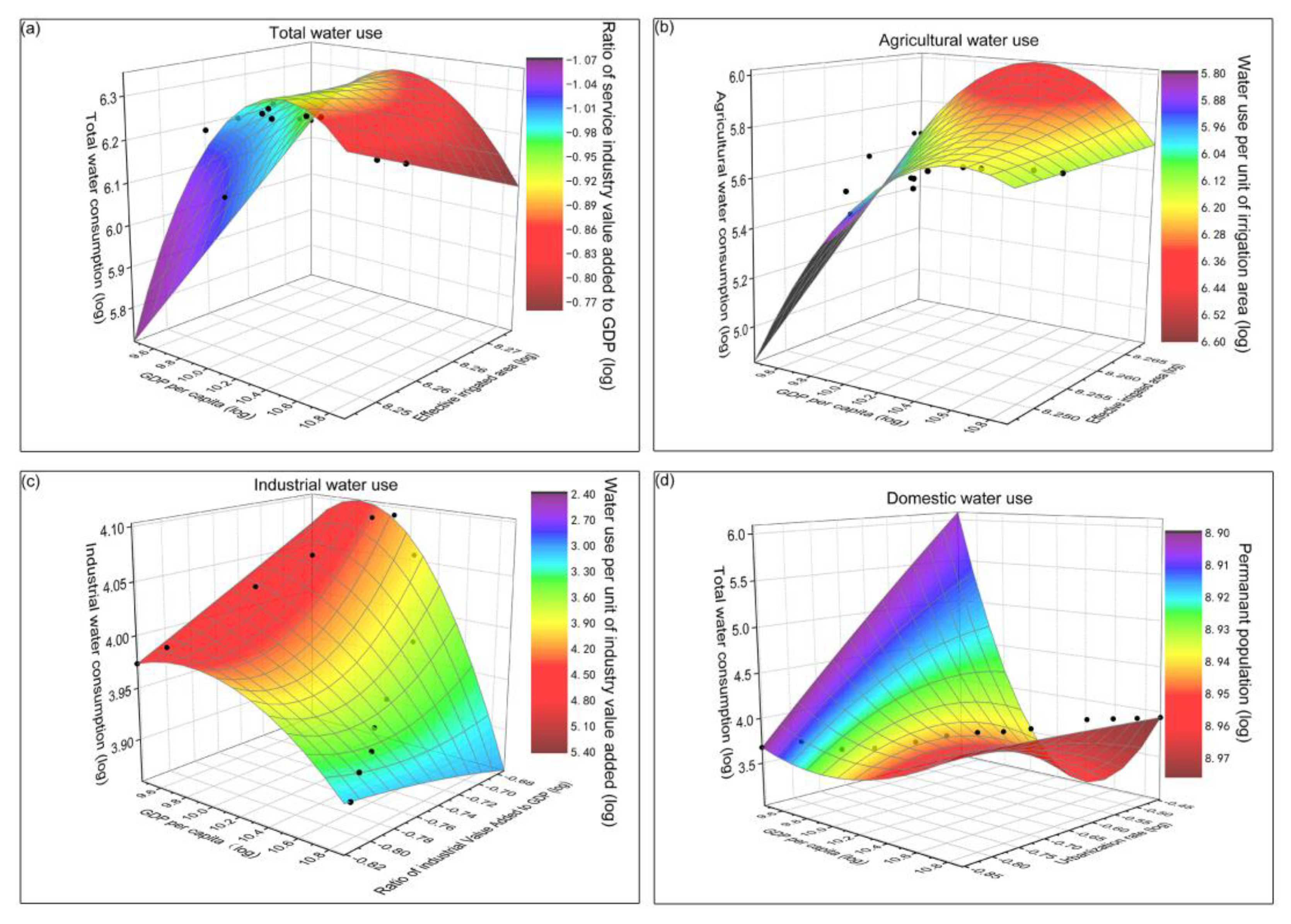
3.1. EKC Characteristics of Total Water Use and Different Industrial Water Uses

In order to judge whether the discussed environmental indicators had an inverted U-shape or not, multidimensional surface and scatter diagrams of the main explanatory variable were plotted for each type of water use. These diagrams help to intuitively express the EKC characteristics. If the type of water use conforms to inverted U-shaped characteristics, the quadratic logarithmic curve EKC model can be used to analyze its trend. If not, the cubic logarithmic curve EKC model will be used. Figure 2 shows the comprehensive multidimensional surface and scatter diagrams of total water use, agricultural water use, industrial water use, domestic water use, and their explanatory variables in the study area from 2005 to 2017.

The industrial water use in Jiangsu Province increased and then decreased (Figure 2c), showing a typical inverted U-shaped characteristic. Thus, the multivariate quadratic logarithmic curve EKC model was selected. The total water use (Figure 2a) and agricultural water use (Figure 2b) changes increased and decreased slowly, and sometimes they fluctuated with irrigated area. With regard to domestic water use, domestic water use still maintained an upward trend when income level and population growth increased (Figure 2d). The EKC model of the cubic logarithmic curve was selected because it could accurately simulate the fluctuation characteristics of the total water use, agricultural water uses, and domestic water use.

With the quadratic or cubic EKC models determined by the change characteristics of different environmental indicators, the LIMDEP software was used to perform nonlinear regression simulation with the univariate and multivariate EKC models.

Table 3. Comparison of univariate and multivariate model simulation results for different types of water use in Jiangsu Province.

Environmental Variable	EKC Model	β0/Constant	β1/lnX	β2/(lnX)2	β3/(lnX)3	β4/lnY	β5/lnZ	R2	F-Statistic	AIC
Total water use (ET)	univariate	368.003 (1.82)	−109.602 (−1.84) *	11.039 (1.88) *	−0.370 (−1.92) *	-	-	0.745	8.78	−2.987
	multivariate	388.867 (1.81) *	−138.550 (−2.34) **	13.832 (2.44) **	−0.458 (−2.54) **	9.304 (2.25) **	−1.361 (−1.52)	0.834	7.04	−3.109
Agricultural water use (EA)	univariate	501.671 (1.74)	−145.935 (−1.71)	14.285 (1.71)	−0.465 (−1.70)	-	-	0.512	3.15	−2.281
	multivariate	85.402 (4.43) ***	−27.453 (−5.24) ***	2.712 (5.29) ***	−0.089 (−5.33) ***	0.891 (50.50) ***	0.879 (1.72) *	0.997	659.98	−7.413
Industrial water use (EI)	univariate	−18.327 (−3.13) **	4.485 (3.89) ***	−0.225 (−3.97) ***	-	-	-	0.758	15.64	−3.558
	multivariate	−3.393 (−0.56)	−0.898 (−0.08)	0.052 (1.07)	-	0.714 (3.96) ***	0.860 (9.64) ***	0.988	169.91	−6.286
Domestic water use (EH)	univariate	447.819 (3.66) ***	−130.754 (−3.61) ***	12.796 (3.59) ***	−0.416 (−3.57) ***	-	-	0.953	60.64	−3.989
	multivariate	−692.948 (−1.80) *	108.876 (1.33)	−11.438 (−1.38)	0.393 (1.42)	−1.438 (−2.76) ***	39.988 (2.98) ***	0.973	50.30	−4.236

Note: The values in brackets are t-test statistics; the F-test statistics of the univariate model and the multivariate model at a significance level of 0.05 are 4.35 and 5.05, respectively; * represents significant at a significance level of 0.1; ** means significant at a level of 0.05; and *** means significant at a significance level of 0.01.

shows the results.

As shown in Table 3, the multivariate logarithmic curve model outperformed the univariate model in terms of the simulation results of total water use in the process of economic and social development, and the determination coefficient R² reached 0.834. This indicated that the proportion of the service industry in GDP, a newly added independent variable, had a negative coefficient.

Although the agricultural water use fluctuated partly in the process of economic and social development, it generally conformed to the inverted “U” pattern. The multivariate cubic logarithmic curve model produced better simulation results of agricultural water use than the univariate model. According to the t-test significance level of newly added independent variables, the influence of per capita income on agricultural water use was gradually weakened with the development of the economy and society. In contrast, the effects of effective irrigation area and science and technology on agricultural water use were significantly enhanced.

The simulation results of industrial water use showed that the improved multivariable quadratic logarithmic curve model outperformed the univariate model. With the development of the economy and society, per capita income was no longer the main factor affecting the change in industrial water use, and the role of industrial structure adjustment and science and technology was gradually enhanced.

The domestic water use did not show complete change characteristics of an inverted U-shape that first increased and then decreased. Due to the complex effects of multiple factors, such as the continuous population growth, the gradual increase in the quota of domestic water, and the application of water-saving technology and equipment at this stage, it was difficult to determine whether domestic water use conformed to the characteristics of an inverted U-shape. With regard to the simulation of domestic water use, the multivariable cubic logarithm curve model was not superior to the quadratic logarithm curve model, and even the positive and negative coefficients of some new independent variables were contrary to the practical significance. The main reason was that the complete inverted U-shaped change was characterized by rapid growth, followed by slow growth, and finally a decline. According to the data from 2005 to 2017, domestic water use in Jiangsu Province was in a continuous growth state. In addition, the limitation of data series also affected the simulation results of domestic water use.

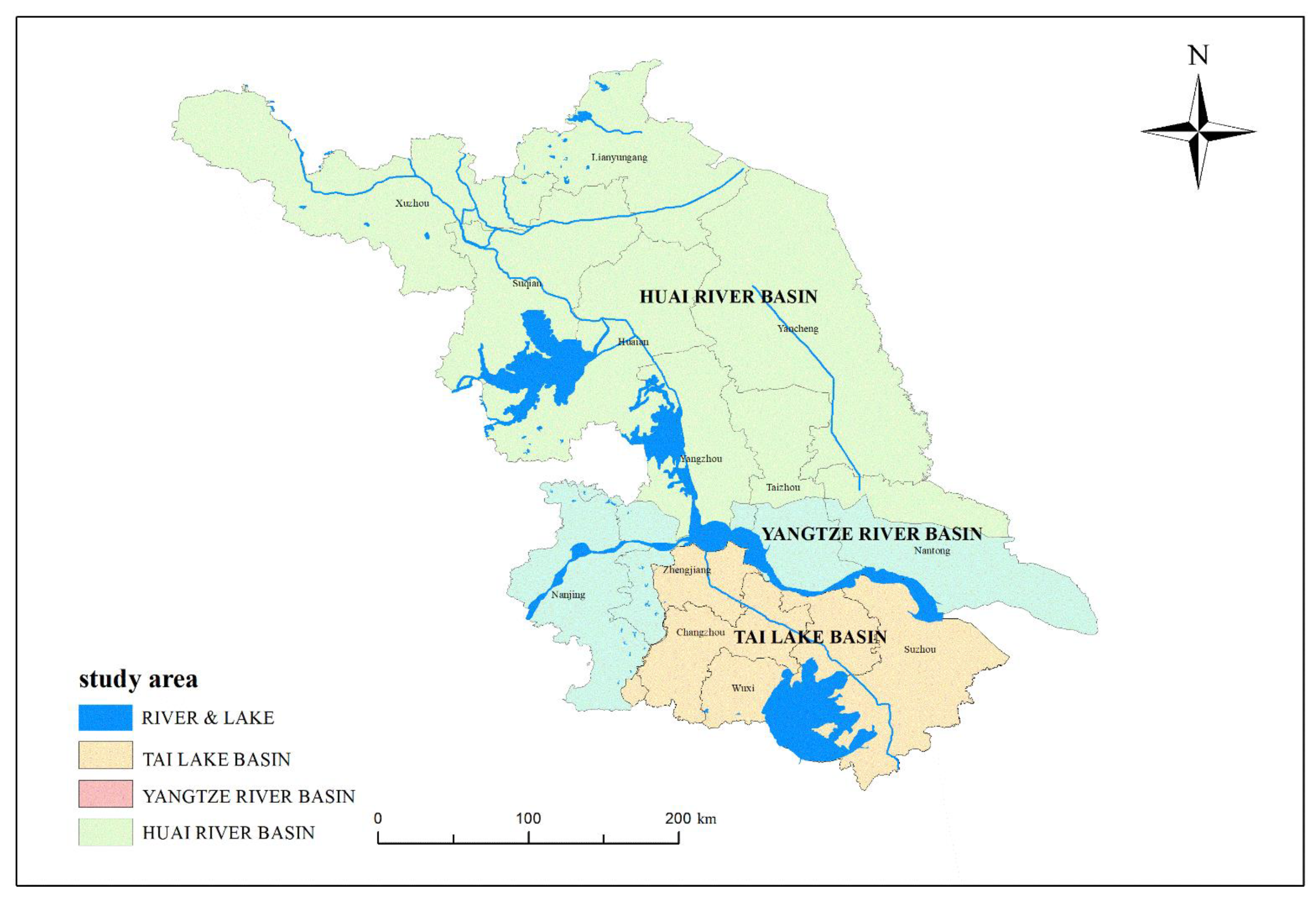
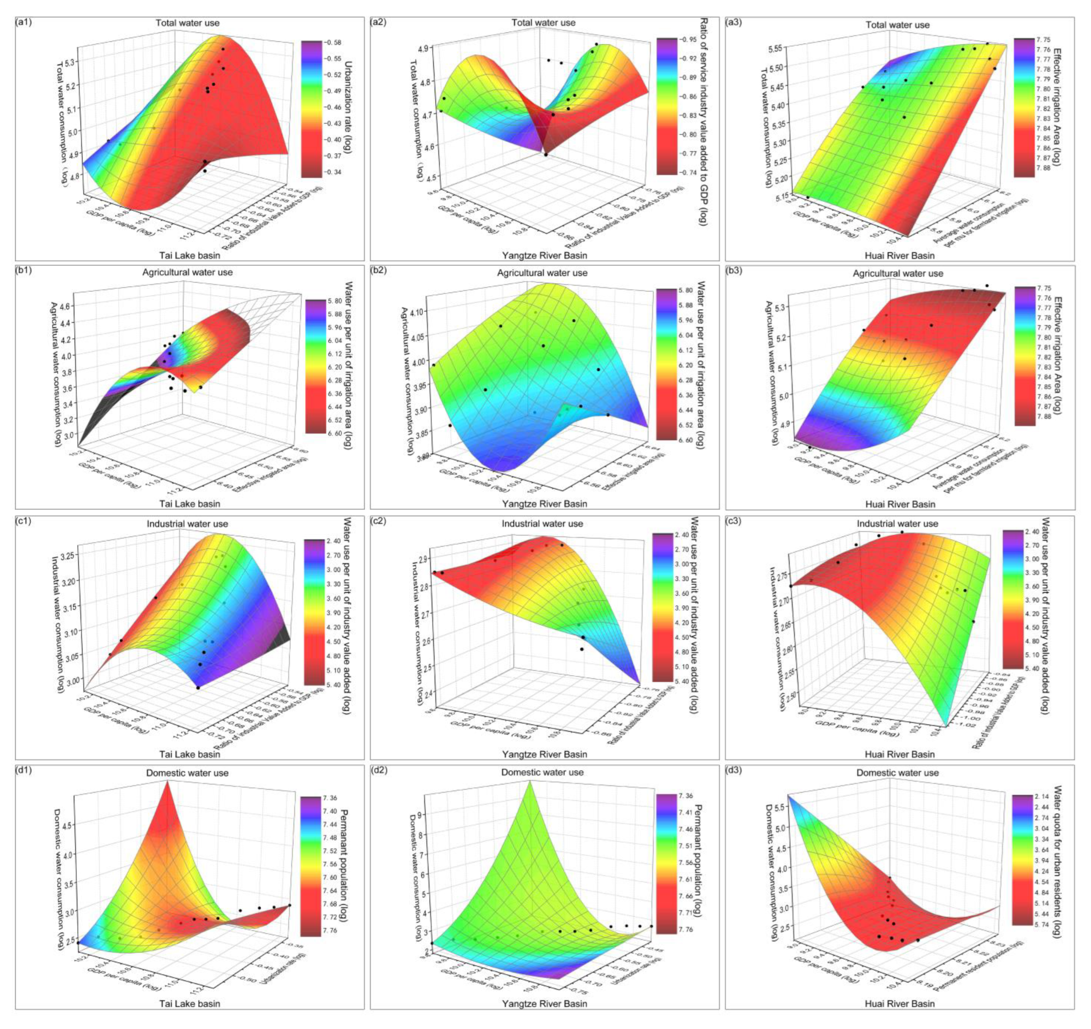
3.2. EKC Characteristics of Water Use in Different Regions of Jiangsu

In order to compare the EKC characteristics of total water use of three different river basins in Jiangsu Province, the EKC characteristics of the total water use and agricultural, industrial, and domestic water uses of the Tai Lake, Yangtze River, and Huai River basins were compared and analyzed. Similarly, in order to explain the significant effects of newly added independent variables on the total water use and the simulation effect of the multivariate model, multi-dimensional surface and scatter diagrams of the total water use and its main factors were plotted (Figure 3).

As shown in Figure 3, the total water use in the Tai Lake and Yangtze River Basins increased first and then decreased in a U-shaped pattern. The total water use in the Huai River Basin shifted from a long-term slow growth to a decline, showing a non-inverted U-shape. According to the curvature of the surface and the color change of the legend, the effects of the main factors on the total water use of each watershed could be concluded. Therefore, the quadratic logarithm curve model was selected as the total water use EKC model in the Tai Lake and Yangtze River Basins, while the cubic logarithm curve model was selected in the Huai River Basin and Jiangsu Province. The two most significant factors affecting the total water use change in each watershed were selected to construct a multivariate quadratic logarithmic curve model and a cubic logarithmic curve model, and the LIMDEP software was used to perform nonlinear regression simulations with the multivariate EKC measurement model. The initial value of each parameter was set as 1.

Table 4. Simulation results of univariate and multivariate models of total water use in three basins of Jiangsu Province.

Area	Model	β0/Constant	β1/lnX	β2/(lnX)2	β3/lnX3	β4/lnY	β5/lnZ	R2	F-Statistic	AIC
Tai Lake in Jiangsu Province	Single variable	−111.41 (−5.93) **	21.72 (6.17) ***	−1.01 (−6.13) ***	-	-	-	0.813	21.81	−2.266
	Multiple variables	−92.88 (−2.01) **	18.07 (2.09) **	−0.83 (−2.04) **	-	0.37 (0.45)	−0.72 (−0.44)	0.818	9.01	−1.985
Yangtze River Basin in Jiangsu Province	Single variable	−24.42 (−3.36) ***	5.68 (4.02) ***	−0.276 (−4.02) ***	-	-	-	0.62	8.09	−3.30
	Multiple variables	−2.35 (−0.11)	1.93 (0.47)	−0.98 (−0.50)	-	1.64 (1.53) *	1.10 (1.18) *	0.68	4.21	−3.36
Huai River in Jiangsu Province	Single variable	353.09 (1.55)	108.05 (−1.52)	11.16 (1.52)	−0.38 (−1.52)	-	-	0.556	3.76	−1.98
	Multiple variables	−115.70 (−3.40) ***	33.45 (3.27) ***	−3.42 (−3.23) ***	0.116 (3.19) ***	0.99 (3.19) ***	0.73 (25.99) ***	0.992	166.37	−5.65

Note: Values in brackets are t-test statistics; the F-test statistics of the univariate model and the multivariate model at a significance level of 0.05 are 4.35 and 5.05, respectively; * represents significant at a significance level of 0.1; ** means significant at a significant level of 0.05; *** means significant at a significance level of 0.001.

shows the results. In the process of economic and social development, the total water use of the Tai Lake and Yangtze River Basins exhibited typical inverted U characteristics, while the total water use of the Huai River Basin and Jiangsu Province was now in a stage of an inverted U-type (from an increasing trend to a decreasing trend). The multivariate quadratic and cubic logarithmic curve models were superior to the univariate model in total water use simulations. Although the coefficients of some newly added independent variables in the simulation results were negative, they were consistent with the practical significance. Although the urbanization rate of the Tai Lake Basin increased, the proportion of domestic water use in total water continued to decline from 8.73% in 2006 to 6.68% in 2008, and then it slowly increased, reaching 12.02% in 2017. This was contrary to the trend of total water use that increased first and then decreased. Thus, the urbanization rate coefficient in the simulation results was negative. The proportion of the added value of tertiary industry in GDP in Jiangsu Province increased annually at an average annual growth rate of 1.4%, was 37.88% in 2005, and reached 44.90% in 2017. Due to the low water use and higher water efficiency of tertiary industry compared to agriculture and industry, the proportion coefficient of the added value of tertiary industry in GDP was negative, which agreed with the practical significance.

4. Discussion

4.1. EKC Model and Its Uncertainty

Generally, simplified univariate quadratic and cubic curve models are used in EKC studies. Given that simplified univariate EKC models consider the economic development level as the only factor influencing water consumption, they ignore the actual complex relationship between water resources and economic society. Moreover, when the simplified model is used in different regions, there is a hypothesis that the economic development model between different regions and its impact on water consumption are basically the same. It makes the simulation results of EKC characteristics highly uncertain. In fact, the explanatory variables influencing water consumption change dynamically, especially in developing countries. Therefore, this study used the weighted grey absolute correlation analysis method to develop a multivariate EKC model, and this model was used to identify the main factors. This model outperformed the univariate model in terms of the simulation results. However, due to the complex relationship between water resources and economic society, the multivariate EKC model has some uncertainties in accurately describing the trend of water consumption [37,38], such as the selection of explanatory variables and year-on-year GDP conversion. Therefore, it is necessary to construct a comprehensive index to characterize the factors of water consumption change to increase the accuracy of model simulation results.

In addition, the multivariate EKC model is mainly used to describe the characteristics of water consumption increase or the trend from an increase to a decrease in the process of economic and social development. That means it can be used to simulate and verify whether the relationship between water resources and economic society agrees with an inverted “U”, but it is difficult to accurately simulate the characteristics of water consumption change from a decline to a stable stage. It is also difficult to predict the balance point of per capita income and water consumption turning from a declining phase to a stable phase. This will the focus of future research.

4.2. EKC Characteristic Simulation and Its Uncertainty in Jiangsu Province

According to the results of EKC characteristics of different industrial water uses and the results in three watershed regions in Jiangsu Province, the effects of the main factors on the total water use of each watershed could be concluded as follows. First, the ratio of industrial added value to GDP in the Tai Lake Basin and the Yangtze River Basin played a major role in controlling the total water use, and the total water use increased first and then decreased with the ratio of industrial added value to GDP. The urbanization rate of the Tai Lake Basin was significantly higher than those of the other two basins, and it has increased steadily, effectively promoting increases in domestic water uses and playing an important role in the change in total water use. Although the proportion of the added value of tertiary industry in the GDP of the Yangtze River Basin was less than the proportion of the industrial added value to the GDP, it played an important role in restraining the increase of the total water use in the basin. This phenomenon was also found in Turkey [14].

The results also can be discussed according to the actual data on GDP growth, such as the relationship between domestic water use and economic growth. According to the simulation results, it did not present inverted U-shaped change characteristics. In fact, the service industry in Jiangsu Province accounted for 37.88% of its GDP in 2005, and it increased to 44.90% in 2017, with an annual growth rate of 1.4%. The total water uses of tertiary industry were less than those of agriculture and industry, and the water use efficiency was higher than those of agriculture and industry. Therefore, the ratio coefficient of the added value of tertiary industry to GDP did not represent an inverted U shape, which agreed with practical significance [15,39].

Furthermore, studies on the relationship between water use and per capita income with the EKC model require the support of long series data of socio-economic and water resources’ development and utilization. Due to limited data conditions, the relationships in other cases were not analyzed. Fortunately, Jiangsu Province is a developed region with a developed social economy in China. The EKC model could be more suitable to be used in this study than other regions in China. In any case, there are still some uncertainties in this study. In order to reduce these uncertainties, the balance relationships in other similar regions, such as the Pearl River Delta region of China, will be analyzed and compared in the future.

5. Conclusions and Policy Implications

5.1. Conclusions

In order to describe the balance relationship between water use and per capita income in Jiangsu Province, this study developed a multivariable EKC model with the grey absolute correlation method. The water use was divided into four categories: regional total water use, industrial water use, agricultural water use, and domestic water use. The relationships between different categories of water use and per capita income were simulated in three sub-regions (the Tai Lake, Yangtze River, and Huai River Basins). According to the results of EKC characteristics in Jiangsu Province, the main conclusions are as follows:

(1)

The improved multivariable EKC model was suitable to describe the inverted U-shaped change characteristics of water use, and it outperformed the univariate EKC model in simulating industrial water use, agricultural water use, and total water use in the study area. According to the trends of different water uses in the three basins of Jiangsu Province, adaptation measures for water use change in different sections in these basins were proposed, such as adjusting industrial structure, strengthening rational agricultural water use, scientifically strengthening industrial and domestic water uses, and promoting water-saving technology.

(2)

The improved weighted grey absolute correlation analysis method rationally and quantitatively evaluated the factors controlling water consumption. The main factors of different water uses were distinct in the three sub-regions in Jiangsu Province. In the three sub-regions, the predominant factor of industrial water consumption was industrial added value proportion in GDP, followed by water use per unit of industrial added value. For agricultural water consumption, the factors were the irrigated area and water use per unit of irrigation area, and the three sub-regions exhibited differences in the primary and secondary roles of these factors due to different agricultural development conditions. For domestic water consumption, the main factor in the Tai Lake and the Yangtze River Basins was the urbanization rate, followed by the permanent population. In contrast, the primary and secondary factors in the Huai River Basin were permanent population and water quotas for urban residents. The factors controlling total water consumption in the three sub-regions were different. In the case of the Tai Lake Basin, the primary and secondary factors were the proportion of industrial added value to GDP and urbanization rate, respectively. Those in the Yangtze River Basin were industrial added value in proportion to GDP and service industry added value proportion to GDP, and the irrigated area and service industry added value proportion in GDP were the dominant factors in the Huai River Basin.

(3)

The EKC curve of economic growth and water resources impacts was not the common development model in Jiangsu Province. The balanced relationship between economic growth and water resource utilization presented different characteristics in the process of economic and social development. Different water use categories had various EKC features in different regions. Industrial water use agreed with the characteristics of a significant inverted U-shaped change, and it was currently in the inverted decline stage of the U curve. Agricultural water uses also agreed with the EKC characteristics of the inverted U-shaped curve. At present, the agricultural water uses in the Tai Lake Basin were in the decreasing stage of the inverted U curve. The Yangtze River Basin was in the transitional stage of the inverted “U” from an increasing trend to a decreasing trend. The water uses in the Huai River Basin and Jiangsu Province were just in the increasing stage. The change of total water uses also agreed with the characteristics of the inverted U curve. The water uses in the Tai Lake and Yangtze River Basins were in the declining stage of the inverted U curve, and that in the Huai River Basin of Jiangsu Province had just entered the decline stage. However, the domestic water use showed an upward trend from 2005 to 2017. Thus, it was impossible to determine whether domestic water use conforms to the inverted U-shaped change characteristics.

5.2. Policy Implications

With the economic and social development, different sections in various river basins of Jiangsu Province needed to take further measures to ensure the coordinated and sustainable development of water resources, the economy, and the ecological environment.

The government shall adjust the industrial structure. Industrial structure adjustment was an important support to achieve the transformation of economic growth mode, reasonably allocate water resources, and promote the sustainable development of water resources. Although the three river basins in Jiangsu Province have different levels of economic development, their industrial structure adjustment steps are basically the same. The ratio of primary industry with high water use was decreasing, while that of tertiary industry with low water use was increasing. The agricultural water use in the Huai River Basin was transiting from an increasing trend to a decreasing trend. It is necessary to further optimize the industrial structure, vigorously develop secondary and tertiary industries, and promote total water use to rapidly enter the declining stage of the inverted U-shape. As for the Tai Lake and Yangtze River basins, it is necessary to increase the proportion of tertiary industry in order to control the total amount of water use and to reach the stable stage of the inverted U-shape as soon as possible.

As for water users, the first measure is to strengthen rational water use in agriculture. Although non-agricultural water use in Jiangsu Province has increased annually, agriculture, as a major water user, still comprises a large proportion of water use. According to the characteristics of the EKC simulation, the Huai River Basin had the largest agricultural water-saving potential, followed by the Yangtze River and Tai Lake Basins. The agricultural output value of the Huai River Basin accounted for a higher proportion of the regional GDP. Thus, improvement of the agricultural water use efficiency is a key measure to promote agricultural water use to enter a continuous decline stage. For water users, the second measure is to strengthen scientific water use in the industrial and domestic sections. Although the industrial water use efficiency has increased in Jiangsu Province, the water use per unit of industrial added value was significantly different in the three sub-regions. Therefore, it is necessary to adjust the industrial structure and industrial layout, especially in the Yangtze River and Huai River Basins, in order to reach the stable stage of the industrial water pouring U curve as soon as possible.

With regard to the public, it is urgent to raise their awareness of water saving. Water saving is a work of a whole society, which requires the full participation of the government, enterprises, and individuals. In addition, it is necessary to vigorously promote the transformation of water-saving technologies based on science and technology and raise awareness of water saving in the whole of society. Especially, domestic water consumption is not a production activity but a consumption activity, so water consumption tends to increase with the improvement of living standards. Therefore, water saving becomes a public good that depends on the conscious behavior of the public, which requires the full participation of the government, enterprises and individuals. The key measures to promote the decrease of domestic water consumption in the future are to promote the publicity of green life, popularize water-saving instruments, and adjust water consumption behavior with water price. Therefore, once domestic water consumption decreases with the improvement of the social development level, it is precisely a sign that social development has reached a new level of developed areas not only in material growth but also in cultural prosperity. From this point of view, the EKC curve not only reflects the impact of GDP growth on the natural environment, but also reflects the impact of social civilization degree on the natural environment.

With the aforementioned efforts, a harmonious relationship between water and socio-economic development is expected to be established, and sustainable utilization of water resources can be achieved to ensure sustainable social and economic development.

References

1. Fan, Y.; Park, S.; Nan, Z. Participatory Water Management and Adoption of Micro-Irrigation Systems: Smallholder Farmers in Arid North-Western China. Int. J. Water Resour. Dev. 2018, 34, 434–452. [Google Scholar] [CrossRef]
2. Liu, Y.; Zhang, Z.; Zhang, F. Challenges for Water Security and Sustainable Socio-Economic Development: A Case Study of Industrial, Domestic Water Use and Pollution Management in Shandong, China. Water 2019, 11, 1630. [Google Scholar] [CrossRef] [Green Version]
3. Esen, Ö.; Yıldırım, D.Ç.; Yıldırım, S. Threshold Effects of Economic Growth on Water Stress in the Eurozone. Environ. Sci. Pollut. Res. 2020, 27, 31427–31438. [Google Scholar] [CrossRef]
4. Duarte, R.; Pinilla, V.; Serrano, A. Is There an Environmental Kuznets Curve for Water Use? A Panel Smooth Transition Regression Approach. Econ. Model. 2013, 31, 518–527. [Google Scholar] [CrossRef] [Green Version]
5. Stern, D.I. The Rise and Fall of the Environmental Kuznets Curve. World Dev. 2004, 32, 1419–1439. [Google Scholar] [CrossRef]
6. Orubu, C.O.; Omotor, D.G. Environmental Quality and Economic Growth: Searching for Environmental Kuznets Curves for Air and Water Pollutants in Africa. Energy Policy 2011, 39, 4178–4188. [Google Scholar] [CrossRef]
7. Ji, S.C.; He, H.; Wu, Z.Y. Progress in Application of Environmental Kuznets Curve to Water Resources Field. Water Resour. Prot. 2015, 30, 1–6. (In Chinese) [Google Scholar] [CrossRef]
8. Sun, S.; Bao, C.; Fang, C.L. Freshwater Use in China: Relations to Economic Development and Natural Water Resources Availability. Int. J. Water Resour. Dev. 2020, 36, 738–756. [Google Scholar] [CrossRef]
9. Guo, W.; Asghar, N.; Ahmad, I.; Yin, W.; Abbas, Q.; ur Rahman, S.; Farooq, F. Economic Growth, Fiscal Imbalance, and Environmental Sustainability: What Is Desirable and Undesirable for Developing Economies? Environ. Sci. Pollut. Res. 2021, 28, 52283–52294. [Google Scholar] [CrossRef]
10. Kuznets, S. Economic Growth and Income Inequality. Am. Econ. Rev. 1955, 45, 1–28. [Google Scholar]
11. Grossman, G.M.; Krueger, A.B. Environmental Impacts of a North-American Free-Trade Agreement. In The U.S. Mexico Free Trade Agreement; Garber, P.M., Ed.; MIT Press: Cambridge, MA, USA, 1993; pp. 13–56. [Google Scholar]
12. Kaika, D.; Zervas, E. The Environmental Kuznets Curve (EKC) Theory—Part A: Concept, Causes and the CO2 Emissions Case. Energy Policy 2013, 62, 1392–1402. [Google Scholar] [CrossRef]
13. Karahasan, B.C.; Pinar, M. The Environmental Kuznets Curve for Turkish Provinces: A Spatial Panel Data Approach. Environ. Sci. Pollut. Res. 2022, 29, 25519–25531. [Google Scholar] [CrossRef] [PubMed]
14. Tirgil, A.; Acar, Y.; Ozgur, O. Revisiting the Environmental Kuznets Curve: Evidence from Turkey. Environ. Dev. Sustain. 2021, 23, 14585–14604. [Google Scholar] [CrossRef]
15. Rao, C.; Yan, B. Study on the Interactive Influence between Economic Growth and Environmental Pollution. Environ. Sci. Pollut. Res. 2020, 27, 39442–39465. [Google Scholar] [CrossRef] [PubMed]
16. Pandit, M.; Paudel, K.P. Water Pollution and Income Relationships: A Seemingly Unrelated Partially Linear Analysis. Water Resour. Res. 2016, 52, 7668–7689. [Google Scholar] [CrossRef]
17. Liu, S.J.; Li, J.; Xu, X.L. Pollution Emissions and Economic Growth Revisited: A Novel Model of Spatial Hyperbolic Decomposition in Sewage Reduction Risk Management. Water Resour. Res. 2022, 58, e2021WR030746. [Google Scholar] [CrossRef]
18. Sun, S.; Fang, C. Water Use Trend Analysis: A Non-Parametric Method for the Environmental Kuznets Curve Detection. J. Clean. Prod. 2018, 172, 497–507. [Google Scholar] [CrossRef]
19. Song, Z.; Jia, S. Municipal Water Use Kuznets Curve. Water Resour. Manag. 2022, preprint. [Google Scholar] [CrossRef]
20. Expósito, A.; Pablo-Romero, M.; Sánchez-Braza, A. Testing EKC for Urban Water Use: Empirical Evidence at River Basin Scale from the Guadalquivir River, Spain. J. Water Resour. Plan. Manag. 2019, 145, 04019005. [Google Scholar] [CrossRef]
21. Lu, W.C. Industrial Water Use, Income, Trade, and Employment: Environmental Kuznets Curve Evidence from 17 Taiwanese Manufacturing Industries. Environ. Sci. Pollut. Res. 2018, 25, 26903–26915. [Google Scholar] [CrossRef]
22. Zhang, H.; Long, Z.; Zhang, C. When Will China’s Total Water Consumption Reach the Turning Point? EKC Simulation and Influencing Factors. Environ. Sci. Pollut. Res. 2022, ahead of print. [Google Scholar] [CrossRef]
23. Hosseinzadeh, M.; Saghaian, S.H.; Nematollahi, Z.; Shahnoushi Foroushani, N. Water Consumption and Economic Growth: Evidence for the Environmental Kuznets Curve. Water Int. 2022, 1–16. [Google Scholar] [CrossRef]
24. Sebri, M. Testing the Environmental Kuznets Curve Hypothesis for Water Footprint Indicator: A Cross-Sectional Study. J. Environ. Plan. Manag. 2016, 59, 1933–1956. [Google Scholar] [CrossRef]
25. Rashid Gill, A.; Viswanathan, K.K.; Hassan, S. The Environmental Kuznets Curve (EKC) and the Environmental Problem of the Day. Renew. Sustain. Energy Rev. 2018, 81, 1636–1642. [Google Scholar] [CrossRef]
26. Katz, D.L. Water, Economic Growth, and Conflict: Three Studies. Ph.D. Thesis, University of Michigan, Ann Arbor, MI, USA, 2008. [Google Scholar]
27. Cole, M.A. Economic Growth and Water Use. Appl. Econ. Lett. 2004, 11, 1–4. [Google Scholar] [CrossRef]
28. Jia, S.; Yang, H.; Zhang, S.; Wang, L.; Xia, J. Industrial Water Use Kuznets Curve: Evidence from Industrialized Countries and Implications for Developing Countries. J. Water Resour. Plan. Manag. 2006, 132, 183–191. [Google Scholar] [CrossRef] [Green Version]
29. Goklany, I.M. Comparing 20th Century Trends in U.S. and Global Agricultural Water and Land Use. Water Int. 2002, 27, 321–329. [Google Scholar] [CrossRef]
30. Richard, J. Culas Deforestation and the Environmental Kuznets Curve: An Institutional Perspective. Ecol. Econ. 2007, 61, 429–437. [Google Scholar] [CrossRef]
31. Yang, W.P.; Yuan, X.L. Hypothesis of environmental Kuznets curve and its test in China. Resour. Environ. Yangtze Basin 2009, 18, 704–710. (In Chinese) [Google Scholar]
32. Baek, J. Environmental Kuznets Curve for CO2 Emissions: The Case of Arctic Countries. Energy Econ. 2015, 50, 13–17. [Google Scholar] [CrossRef]
33. Li, T.T.; Wang, Y.; Zhao, D.T. Environmental Kuznets Curve in China: New Evidence from Dynamic Panel Analysis. Energy Policy 2016, 91, 138–147. [Google Scholar] [CrossRef]
34. Xu, T. Investigating Environmental Kuznets Curve in China-Aggregation bias and policy implications. Energy Policy 2018, 114, 315–322. [Google Scholar] [CrossRef]
35. Thomas, M.; Daqing, S. Environmental Quality and Development: Is There a Kuznets Curve for Air Pollution Emissions? J. Environ. Econ. Manag. 1994, 27, 147–162. [Google Scholar] [CrossRef]
36. Grossman, G.M.; Krueger, A.B. Economic Growth and the Environment. Q. J. Econ. 1995, 110, 353–377. [Google Scholar] [CrossRef] [Green Version]
37. Hao, Y.; Hu, X.L.; Chen, H.Y. On the relationship between water use and economic growth in China: New evidence from simultaneous equation model analysis. J. Clean. Prod. 2019, 235, 953–965. [Google Scholar] [CrossRef]
38. Wang, Z.B.; Bu, C.; Li, H.M.; Wei, W.D. Seawater environmental Kuznets curve: Evidence from seawater quality in China’s coastal waters. J. Clean. Prod. 2019, 219, 925–935. [Google Scholar] [CrossRef]
39. Wang, J.F.; Feng, S.Q.; Pang, D.Y.; Zhou, Y.; Liu, M.Y. Mixing data modelling method for response of water environment quality to economic development. IOP Conf. Ser. Earth Environ. Sci. 2019, 227, 052024. [Google Scholar] [CrossRef]
Figure 1. Three sub-regions (watershed zoning) of Jiangsu Province.
Sustainability 14 16851 g001
Figure 2. Relationship between water use in different categories and its main factors. ((a) Total water use; (b) Agricultural water use; (c) Industrial water use; (d) Domestic water use).
Sustainability 14 16851 g002
Figure 3. Relationship between total water use and main influencing factors in the three basins in Jiangsu Province (a1d1:Tai Lake Basin; a2d2:Yangtze River Basin; a3d3: Huai River Basin).
Sustainability 14 16851 g003