Gaussian Process Regression Based Multi-Objective Bayesian Optimization for Power System Design

Abstract

Within a disruptively changing environment, design of power systems becomes a complex task. Meeting multi-criteria requirements with increasing degrees of freedom in design and simultaneously decreasing technical expertise strengthens the need for multi-objective optimization (MOO) making use of algorithms and virtual prototyping. In this context, we present Gaussian Process Regression based Multi-Objective Bayesian Optimization (GPR-MOBO) with special emphasis on its profound theoretical background. A detailed mathematical framework is provided to derive a GPR-MOBO computer implementable algorithm. We quantify GPR-MOBO effectiveness and efficiency by hypervolume and the number of required computationally expensive simulations to identify Pareto-optimal design solutions, respectively. For validation purposes, we benchmark our GPR-MOBO implementation based on a mathematical test function with analytically known Pareto front and compare results to those of well-known algorithms NSGA-II and pure Latin Hyper Cube Sampling. To rule out effects of randomness, we include statistical evaluations. GPR-MOBO turnes out as an effective and efficient approach with superior character versus state-of-the art approaches and increasing value-add when simulations are computationally expensive and the number of design degrees of freedom is high. Finally, we provide an example of GPR-MOBO based power system design and optimization that demonstrates both the methodology itself and its performance benefits.

1. Design of Complex Power Systems

Design of power systems is facing a triple disruptive upheaval: (i) primary energy sources are being converted from fossil to renewable, (ii) grid topologies are moving from centralized to decentralized dominance, and (iii) previously separate sectors (heat, electricity, and mobility) are merging. Driven by these changes, emerging technologies will replace established ones, while at the same time the number of degrees of freedom in facility design will increase. The resulting VUCA (volatile, uncertain, complex and ambiguous) [1] environment poses significant risks for all involved stakeholders throughout the value chain, from product owners over system architects to operators and consumers. Simultaneous ecologic and economic success of power plants requires the ability to identify system design alternatives with multi-objective optima in terms of cost-benefit trade-off for individual use cases.

The lack of technical experience around emerging or new technologies significantly increases the challenge of optimization. Virtual prototyping (VP) guided by engineering experience, therefore, may be considered the standard approach for today’s energy facility design. However, with an increasing number of technology alternatives and decreasing system-level technical experience, the dependence between objectives and design parameters is unknown in many cases. Power system design, thereby, becomes a black box multi-objective optimization (MOO) problem.

VP-based MOO guided by engineering intuition again fails when engineering experience is lacking and full or fractional factorial coverage of the design space is not a viable option due to (i) the dimensionality (i.e., number of degrees of freedom) of the design space and (ii) the time-consuming and costly effort required to simulate power systems. Therefore, gaining engineering knowledge about the relationship between system design objectives as a function of design parameters based on as few simulations as possible is of paramount importance.

VUCA driven power system design, accordingly, requires MOO algorithms being

(i)

effective, i.e., knowledgable of multi-objective (MO) related optimal cost-benefit (lateron called Pareto-optimal) trade-offs and

(ii)

efficient, i.e., requiring only a limited number of required (computationally expensive) simulations for quantifying these trade-offs.

While a broad variety of MOO approaches in black box environments deals with effective algorithms, only few of them meet the efficiency criterion [2]. Specifically Bayesian Optimization (BO) [3,4,5,6] algorithms based on Gaussian Process Regression (GPR) [3,7,8,9] appear as interesting effective and efficient MOO candidates.

GPR [10,11] provides a regression model that (in contrast to alternative methodical approaches) (a) does not suffer from the “curse of dimensionality” [12] ([Section 3.1]), and (b) inherently provides a quantification of regression uncertainty of the model. This uncertainty is exploited by the BO approach [13] which in turn is used to optimize the surrogate. For a more detailed and fundamental comparison of MOO approaches, we recommend [14].

In this paper, we present the mathematical background of GPR-based Bayesian Optimization (GPR-MOBO) in detail. This includes statements and selected proofs of key results. With that theoretical foundation on hand, we derive a computer implementation of an introduced GPR-MOBO algorithm, quantify its effectiveness and efficiency, and demonstrate the superiority of GPR-MOBO over state-of-the-art MOO algorithms, including a GPR-MOBO application to a power system design example. The paper is structured as follows: Section 2 restates the introductory problem in mathematical terms, including definitions such as “Pareto-optimality” or “hypervolume”. Section 3 explains Gaussian Process Regression (GPR) and a Bayesian Optimization (BO) based on it before a bipartite validation follows in Section 4: First, the superiority of the presented approach is validated via a mathematical test function before the proposed GPR-MOBO approach is applied to the design and optimization of a real life power system. Section 6 discusses our results, gives a brief summary and highlights ideas for future work.

2. Problem Statement in Mathematical Terms

Within this chapter, we phrase the task of effectively and efficiently identifying objective trade-offs in mathematical terms. For this purpose, we consider an (unknown) $t—$dimensional black box function

$$f:X\to {ℝ}^t.$$

We refer to $X\subset {ℝ}^d$ as the design space with target space ${ℝ}^t$ for $d,t\in \mathbb{N}$. Assume further, we can sample f at a finite number of points, i.e., choosing $x_1,\dots ,x_N$ we obtain $f\left(x_1\right),\dots ,f\left(x_N\right)$. We translate the MOO issue

$$d_{\mathrm{opt}}=\underset{d\in X}{argmin}f\left(d\right)$$

of identifying an optimal design $d_{\mathrm{opt}}\in X$ to finding solutions of f which represent non-dominated (Pareto-optimal) trade-offs of f, i.e., we are looking for Pareto points of f:

Definition 1 (Pareto point and front).

We write

$$\begin{array}{ccc}\hfill t\preccurlyeq s& :⟺& \forall i:t_i\le s_i\hfill \\ \hfill t\prec s& :⟺& \forall i:t_i<s_i.\hfill \end{array}$$

Then, given a set $S\subset {ℝ}^t$, a point $s\in S$ is called Pareto point, if there exists no other point $t\in S$ satisfying $t\preccurlyeq s$ and $t_i<s_i$ for some component i. The set of all Pareto (optimal) points is called the Pareto front of S.

More general, an $x\in X$ is a Pareto point of f if $f\left(x\right)$ is a Pareto point of $f\left(X\right)=\left\{f\right(x):x\in X\}$. The set of all such points is called Pareto front of f.

Based on this definition, we will call a MOO algorithm to be effective whenever it is capable to identify the set of non-dominated (Pareto-optimal) trade-offs for the (unknown) black box function. Introducing a measure of effectiveness, we will now define the so-called hypervolume.

Definition 2 (Hypervolume).

Denote by

$$I:{ℝ}^t\times {ℝ}^t\to \mathcal{P}\left({ℝ}^t\right),(x,r)\mapsto \{z\in {ℝ}^t:x\preccurlyeq z\prec r\}$$

the function sending two t-dimensional real vectors to the cube bounded by them where $\mathcal{P}$ denotes the power set. The Hypervolume of some (finite) set $Y\subset {ℝ}^t$ with respect to a reference point $r\in {ℝ}^t$ is given by the Lebesgue-measure

$${HV}_r\left(Y\right)={\lambda }_t\left({\bigcup }_{y\in Y}I(y,r)\right)$$

of the union over all cubes bounded by the reference point and by some point in Y.

Figure 1 illustrates the Hypervolume on exemplary base in two dimensions.

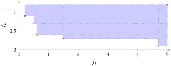
Figure 1. Hypervolume (blue area) in ${ℝ}^2$. The dotted rectangles illustrate the volumes i.e., $I(u,r)$ spanned by the respective point $u\in U$ (×) and the reference point r (×).

The Hypervolume is closely related to Pareto points in the following sense.

Proposition 1.

Let $S\subset {ℝ}^t$ be quasi-compact (i.e., bounded and closed) and $U\subset S$ be a finite subset. Let $r\in {ℝ}^t$ such that

$${HV}_r(U\cup \left\{s\right\})>{HV}_r\left(U\right)$$

for some $s\in S$. Then,

$$p^{\prime }=\underset{p\in S}{argmax}{HV}_r(U\cup \left\{p\right\})$$

is a Pareto point of S.

Proof. 

See Appendix A.  □

In simple words, Proposition 1 states that maximizing the hypervolume by adding an image (black box function) point implies this point to be a Pareto point. Accordingly, hypervolume is a suitable indicator of MOO effectiveness while the number of (simulation) samples required to find such Pareto points itself is a suitable measure for efficiency.

3. Bayesian Optimization Based on Gaussian Process Regression

Gaussian Process Regression (GPR) based Bayesian Optimization (BO) using Expected Hypervolume Improvement (EHVI, see Section 3.3) as acquisition function is a promising algorithmic approach to meet the simultaneous goals of effectiveness and efficiency. The following sub-sections will introduce the general mathematical GPR background (Section 3.1), choice of GPR related hyperparameters (Section 3.2) and GPR based multi-objective BO (GPR-MOBO, Section 3.3) prior summarizing previous sub-sections as a mathematical base for the subsequent algorithmic implementation.

3.1. Gaussian Process Regression

We summarize and recall the definition, statements and formulas needed in order to properly apply Gaussian Process Regression (GPR).

3.1.1. Multivariate Normal Distribution

Let $n\in \mathbb{N}$ be a positive integer and $C\in M_n(ℝ)$ be a real, positive definite matrix of dimension n with $M_n(ℝ)$ being the space of $n\times n$ matrices with values in ℝ. Let $m\in {ℝ}^n$ be a n-dimensional real vector. Recall the multivariate normal distribution $\mathcal{N}(m,C)$ to be the probability measure on ${ℝ}^n$ induced by the density function

$$f_{C,m}:{ℝ}^n\to ℝ,x\mapsto \frac{exp(-0.5{(x-m)}^{\top }{C}^{-1}(x-m))}{\sqrt{det\left(C\right){\left(2\pi \right)}^n}}.$$

The vector m is called mean(-vector) and the matrix C is called covariance matrix of $\mathcal{N}(m,C)$.

Multivariate normal distributions are stable under conditioning in the following sense.

Theorem 2.

Let $X_1,X_2$ be two random variables such that $(X_1,X_2)$ is multivariate normal $\mathcal{N}(m,C)$-distributed with mean $m=(m_1,m_2)\in {ℝ}^p\times {ℝ}^q$ and covariance matrix

$$C=\left[\begin{array}{cc}{C}_1& C_2\\ C_3& C_4\end{array}\right]\in M_{p+q}\left(\mathbb{R}\right),C_1\in M_p\left(\mathbb{R}\right).$$

Then, given some $x\in {ℝ}^q$ in the co-domain of $X_2$, the conditional density function of $X_1$ given $X_2=x$ is given by $f_{C^{\prime },m^{\prime }}$ with

$$m^{\prime }=m_1+C_2{C}_4^{-1}(x-m_2)$$

and

$$C^{\prime }=C_1-C_2{C}_4^{-1}{C}_3.$$

Proof. 

Theorem 2.5.1 in [15].  □

In particular, conditioning a multivariate normal distribution turns out to be multivariate normal distributed as well.

3.1.2. Stochastic Processes

Let $(\Omega ,\mathcal{F},P)$ be a probability space, I a set and $(S,{\mathcal{F}}^{\prime })$ be a measurable space.

Definition 3.

A stochastic process with state space S and index set I is a collection of random variables $X_i:\Omega \to S,i\in I$.

Remark 1.

Recall that arbitrary products of measurable spaces exist and their underlying sets are given by the Cartesian products of sets. By the universal property of the product, a stochastic process $X_i,i\in I$, therefore, consists of the same data as a measurable function $X:\Omega \to S^I$.

Given a stochastic process $X:\Omega \to S^I$, in practice, we are mostly interested in the induced measure $P_X=P\left(X^{-1}(-)\right)$ on $S^I$. On the other hand, given such probability measure $P_I$ on $S^I$, we obtain a stochastic process $p{r}_i:S^I\to S$ given by the canonical projections. In that sense, a stochastic process may be seen as a proper construction of a probability measure on the product space $S^I$.

3.1.3. Gaussian Process

With the definition of stochastic processes on hand, we can generalize the multivariate normal distribution (defined on finite products of real numbers) to possible infinite products of real numbers in the following sense.

Definition 4 (Gaussian Process).

Let X be a set. A Gaussian Process with index set X is a family of real valued random variables ${\left(r_x\right)}_{x\in X}$ such that for every finite subset $U\subset X$, the random variable ${\left(r_u\right)}_{u\in U}$ is multivariate normal distributed.

Recall that by the above, this induces a probability measure on ${ℝ}^I$. We can “construct” Gaussian Processes in the following way:

Theorem 3.

Let X be a set, $C:X\times X\to ℝ$ be a positive quadratic form in the sense that for every finite subset $U\subset X$ the induced matrix

$$C_U={\left(C(u_1,u_2)\right)}_{u_1,u_2\in U}$$

is positive definite and $m:X\to ℝ$ be a function. Given a subset $U\subset X$, denote by

$$m_U={\left(m\left(u\right)\right)}_{u\in U}$$

the induced vector.

Then, there exists a unique probability measure P on ${ℝ}^X$ satisfying

$$P_{p{r}_U}=P\circ p{r}_U^{-1}=\mathcal{N}(m_U,C_U)$$

for all $U\subset X$ finite where $p{r}_U:{ℝ}^X\to {ℝ}^U$ denotes the canonical projection.

The function C is called covariance function and m is called mean function of P.

Proof. 

See Appendix B.  □

In other words, we construct Gaussian Processes by choosing a positive quadratic form C further referred to as covariance function and a mean function m.

Example 4 (Squared exponential kernel).

The squared exponential kernel

$$\begin{array}{c}\hfill k_{l,{\sigma }_{\mathrm{c}}^2}:X\times X\to ℝ,(x,y)\mapsto {\sigma }_{\mathrm{c}}^{2}exp\left(\frac{1}{2l^2}{\Vert x-y\Vert }_2^2\right)\end{array}$$

(1)

is a covariance function (i.e., a positive quadratic form; see [16]) for every $l,{\sigma }_{\mathrm{c}}>0$. The parameter l is called lengthscale and the parameter ${\sigma }_{\mathrm{c}}^2$ is called output variance. Other covariance functions may also be found in [16].

Example 5 (Covariance with white Gaussian noise).

Let m be a function and C be a covariance function. Given $U=\{x_1,\dots ,x_n\}\subset X$. The reader may convince himself that the function

$$\begin{array}{c}{C}_{\mathrm{wgn}}:X\times X\to ℝ,(x,y)\mapsto \left\{\begin{array}{cc}C(x,x)+{\sigma }^2\hfill & x=y\in U\hfill \\ C(x,y)\hfill & else\hfill \end{array}\right.\hfill \end{array}$$

is a positive quadratic form for each ${\sigma }^2>0$. Note that ${\sigma }^2$ may be considered as a hyperparameter.

Combining Theorems 2 and 3, we derive an appropriate “conditioned” Gaussian Process.

Corollary 6.

Let ${\left(r_x\right)}_{x\in X}$ be a Gaussian Process with index set X,

$$C:X\times X\to ℝ$$

its covariance function and

$$m:X\to ℝ$$

its mean function. Let $U\subset X$ be a finite subset consisting of $n\in \mathbb{N}$ elements and $y\in {ℝ}^n$.

Then, there exists a unique probability measure P on ${ℝ}^X$ such that for every finite subset $J\subset X-U$ the density function of $P\circ p{r}_J^{-1}$ is given by the conditional density function of $({\left(r_j\right)}_{j\in J},{\left(r_u\right)}_{u\in U})$ given ${\left(r_u\right)}_{u\in U}=y$.

Its mean function $m^{\prime }$ and covariance function $C^{\prime }$ are constructed as follows: For every $x\in X$ define

$$C_{x,U}={\left(C(x,u)\right)}_{u\in U}.$$

Then,

$$\begin{array}{c}\hfill m^{\prime }\left(x\right)=m\left(x\right)+C_{x,U}^{\top }{C}_U^{-1}(y-m_U)\end{array}$$

(2)

and

$$\begin{array}{c}\hfill C^{\prime }(x_1,x_2)=C(x_1,x_2)+C_{x_1,U}^{\top }{C}_U^{-1}{C}_{x_2,U}.\end{array}$$

(3)

Proof. 

See Appendix B.  □

3.1.4. Gaussian Process Regression

Consider a supervised learning problem

$$f:X\to ℝ$$

with training points

$$T=\{(x_1,y_1),\dots ,(x_N,y_N)\}\subset X\times ℝ.$$

The task is to find an appropriate approximation of the unknown (“black box”) function f. To solve this task, we may use Gaussian Process regression, the idea of which is to

(i)

define a Gaussian Process on X by defining a mean and covariance function on X (Theorem 3),

(ii)

condition that Gaussian Process in the sense of Corollary 6 with $U=\{x_1,\dots ,x_N\}$ and $y=(y_1,\dots ,y_N)$ and

(iii)

use $m^{\prime }$ from Formula 2 as approximation of f.

A GPR for f and T is then the data of a Gaussian Process on X conditioned to $U=\{x_1,\dots ,x_N\}$ and $y=(y_1,\dots ,y_N)$.

Remark 2.

By its very nature, a GPR is equipped with a natural measure of prediction uncertainty. Instead of a single point prediction y for $f\left(x\right)$ with $x\in X$, we obtain a probability distribution

$$\mathcal{N}(m^{\prime }\left(x\right),C^{\prime }(x,x)).$$

We interpret

$$\mathcal{N}(0,C^{\prime }(x,x))$$

as the uncertainty in the prediction $m^{\prime }\left(x\right)$ at x.

Figure 2 illustrates the conditioning of a GPR to some new evaluations.

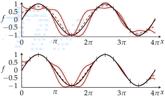
Figure 2. Top: real function $f=sin$ () and GPR with mean m () and covariance function C where () symbolizes mean plus/minus standard deviation (i.e., $m\left(x\right)\pm \sqrt{C(x,x)}$) at each point. Bottom: Same as top with m and C conditioned to the vertical cyan dashes.

3.2. GPR Hyperparameter Adaption

Using a GPR for supervised learning problems requires the choice of some (initial) mean function and covariance function (Theorem 3). Most examples of covariance functions involve the choice of hyperparameters. Example 4 involves the choice of a lengthscale and output variance.

Consider a supervised learning problem $f:X\to ℝ$ with training points $T=\{(x_1,y_1),\dots ,(x_N,y_N)\}\subset X\times ℝ$. Given a mean function m and a family of covariance functions $C_{\theta }$ with $\theta$ element of some index set $\vartheta$, we choose a hyperparameter $\theta$ by following the maximum likelihood principle.

Denote by $f_{C,m,\theta }$ the density function of the multivariate normal distribution

$$\mathcal{N}(m_{\{x_1,\dots ,x_N\}},C_{\theta ,\{x_1,\dots ,x_N\}}).$$

We choose $\theta$ by solving

$${\theta }^{*}=\underset{\theta \in \vartheta }{argmax}(f_{C,m,\theta }({\left(y_i\right)}_{i=1,\dots ,N})).$$

(4)

Remark 3.

In practice, one often replaces $f_{C,m,\theta }$ with $ln{f}_{C,m,\theta }$ and solves

$${\theta }^{*}=\underset{\theta \in \vartheta }{argmax}(ln{f}_{C,m,\theta }({\left(y_i\right)}_{i=1,\dots ,N}))$$

(5)

resulting in identical parameters. However,

$$\begin{array}{c}\hfill ln{f}_{C,m,\theta }\left(y\right)=-\frac{1}{2}{y}^{\top }{C}_{\theta ,\{x_1,\dots ,x_N\}}y-\frac{1}{2}ln(det\left(C_{\theta ,\{x_1,\dots ,x_N\}}\right)-\frac{N}{2}ln\left(2\pi \right)\end{array}$$

is more convenient to work with.

3.3. Bayesian Optimization

We define the hypervolume improvement as the gain of hypervolume when adding new points. At some places, the underlying function used for calculating new sample (or infill) points is called acquisition function.

Definition 5 (Hypervolume Improvement).

Given a reference point $r\in {ℝ}^t$ and a finite set of vectors $F\subset {ℝ}^t$, the hypervolume improvement of some $y\in {ℝ}^t$ is defined as

$$\begin{array}{c}\hfill {HVI}_r(F,y)={HV}_r(F\cup \left\{y\right\})-{HV}_r\left(F\right).\end{array}$$

(6)

We denote by

$$\begin{array}{c}\hfill {HVI}_{r,F}:{ℝ}^t\to ℝ,y\mapsto {HVI}_r(F,y)\end{array}$$

(7)

the resulting function. We often write ${HVI}_r$ instead of ${HVI}_{r,F}$ whenever F is clear from context. Observe that ${HVI}_{r,F}$ is continuous (see Appendix C), hence integrable, on a bounded subset.

Remark 4.

Maximizing the Hypervolume improvement results in Pareto points (see Proposition 1).

Consider a black box function $f:X\to {ℝ}^t$ with evaluations $T=\{(x_1,y_1),\dots ,(x_N,y_N)\}\subset X\times {ℝ}^t$. Given an approximation $\widehat{f}$ of f (such as the mean of a GPR) and a suitable reference point $r\in {ℝ}^t$, we strive to calculate

$$\underset{x\in X}{\mathrm{argmax}}{HVI}_r(\{y_1,\dots ,y_N\},\widehat{f}\left(x\right))$$

in order to find a preimage of a Pareto point of f.

Recall that GPRs include a prediction uncertainty measure (Remark 2). We can take this additional information into account when maximizing the Hypervolume improvement in the following ways.

Definition 6 (Expected Hypervolume Improvement).

Let mean functions $m_i:X\to ℝ$ and covariance functions $C_i:X\times X\to ℝ$ on X for $i=1,\dots ,t$ be given. Denote by

$$m\left(x\right)={\left(m_i\left(x\right)\right)}_{i=1,\dots ,t}$$

the induced mean vector and by $C\left(x\right)$ the diagonal matrix with

$$C{\left(x\right)}_{ii}=C_i(x,x).$$

Then, the expected Hypervolume improvement at $x\in X$ is given by the expected value

$$EHVI\left(x\right)={\int }_{y\in {ℝ}^t}{HVI}_r\left(y\right)d{P}_x={\int }_{y\in {ℝ}^t}{HVI}_r\left(y\right)f_{m\left(x\right),C\left(x\right)}dy$$

(8)

of HVI with respect to the probability measure

$$P_x={\otimes }_{i=1}^t\mathcal{N}(m_i\left(x\right),C_i(x,x))=\mathcal{N}(m\left(x\right),C\left(x\right))$$

on ${ℝ}^t$.

In many situations, the training data (more precisely the evaluations) are manipulated (i.e., pre-processed) before training (i.e., calculating the hyperparamters of the means und covariance functions). By the very definition, we obtain the following corollary:

Corollary 7.

Let $S\subset {ℝ}^t$ and $g:S\to {ℝ}^t$ be a function. Assume g satisfies $a_i<b_i$ if and only if $g{\left(a\right)}_i<g{\left(b\right)}_i$ for all $i=1,\dots ,t$ and $a,b\in S$. Then, $s\in S$ is a Pareto point if and only if $g\left(s\right)\in g\left(S\right)$ is a Pareto point.

Therefore, any function satisfying the above assumptions may be used for pre-processing of data points in the context of multicriterial optimization.

Remark 5.

The expected Hypervolume improvement involves the choice of some reference point. By construction, this choice affects the (expected) hypervolume contribution of any point in the target space. Notice that the reference point must be strictly greater in every component than every pareto optimal solution in order to ensure a hypervolume greater than zero for every such point. For example, if the black box function f factorizes through ${[0,1]}^t\subset {ℝ}^t$, then, such a reference point may be chosen by

$$(1+\epsilon ,\dots ,1+\epsilon )\in {ℝ}^t$$

(9)

for some $\epsilon >0$.

Further discussion for the reference point selection may be found in the literature, e.g., under [17].

Roughly speaking, the expected hypervolume improvement is an extension of the hypervolume improvement incorporating the uncertainty information encapsulated in the GPRs. One hopes that maximizing the expected hypervolume improvement (of the GPRs) maximizes the hypervolume improvement of the black box function more efficiently than simply maximizing the hypervolume of the underlying mean function of the GPRs. Note that incorporating the uncertainty (of the model) allows to reflect a trade-off between exploration and exploitation.

3.4. Summary—Base for an Algorithmic Implementation

We shortly summarize the necessary steps in order to apply GPR and EHVI based multicriterial optimization to a black box function

$$f:X\to {ℝ}^t.$$

Let

$$T=\{(x_1,y_1),\dots ,(x_N,y_N)\}\subset X\times {ℝ}^t$$

be evaluations of f. We define $X_0=\{x_1,\dots ,x_N\}$ and $Y_0=\{y_1,\dots ,y_N\}$.

3.4.1. Setting up the GPRs

For each $i=1,\dots ,t$ we choose a mean function $m_i$ and a covariance function (i.e., a positive quadratic form) $C_i$ on X. Examples of covariance functions can be found in [16]. By Theorem 3, we obtain a Gaussian Process for each i. In case the covariance function involves the choice of some hyperparameter, we determine that parameter by solving Equation (5). Next, we condition each mean $m_i$ and covariance function $C_i$ to T using Equations (2) and (3), respectively. We obtain GPRs, defined by their conditioned mean $m_i^{\prime }$ and covariance function $C_i^{\prime }$ for each $i=1,\dots ,t$ (i.e., for each output component).

3.4.2. Maximizing the EHVI

We maximize the expected Hypervolume improvement, i.e., we solve

$$p=\underset{x\in X}{argmax}EHVI\left(x\right)$$

(10)

according to Equation (8) with respect to the mean functions $m_i^{\prime }$ and covariance functions $C_i^{\prime }$. Algorithms for calculation of the expected Hypervolume improvement may be found in [18,19]. Lastly, we evaluate the black box function f at the found p.

We close this section by a couple of practical remarks:

• GPRs form a rich class of regression models. However, evaluating a GPR involves the inversion of a $N\times N$ matrix with N being the number of training points (see Equation (3)). Accordingly, evaluating a GPR tends to get slow with increasing number of training points.
• In addition, GPRs (as any regression model) requires a careful pre-processing of the data in order to produce reasonable results. At the very least, the input and output of the training data should be normalized (e.g, to $(0,1)$).

To enable the reader understanding the GPR-MOBO algorithm described below in a comprehensible way, we present here a pre-processing example of the training data: Denote by

$$x_{min}={(\underset{z\in X}{inf}\left(z_i\right))}_{i=1,\dots ,d}\mathrm{and}{x}_{max}={(\underset{z\in X}{sup}\left(x_i\right))}_{i=1,\dots ,d}$$

the componentwise minimum resp. maximum within the design space X. Then, define

$$n_X:X\to {[0,1]}^d,x\mapsto \frac{x-x_{min}}{x_{max}-x_{min}}$$

(11)

where the division is performed componentwise and $X_n=n_X\left(X_0\right)$. Assuming X to be bounded and $x_{max,i}\ne x_{min,i}$ for all components i, this is well defined. Furthermore, we define

$$y_{min}={(\underset{y\in Y_0}{min}\left(y_i\right))}_{i=1,\dots ,t}\mathrm{and}{y}_{max}={(\underset{y\in Y_0}{max}\left(y_i\right))}_{i=1,\dots ,t}$$

by componentwise minimum resp. maximum of the evaluations. Without loss of generality, we may assume $y_{max,i}\ne y_{min,i}$ for all i. Define

$$n_Y:{ℝ}^t\to {ℝ}^t,y\mapsto \frac{y-y_{min}}{y_{max}-y_{min}}$$

(12)

and $Y_n=n_Y\left(Y_0\right)$. It is straightforward to check that $n_Y$ satisfies the assumptions of Corollary 7.

We obtain normalized training data

$$\begin{array}{c}\hfill T_n=\{(n_X\left(x_1\right),n_Y\left(y_1\right)),\dots ,(n_X\left(x_N\right),n_Y\left(y_N\right))\}\subset {[0,1]}^d\times {[0,1]}^t.\end{array}$$

4. Algorithmic Implementation and Validation

In this section, we first derive an algorithmic implementation of an adaptive Bayesian Optimization (BO) algorithm based on GPR infill making use of expected hypervolume improvement as acquistion function. in Section 4.2, we apply this algorithm to a mathematical test function with known Pareto front prior validating it in Section 4.3 within context of a real-world power system application.

4.1. GPR-MOBO Algorithmic Implementation

The proposed GPR-MOBO workflow presented in Algorithm 1 strictly follows the sequence of steps for applying GPR with EHVI-based MOO to a black box function as described in Section 3.4.

Algorithm 1 Structural MO Bayesian Optimization workflow.
$X_0\leftarrow \{x_1,\dots ,x_{N_0}\}$	▷ Set initial DoE
$Y_0\leftarrow f\left(X_0\right)$	▷ Simulate at $X_0$ (expensive)
$m\leftarrow 0_{\mathrm{map}}$	▷ Choose zero map as mean function
$C\leftarrow$(1)	▷ Choose covariance function
$r\leftarrow$(9)	▷ Choose reference point
while $|X_0|<N_{\mathrm{tot}}$ do	▷ unless abortion criterion is met
$X_{\mathrm{n}},Y_{\mathrm{n}}\leftarrow$(11), (12)	▷ Pre-process data
for $i=1\dots t$ do	▷ for each dimension of target space
${\theta }_i^{*}\leftarrow$(5)	▷ Calculate hyperparameters
$m_i^{\prime }\leftarrow$(2)	▷ Condition mean
$C_i^{\prime }\leftarrow$(3)	▷ Condition covariance
end for
$p\leftarrow$(10)	▷ Calculate optimal infill sample point
$X_0\leftarrow X_0\cup \left\{n_X^{-1}\left(p\right)\right\}$	▷ Add infill to $X_0$
$Y_0\leftarrow Y_0\cup \left\{f\left(n_X^{-1}\left(p\right)\right)\right\}$	▷ Add simulation at $n_X^{-1}\left(p\right)$ to $Y_0$ (expensive)
end while
$Y_P\leftarrow \{y_1,\dots ,y_k\}$	▷ Find non-dominated points
$X_P\leftarrow f^{-1}\left(Y_P\right)$	▷ Acquire according design space points
return $X_P,Y_P$

Wherever applicable, we refer to equations as referenced in Section 3. As an initial design of experiments (DoE) $X_0$, we propose Latin Hypercube Sampling (LHCS) according [20] as the basis of the initial computationally expensive black box function evaluation $f\left(X_0\right)$. We assume the initial sampling by $N_0$ expensive evaluations to cover the full range of parameter values within the target space to guarantee its image on unit cube after normalization.

$N_{\mathrm{tot}}$ (maximum number of samples available for computationally expensive black box function evaluations) and $N_0$ (fraction of $N_{\mathrm{tot}}$ as the number of initial samples) may be considered as the GPR-MOBO hyperparameters.

Algorithm 1 has been implemented in Matlab 2021b making use of the minimizer fmincon based on the sqp option (called multiple times with different initial values by GlobalSearch) to find the minimum of the negative log marginal likelihood function for hyperparameter adaption (see Section 3.2) and for BO (see Section 3.3) with application to the negative EHVI function which is provided by [21]. At this point it seems worthwhile noting, GlobalSearch not to yield deterministic results, i.e., multiple runs with identical input values may vary in their output values.

To make the computation more efficient, for numerical inversion of $C_F$, the Cholesky decomposition is used.

4.2. Test Function Based Validation

In this subsection, we are aiming for an effectiveness and efficiency comparison of Algorithm 1 versus state-of-the-art alternatives LHCS [20] and NSGA-II [22]. We present results of their application to a well defined black box function with analytically well known Pareto front. In our case, we picked the to be minimized test function ZDT1 according [22]

$$\begin{array}{c}\hfill f:{[0,1]}^d\to {ℝ}^2,\left(\begin{array}{c}{x}_1\\ ⋮\\ x_d\end{array}\right)\mapsto \left(\begin{array}{c}{x}_1\\ g\left(x\right)\left[1-\sqrt{\frac{x_1}{g\left(x\right)}}\right]\end{array}\right)\mathrm{with}g\left(x\right)=1+\frac{9}{d-1}\sum _{i=2}^d{x}_i\end{array}$$

and $2\le d\le 30$ indicating the design space dimension. Note that ZDT1 exhibits a convex Pareto front independent of d.

We compare results for the alternative Pareto front search algorithms granting $N_{\mathrm{tot}}=50$ black box evaluations plus adding an NSGA-II analysis with $N_{\mathrm{tot}}=200$ black box evaluations. For LHCS, all samples were spent within the initial run while Algorithm 1 started with $N_0=30$ initial LHCS samples. In case of $N_{\mathrm{tot}}=50$ total samples, the NSGA-II algorithm was applied in $n_{\mathrm{gen}}=5$ generations with a population of $n_{\mathrm{pop}}=10$ samples while in case of $N_{\mathrm{tot}}=200$ total samples, $n_{\mathrm{gen}}=8$ generations with a population of $n_{\mathrm{pop}}=25$ samples were run. For statistical purposes, the algorithm evaluations were repeated fifty times with different random starting values. Design space dimension was chosen by $d\in \{2,3,5,10,15,20,25,30\}$. The reference point during optimization was chosen according Equation (9) with $\epsilon =2\%$. Making use of knowledge about the ZDT1 target domain, we fixed $y_{min}=(0,0)$ for pre-processing. To quantify the search algorithms’ performance, the hypervolume with respect to reference point $(2,10)$ in relation to the (known) maximal hypervolume is evaluated. The results are plotted in Figure 3.

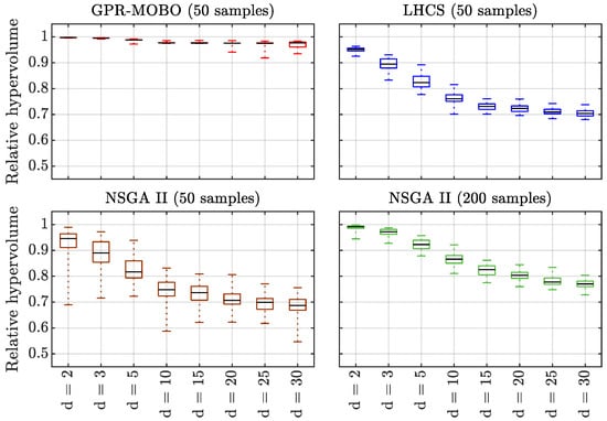
Figure 3. Statistical evaluation of relative hyper volume from 50 repeated runs comparing performance of three MOO algorithms for a selected set of ZDT1 design space dimension d. Top three evaluations for GPR-MOBO ($N_0=30$ initial samples, red), LHCS (blue) and NSGA-II (with $n_{\mathrm{pop}}=10$ samples in $n_{\mathrm{gen}}=5$ generations, brown) are based on $N_{\mathrm{tot}}=50$ samples. Bottom figure evaluation for NSGA-II ($n_{\mathrm{pop}}=25$ samples in $n_{\mathrm{gen}}=8$ generations, (green) is based on $N_{\mathrm{tot}}=200$ samples.

Box plots in Figure 3 indicate statistical evaluations of the repeated search runs. GPR-MOBO results are drawn in red, LHCS results in blue, NSGA-II results for $N_{\mathrm{tot}}=50$ in brown and for $N_{\mathrm{tot}}=200$ in green.

4.3. Power System Design Based Validation

Within the last subsection of this chapter, we apply the GPR-MOBO Algorithm 1 to the design and optimization of a power system example. Figure 4 illustrates both, the toolchain and the generic power system model as used for GPR-MOBO power system design and optimization validation.

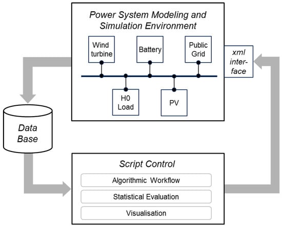
Figure 4. Toolchain and generic power system model as used for GPR-MOBO power system design based validation.

For the energy domain specific “Power System Modeling and Simulation Environment” of the tool chain in our example, we use the commercial tool PSS^®DE [23]. Connected to the “Script Control” (implemented in Python code) through an “xml interface”, adjustable design space parameters of the power system model receive dedicated parameter values as computed within the “Algorithmic Workflow” (execution of the GPR-MOBO algorithm in Matlab 2021b code). Data stored within the “Data Base” are accessible for “Statistical Evaluation” and “Visualisation” (all implemented in Python code). The generic power system model for our validation example is defined by a star topology connecting a standard $H0$-profile [24] electric load with $20.2$ GWh annual demand to three aggregate components (“Wind turbine”, “PV”, “Battery”) and a “Public Grid”. The “Power System Modeling and Simulation Environment” is simulating power system results in terms of well defined key performance indicators (KPI), CAPEX (captial expenditures for installation of the according power system), and CO₂ (amount of carbon dioxide for a given configuration to provide the total amount of energy). The KPI behavior of the “Power System Modeling and Simulation Environment” can therefore be viewed as a black box function.

Parameter value ranges defining the design space for the system of interest are listed in Table 1.

Table 1. Design space limits for the experiment.

Design Parameter	Min	Max
PV peak power/MW${}_{\mathrm{p}}$	0	41
Wind turbine peak power/MW${}_{\mathrm{p}}$	0	$17.1$
Battery rack capacity/MAh	0	$1.21$

As mentioned in Section 3.3, for the GPR-MOBO, the design and target space samples (design parameters and KPIs, respectively) are normalized according Equations (11) and (12).

The results for the experiment are shown in Figure 5. $N_0=30$ initial samples and $N_{\mathrm{tot}}=50$ samples in total were chosen as GPR-MOBO hyperparameters, while total emission of carbon dioxide (CO₂ in kilotons) and capital expenditures for acquisition and installation of aggregate components (CAPEX in million euros) were selected as to be evaluated trade-off KPIs. Making use of knowledge about the according target domain, we fixed $y_{min}=(0,0)$ for pre-processing. The reference point during optimization was chosen according Equation (9) with $\epsilon =2\%$.

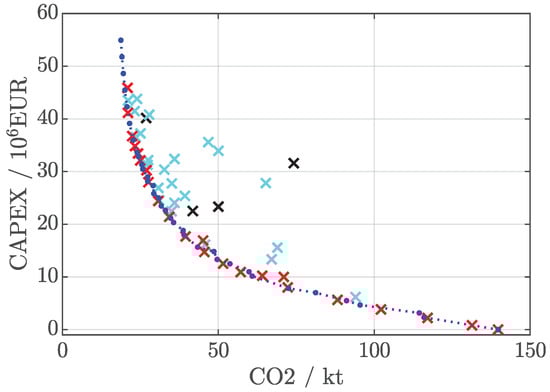
Figure 5. CAPEX vs. CO₂ evaluations (marked by crosses) as obtained by power system simulation. Initial samples are marked by ×, Pareto-optimal samples by ×. An approximate Pareto front based on 1200 full-factorial design space latticing sample points is indicated by blue dots with interpolation marked by a blue dotted line .

Figure 5 shows the acquired subspace of the target space by the experiment. All sample points are marked by crosses, while the Pareto optimal solutions forming the Pareto front are highlighted by red crosses × and the remaining portion of initial (30 LHCS) results are marked by cyan crosses ×. In addition, an approximate Pareto front is plotted, resulting from a full-factorial design space latticing based on 1200 sample points. Non-dominated Pareto points are indicated by blue dots with a Pareto front completed by linear interpolation (marked by a blue dotted line ).

5. Discussion

According Section 2, we may interpret the identified hypervolume of a black box as an indicator of effectiveness for a given Pareto front search algorithm. Putting that identified hypervolume in ratio to the number of computationally expensive evaluations required to identify this hypervolume, in turn, may be considered a suitable indicator of the algorithm’s efficiency. Applying these definitions to results obtained in the previous Section 4, Figure 3 clearly indicates:

(i)

Given the limited low number of $N_{\mathrm{tot}}=50$ samples, all selected algorithms indicate a decreasing effectiveness over an increasing number of design space dimensions (i.e., degrees of design freedom, DoF).

(ii)

GPR-MOBO outperforms the effectiveness of the other algorithms for all DoF d, showing even for $d=30$ (with $N_{\mathrm{tot}}=50)$ at the median more than $97\%$ effectiveness (versus less than $71\%$ for the other algorithms).

(iii)

For $N_{\mathrm{tot}}=50$, the effectiveness of NSGA-II and LHCS appears comparable within statistical significance for all evaluated DoF n.

(iv)

For $N_{\mathrm{tot}}=50$ samples, GPR-MOBO outperforms NSGA-II even when applied with $N_{\mathrm{tot}}=200$ samples.

(v)

Efficiency of GPR-MOBO significantly increases with increasing DoF n when compared to other algorithms.

On the other hand, it is worthwhile mentioning GPR-MOBO algorithm to require more computation time than standard LHCS or NSGA-II algorithms. Depending on the test function dimension d and hardware environment, GPR-MOBO runs (i.e., 20 iterations) took between $3 \min$ and $11 \min$ wherein the fraction for evaluating the black box function (ZDT1) can be treated as negligible while NSGA-II or LHCS runs tool only less than a tenth portion of this time. This indicates that the GPR-MOBO is advisable, if the black box function is expensive to evaluate in terms of capital, time, or other resources.

The experimental validation using an unknown black box function whose result is shown in Figure 5 again validates the effectiveness and efficiency of the GPR-MOBO. The Pareto front as identified by $N_{\mathrm{tot}}=50$ black box evaluations is already very close to the front as approximated by $N_{\mathrm{tot}}=1200$ full-factorial lattice based black box evaluations. Some GPR-MOBO Pareto points are even dominating that identified by full-factorial lattice. The example, thereby, demonstrates effectiveness and efficiency of GPR-MOBO based power system design and optimization.

The results shown indicate a general superiority of GPR-MOBO over state-of-the-art algorithms. However, this has been demonstrated only on exemplary base. We therefore point out the inadmissibility of a generalization of superiority. A general superiority of GPR-MOBO cannot and should not be derived from single, individual test functions or application examples. Such a fundamental superiority would have to be mathematically proven and would presumably require fundamental knowledge of the black box function itself or the Pareto front spanned by this black box function.

6. Conclusions and Outlook

In this paper, we tackled the challenge of power system design and optimization in VUCA environment. We proposed a Multi-Objective Bayesian Optimization based on Gaussian Process Regression (GPR-MOBO) in the context of power system virtual prototyping. After a mathematical reformulation of the challenge, we presented the background of Gaussian Process Regression, including hyperparameter adaption and use in the context of a Bayesian Optimization approach, focusing on the expected improvement in hypervolume. For validation purposes, we benchmarked our GPR-MOBO implementation statistically based on a mathematical test function analytically known Pareto front and compared results to those of well-known algorithms NSGA-II and pure Latin Hyper Cube Sampling. We demonstrated superiority of the GPR-MOBO approach over the compared algorithms, especially for high dimensional design spaces. Finally, we applied the GPR-MOBO algorithm for planning and optimization of a power system (energy park) in terms of selected performance indicators of exemplary character.

Concluding, GPR-MOBO turned out as an effective and efficient approach for power system design and optimization in VUCA environment with superior character when simulations are computationally expensive and the number of design degrees of freedom is high.

Some topics remain open for future investigation. Besides a performance comparison with other than already selected algorithms, some detailed questions within the GPR-MOBO family are worthwhile to be considered. This includes topics such as the choice of acquisition function, pre-processing, selection of the reference points when (expected) hypervolume (improvement) is put in focus and application of various global optimizers to name just a few. One level above, more not yet satisfactorily answered question address the extension to mixed-integer design spaces and issues related to constraint handling.

References

- Elkington, R. Leadership Decision-Making Leveraging Big Data in Vuca Contexts. J. Leadersh. Stud. 2018, 12, 66–70. [Google Scholar] [CrossRef]
- Afshari, H.; Hare, W.; Tesfamariam, S. Constrained multi-objective optimization algorithms: Review and comparison with application in reinforced concrete structures. Appl. Soft Comput. 2019, 83, 105631. [Google Scholar] [CrossRef]
- Shahriari, B.; Swersky, K.; Wang, Z.; Adams, R.P.; de Freitas, N. Taking the Human Out of the Loop: A Review of Bayesian Optimization. Proc. IEEE 2016, 104, 148–175. [Google Scholar] [CrossRef]
- Lyu, W.; Xue, P.; Yang, F.; Yan, C.; Hong, Z.; Zeng, X.; Zhou, D. An Efficient Bayesian Optimization Approach for Automated Optimization of Analog Circuits. IEEE Trans. Circuits Syst. I Regul. Pap. 2018, 65, 1954–1967. [Google Scholar] [CrossRef]
- Zhang, S.; Yang, F.; Yan, C.; Zhou, D.; Zeng, X. An Efficient Batch-Constrained Bayesian Optimization Approach for Analog Circuit Synthesis via Multiobjective Acquisition Ensemble. IEEE Trans.-Comput.-Aided Des. Integr. Circuits Syst. 2022, 41, 1–14. [Google Scholar] [CrossRef]
- Guo, J.; Crupi, G.; Cai, J. A Novel Design Methodology for a Multioctave GaN-HEMT Power Amplifier Using Clustering Guided Bayesian Optimization. IEEE Access 2022, 10, 52771–52781. [Google Scholar] [CrossRef]
- Sawant, M.M.; Bhurchandi, K. Hierarchical Facial Age Estimation Using Gaussian Process Regression. IEEE Access 2019, 7, 9142–9152. [Google Scholar] [CrossRef]
- Huang, H.; Song, Y.; Peng, X.; Ding, S.X.; Zhong, W.; Du, W. A Sparse Nonstationary Trigonometric Gaussian Process Regression and Its Application on Nitrogen Oxide Prediction of the Diesel Engine. IEEE Trans. Ind. Inform. 2021, 17, 8367–8377. [Google Scholar] [CrossRef]
- Koriyama, T.; Nose, T.; Kobayashi, T. Statistical Parametric Speech Synthesis Based on Gaussian Process Regression. IEEE J. Sel. Top. Signal Process. 2014, 8, 173–183. [Google Scholar] [CrossRef]
- Schulz, E.; Speekenbrink, M.; Krause, A. A tutorial on Gaussian process regression: Modelling, exploring, and exploiting functions. J. Math. Psychol. 2018, 85, 1–16. [Google Scholar] [CrossRef]
- Lewis-Beck, C.; Lewis-Beck, M. Applied Regression: An Introduction; Sage Publications: Thousand Oaks, CA, USA, 2015; Volume 22. [Google Scholar]
- Verleysen, M.; François, D. The curse of dimensionality in data mining and time series prediction. In Proceedings of the International Work-Conference on Artificial Neural Networks, Barcelona, Spain, 8–10 June 2005; Springer: Berlin/Heidelberg, Germany, 2005; pp. 758–770. [Google Scholar]
- Frazier, P.I. Bayesian optimization. In Recent Advances in Optimization and Modeling of Contemporary Problems; Informs: Phoenix, AZ, USA, 2018; pp. 255–278. [Google Scholar]
- Emmerich, M.; Deutz, A.H. A tutorial on multiobjective optimization: Fundamentals and evolutionary methods. Nat. Comput. 2018, 17, 585–609. [Google Scholar] [CrossRef] [PubMed]
- Anderson, T.W. An Introduction to Multivariate Statistical Analysis, 3rd ed.; Wiley: New York, NY, USA, 2003. [Google Scholar]
- Duvenaud, D. Automatic Model Construction with Gaussian Processes. Ph.D. Thesis, University of Cambridge, Cambridge, UK, 2014. [Google Scholar]
- Ishibuchi, H.; Imada, R.; Setoguchi, Y.; Nojima, Y. Reference point specification in hypervolume calculation for fair comparison and efficient search. In Proceedings of the Genetic and Evolutionary Computation Conference, Berlin, Germany, 15–19 July 2017; pp. 585–592. [Google Scholar]
- Emmerich, M.; Deutz, A.; Klinkenberg, J. Hypervolume-based expected improvement: Monotonicity properties and exact computation. In Proceedings of the 2011 IEEE Congress of Evolutionary Computation (CEC), Ritz Carlton, New Orleans, LA, USA, 5–8 June 2011; pp. 2147–2154. [Google Scholar]
- Yang, K.; Emmerich, M.; Deutz, A.; Bäck, T. Efficient computation of expected hypervolume improvement using box decomposition algorithms. J. Glob. Optim. 2019, 75, 3–34. [Google Scholar] [CrossRef]
- McKay, M.D.; Beckman, R.J.; Conover, W.J. A Comparison of Three Methods for Selecting Values of Input Variables in the Analysis of Output from a Computer Code. Technometrics 1979, 21, 239. [Google Scholar]
- Emmerich, M. KMAC V1.0 - The efficient O(n log n) implementation of 2D and 3D Expected Hypervolume Improvement (EHVI). Available online: https://liacs.leidenuniv.nl/~csmoda/index.php?page=code (accessed on 22 June 2022).
- Deb, K.; Pratap, A.; Agarwal, S.; Meyarivan, T. A fast and elitist multiobjective genetic algorithm: NSGA-II. IEEE Trans. Evol. Comput. 2002, 6, 182–197. [Google Scholar] [CrossRef]
- Siemens, Data Sheet PSS®DE. Available online: https://new.siemens.com/global/en/products/energy/energy-automation-and-smart-grid/grid-edge-software/pssde.html (accessed on 24 August 2022).
- Proedrou, E. A comprehensive review of residential electricity load profile models. IEEE Access 2021, 9, 12114–12133. [Google Scholar] [CrossRef]
- Georgii, H.O. Stochastik: Einführung in die Wahrscheinlichkeitstheorie und Statistik, 5. Auflage; Walter de Gruyter: Berlin, Germany, 2007. [Google Scholar]
Publisher’s Note: MDPI stays neutral with regard to jurisdictional claims in published maps and institutional affiliations. |
© 2022 by the authors. Licensee MDPI, Basel, Switzerland. This article is an open access article distributed under the terms and conditions of the Creative Commons Attribution (CC BY) license (https://creativecommons.org/licenses/by/4.0/).