Article

Fiscal Policy Effects on Private Expenditure for Sustainable Economic Growth: A Panel VAR Study from Selected Developing Countries

by
Iszan Hana Kaharudin
1,* and
Mohammad Syuhaimi Ab-Rahman
2
1
Centre for Liberal Studies (CITRA), Universiti Kebangsaan Malaysia, Bangi 43600, Malaysia
2
Center of Alumni Engagement, Universiti Kebangsaan Malaysia, Bangi 43600, Malaysia
*
Author to whom correspondence should be addressed.
Sustainability 2022, 14(17), 10786; https://doi.org/10.3390/su141710786
Submission received: 12 June 2022 / Revised: 17 August 2022 / Accepted: 18 August 2022 / Published: 30 August 2022

Abstract

:
This study examines the effects of fiscal policy on private expenditure using a panel VAR for the sample of 60 developing countries from 1990 to 2020. The VAR panel model framework was used to focus on the disaggregated government expenditures which included the defense, economic and social expenditure. The main findings showed a positive shock effect of defense expenditure which led to crowding out effect on private expenditure and domestic income. Conversely, economic and social expenditure had the crowding in effect on private consumption and domestic income. To detail out the analysis, the composition of government spending was divided into two, namely productive expenditures and non-productive expenditures. Therefore, the findings indicate that defense expenditure is non-productive since it does not stimulate an increase in private spending and national income while economic expenditure and social expenditure are classified as productive expenditure with the ability to increase economic activity. The policy implication suggests that the government should carefully examine and identify the sectors or composition that have greater potential, capacity and relevance in stimulating sustainable economic growth.

1. Introduction

Theoretical differences on the impact of the expansion of fiscal policy on economic activity have led to some empirical studies to support the respective theories. Unfortunately, the results were rather mixed without clear support for any particular theory. The situation therefore requires a more detailed study in order to conclusively identify the most appropriate theory to relate the impact of fiscal policy to economic activity.
Fiscal policy is the tool to influence the economic growth through increasing government spending and reducing taxation. Governments typically use fiscal policy to promote strong and sustainable economic growth and reduce poverty. However, increasing government spending may lead to a crowding out effect on private investment. In economics, crowding out refers to the effects on expanding the economy because of the implementation of fiscal policy by the government. The increase in government expenditures leads to a negative effect on private expenditure. If an increase in government expenditure fails to increase economic growth, then private sector expenditure such as private investment and private consumption is said to promote a crowding out effect and thus retard sustainable economic growth.
Many economists were interested in studying the relationship between government expenditure and private investment, especially in terms of the impact of the former. However, the results of empirical research in this area were controversial. Aschauer [1] and Monadjemi [2] stated that there was substitutability between government expenditure and private investment, whereas Aschauer [3], Erenburg et al. [4], Bairam et al. [5], Karras [6], Erenburg et al. [7] and Argimon et al. [8] instead supported their complementarity. Similarly, recent studies by Sie et al. [9] found that private investment crowding in education and defense of government expenditures was significant in the long term. Hussain et al. [10] also found that development expenditure such as those on infrastructure, health and education, crowded in or stimulated private investment.
This paper aims to measure the contribution of each sector, either productive or unproductive, to sustainably boost economic growth in the developing countries (NSM). Therefore, the main objective of this study is to examine the effects of disaggregated government expenditure on private expenditure which includes the categories of government expenditure such as defense expenditure, economic expenditure and social expenditure.
This study significantly contributes to the literature, through the improvement and extension of existing research. In lieu of improvement, the study has disaggregated government expenditure to defense, economic and social expenditures. Most of the extant empirical works that exist have examined the aggregate government expenditure rather than disaggregated government spending such as studies by Heppke-Falk et al. [11], Gali et al. [12], Afonso et al. [13,14] and Yadav et al. [15]. Aggregation in these studies were unclear and less detailed as compared to those relating to disaggregated government expenditure.
The remainder of the paper is organized as follows: Section 2 presents the literature review, Section 3 focuses on the research methodology, Section 4 discusses the empirical results of the study and Section 5 summarizes and concludes the study.

2. Literature Review

The literature mainly focuses on aggregated rather than disaggregated government expenditure such as defense, economic and social expenditure on economic growth and private expenditure. Thus, the novelty of this research is to explore the disaggregated government expenditure on private expenditure and economic growth. Aschauer [3] stated that the relationships between government expenditure and private investment are important to distinguished between different categories of expenditure such as those on roads, education and airports, and research may increase the productivity of the private sector and also complement private investment expenditure. Results showed that there is an expansion rather than contraction in private investment. However, the government expenditure in areas such as food, health and defense may substitute for private consumption expenditure.
Monadjemi [2] examined the effect of government spending on private investment in the United Kingdom and the United States using quarterly data spanning 1960–1991. The study employed variance decomposition derived from the error correction model. The results indicated that defense and social welfare expenditures are the most important variables influencing private investment in the United States, whereas government expenditure is the relatively more important variable in the United Kingdom and the results from Wang et al. [16] show that defense expenditure is important for improving economic productivity in OECD countries using Malmquist productivity Index (MPI). The authors indicated that higher economic productivity is associated with defense expenditure. Studies in European countries, namely Greece, Ireland, Portugal and Spain carried out by Laopodis [17] have examined the effect of military and non-military public expenditure on gross private investment using co-integration analysis and error correction analysis. The period of study was from 1960 to 1997. The latter type of public expenditure was disaggregated into defense, public capital, consumption and others. The results suggest that public capital expenditure reduces private investment in Spain. Three other countries show public capital expenditure stimulating private investment. Additionally, defense spending has not affected private investment, thus extending the ongoing controversy related to the economic effects of military spending.
The method of financing government expenditure as either tax-financed or debt-financed has played an important role in determining the effect of government spending on economic growth. Miller et al. [18] studied the effect of fiscal policy on economic growth using samples from developed and developing countries spanning 1975–1984. Results showed that for developing countries, debt-financed increases in government expenditure retarded economic growth whereas tax-financed increases led to stimulated economic growth. For developed countries, debt-financed increases in government expenditure do not affect economic growth and tax-financed increases led to lower growth. Secondly, different government expenditures affect economic growth differently. Debt-financed increases in defense, health and social security and welfare expenditure showed negative impact on economic growth in developing countries. Conversely, debt-financed increases in education and expenditure stimulated economic growth in developed countries. In addition, Mahmoudzadeh et al. [19] evaluated the effect of disaggregated fiscal spending (consumption, capital formation and budget deficit) on private investment in both developed and developing countries using a panel data, spanning 2000 to 2009. The results indicated that the elasticity of private investment with respect to government capital formation expenditure is positive for both groups, but the complementary effect is greater than in the developed countries. Likewise, the elasticity of private investment with respect to government consumption expenditure is significantly negative in both groups, but the substitution effect is larger in developed countries. Furthermore, the effect of a budget deficit crowd out private investment in developed countries, while it has a positive effect in developing countries. However, these effects are marginal in both groups.
Ahmed and Miller [20] studied the effect of disaggregated government expenditure on private investment using fixed-effect and random-effect methods. The study used panel data methods to test 39 countries (23 developing countries and 16 countries) based on Summers and Heston data. Using the government budget constraint, they explored the effects of tax-financed and debt-financed expenditure for the full sample and sub samples of both developed and developing countries. They ran two sets of regressions with one set on total government expenditure and the other on disaggregated expenditure item. Each of the government expenditures was divided into several subsectors such as defense, education, health, social security and welfare, service and economic relations, transportation and communication. The findings showed that tax-financed government expenditure crowded out more investment than debt-financed spending. Expenditure on social security and welfare reduced private investment while transport and communications induced private investment in all samples. Tax-financed government expenditure showed that all government spending crowded out private investment except transportation and communication expenditure, which crowded in private investment for all countries. However, for developing countries only, transportation and communications still induced private investment while social security and welfare still reduce private investment. In developed countries, expenditure on health, social security and welfare reduced private investment.
Wang [21] has disaggregated government expenditure into five categories of expenditure. The author examined the relationship between government expenditures and private investment in Canada during the period 1961 to 2004 using Johansen and Juselius integration analysis and error variable model (ECM). Results indicated that government expenditure on education and health has a positive effect on private investment whereas government expenditures on capital and infrastructure similarly showed positive effects. The other expenditures, including those on protection of persons and property, social service and debt charges have no significant effects on private investment. Hussain et al. [10] divided government expenditure into two categories: namely, current expenditure and development expenditure. The authors examined the long-term relationship between government spending and private investment in Pakistan using time series annual data, spanning 1975 to 1980. Results indicated that current expenditures, such as defense and debts served crowded out private investment whereas development expenditure such as infrastructure, health and education crowded in private investment.
Barro [22] has divided government spending into non-productive expenditure on government consumption and productive expenditure which includes infrastructure construction and the protection of property rights. Results showed that non-productive government expenditure produced negative effect on private investment while vice versa for productive expenditure which showed positive effect on private investment. Additionally, Serven [23] has divided government expenditure into infrastructure investment and non-infrastructure investment. The results indicated that infrastructure investment crowd in private investment while non-infrastructure investment crowd out private investment. Xu et al. [24] also divided government capital expenditures into two types: first, public good and infrastructure and second, private industry and commerce. The results of structured vector auto-regressive analysis suggested that government investment in public goods in China crowded in private investment while government investment in private goods, industry and commerce crowded out private investment significantly.
In the Malaysian context, Asri et al. [25] tested the composition of government expenditure on economic growth. The study applied the Vector Autoregressive (VAR) model spanning 1970 to 2008. The findings showed that government spending in health expenditure significantly affected the country’s income or short-term economic growth. Ismail et al. [26] tested the relationship between government expenditure and private consumption in Malaysia for 1970–2008. He showed that different sub-sectors of current expenditure and development expenditure produced different effects on private consumption. Current expenditures, which include defense, agriculture and rural development and transport and communication produced negative effects on private consumption. On the other hand, current expenditures for the defense, health and trade and industrial sectors showed positive effects on private consumption. In contrast, development expenditures on defense, health and general services showed negative effects on private consumption. Development expenditures for defense, education, agriculture and rural development and trade all had positive effects on private consumption. Sie et al. [9] tested the crowding out effect of disaggregated public expenditure on private investment. The study employs a Vector Error Correction model and the time series data spanning from 1980 to 2016. The findings show that private investment significantly crowded out health and transportation expenditure while it crowded in education and defense of government expenditures significantly in the long term.

3. Some Trends in Developing Countries

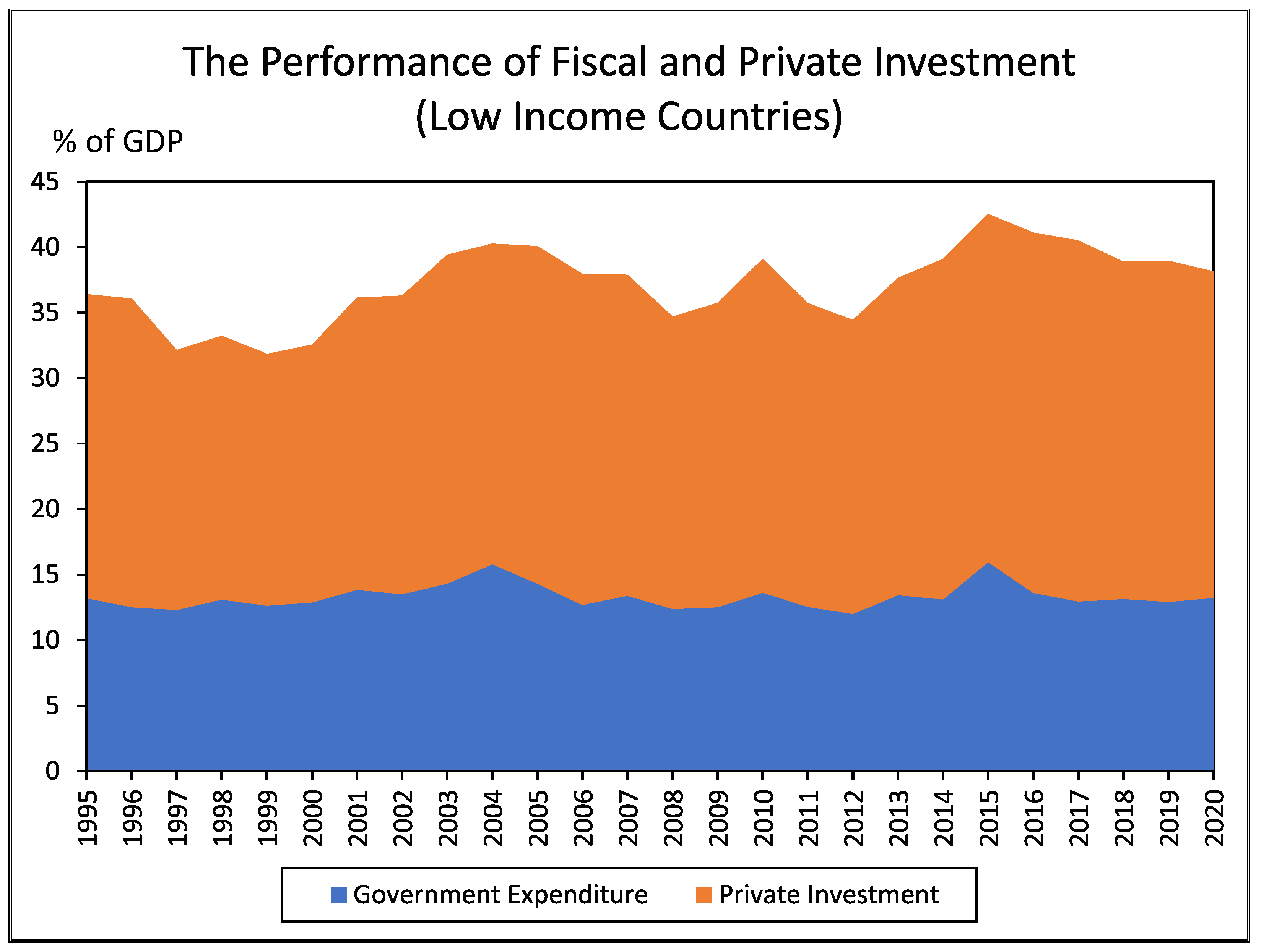
The ratios of government expenditure to GDP and of private investment to GDP for developing countries are plotted in Figure 1 and Figure 2. These are divided according to the level of income, namely low-income countries and middle-income countries. Preliminary examination may suggest that the crowding out effect is supported by data. These trends however do not indicate whether the existence of crowding out effect is caused by government expenditure. This is due mainly to the inconsistent relationship in the theory between government expenditure and private investment during the period of study. Hence, further studies need to be conducted to obtain conclusive results. Furthermore, the existing empirical studies concerning this problem have also produced mixed results. This study is therefore necessary to identify the existence of the crowding out effect in order to determine the effectiveness of fiscal policy.

4. Methodology

4.1. Data

The study utilized the annual data from 1990 to 2020 for the sample of 60 developing countries (Appendix A). The data set were collected from various sources such as the IMF International Financial Statistics (IFS), Government Financial Statistics (GFS), Asian Development Bank—Key Indicators for Asia and the Pacific, World Bank, World Development Indicators and the website of the Department of Statistics and the Central Banks from developing countries. All variables such as defense expenditure (LGDEF), economic expenditure (LGECO), social expenditure (LGSOC), private investment (LPI) and private consumption (LPC) were transformed into log form except for interest rate (INT) and trade openness (OPN), which were indicated in percentage points.
This study examines the effects of fiscal policy on private expenditure using a panel VAR for the sample of 60 developing countries from 1990 to 2020.

4.2. The Specification Panel Var (PVAR) Model

A panel data vector autoregression methodology was used to estimate the effect of fiscal policy on private expenditure. Generally, PVAR has the same structure as VAR models, which treats all variables in the system as endogenous and interdependent, both in a dynamic and in a static sense. Let Y t be a G × 1 vector of endogenous variables. The VAR for Y t is
  Y t = Г 0 + Г 1 Y , t 1 + ε t
where Г 1 is a polynomial in the lag operator and ε t means identically and independently distributed. Panel VAR have the same structure as VAR models but there were significant differences between VAR and PVAR models in the use of cross-sectional data. Accordingly, Y t the vector in the VAR model was replaced with Y i t in the PVAR model. The vector for each unit i = 1 , , N , i.e., Y t = ( y 1 t ,   y 2 t , . y N t ) . The index i is generic and could indicate countries, sectors, markets or their combination. In this study, i represents the country.
The dynamic relationship between fiscal policy and macroeconomic variables in the PVAR model is as follows:
  Y i t = Г 0 + Г 1 Y i , t 1 + f i + d c , t + ε i t
where, Y i t is a vector of endogenous variables consisting of eight variables (INT, LPI, LPC, OPN, LDY and government expenditure variables, LGDEF, LGECO and LGSOC), while Г 0 is a constant vector and ε i t is error vector for state i . in period t .
The VAR panel model framework was used to focus on the disaggregated government expenditures which included the defense, economic and social expenditure. To detail out the analysis, the composition of government spending was divided into two, namely productive expenditures and non-productive expenditures. Therefore, we derived six models which contain one of the compositions of government expenditure (LGDEF, LGECO and LGSOC) and private expenditure (LPI and LPC). The structure model can be written as follows:
Model   1 :   Y i t = ( O P N i t , I N T i t , L G D E F i t ,   L P I i t , , L D Y i t ) Model   2 :   Y i t = ( O P N i t , I N T i t , L G E C O i t , L P I i t , , L D Y i t ) Model   3 :   Y i t = ( O P N i t , I N T i t , L G S O C i t , , L P I i t , L D Y i t ) Model   4 :   Y i t = ( O P N i t , I N T i t L G D E F i t , L P C i t , , L D Y i t ) Model   5 :   Y i t = ( O P N i t , I N T i t L G E C O i t , L P C i t , , L D Y i t ) Model   6 :   Y i t = ( O P N i t , I N T i t , L G S O C i t , , L P C i t , L D Y i t )
Based on the six models, we have ordered all the variables based on the economic theory. For the first variable is trade openness. Trade openness is describing the country in open economic activities. The justification is supported by Ahmed et al. [20] was stated the variable of trade openness can influence investment decisions. According to economic theory, the lack of trade openness retard economic growth. From the above reason, trade openness is placed in the first position. Through the recursive identification approach, it is assumed that trade openness (OPN) is exogenous to other variables such as interest rate (INT), government expenditure (LGDEF, LGECO and LGSOC), private investment (LPI), private consumption (LPC) and domestic (LDY). OPN is considered an exogenous variable that does not respond immediately or showed lags in the movement of the endogenous variables.
Next is INT which is in the second position. This is considered reasonable as it is assumed that the monetary policy implementation is not immediately affected by other variables which include LGDEF, LGSOC, LGECO, LPI, LPC and LDY. This justification is supported by previous literature such as Bernake and Blinder [27], Bernanke and Minhov [28] and Christiano et al. [29].
Government expenditure such as LGDEF, LGECO and LGSOC was assumed to respond contemporaneously to the OPN. The relationship between government expenditure and OPN is assumed to be positive. This justification is supported by the compensating hypothesis proposed by Rodrik [30]. According to the hypothesis, an increase in trade openness may increase the size of government in the form of redistributive public expenditure to offset for increasing risk caused by possible international market turbulence. In this connection, the government sector is seen as safe, in terms of employment and income thereby making it easier to isolate its function over external risks by increasing its impact on the entire economy.
LPI and LPC were assumed to respond contemporaneously to interest rates, government expenditure and trade openness. The theory of classic economics assumes that private investment and private consumption are influenced by interest rates and the relationship is negative. The justification for private expenditure is consistent with that of a previous study such as by Levine et al. [31]. The authors showed that only trade openness could firmly influence the investment. This suggests that the increase in trade openness can lead to greater investment either through internal or external sources.
LDY was placed at the last position and assumed an endogenous variable, suggesting that it responded immediately to all the variables such as INT, LGDEF, LGECO, LGSOC, LPI, LPC and OPN. This assumption is reasonable because LDY is a fast-moving variable in the system. According to Keynesian theory, national income is influenced by private spending (private investment and private consumption) and government spending. According to the economic theory, trade openness can rapidly influence economic growth of the country. Based on the comparative advantage theory, a country has a comparative advantage if it can produce goods at a lower opportunity cost than in another country. The low cost means that it has to forego less of other goods in order to produce it. This suggests that a country with comparative advantage will export the goods while a country without such comparative advantage will import the goods. Thus, trade openness through exports and imports is capable of stimulating economic growth.
The VAR panel analysis followed the methodology of Love et al. [32]. The authors stated the need to impose restrictions that the underlying structure is the same for each cross-sectional unit. This constraint is likely to be violated in practice. One way to overcome the restrictions on parameters is to allow for “individual heterogeneity” at the variables level by introducing a fixed effect, denoted as f i in the model. However, it is seen that the fixed effects are correlated with the regressors due to lags of dependent variables and the mean-differencing procedure used to eliminate fixed effects would create biased coefficient. To avoid this problem, we used forward mean differencing, also referred to as the ‘Helmert procedure’. This procedure removes only the forward mean, such as the mean of all the future observations available for each country-year. This transformation preserves the orthogonality between transformed variable and lagged regressor. We can therefore use lagged regressor as an instrument and estimate the coefficients using the GMM (general method of moments) system.
This model also includes country-specific time dummies d c , t as shown in Equation (1) to capture aggregate, country-specific macro shocks that may affect all countries in the same way. We eliminated these dummies by subtracting the mean of each variable calculated for each country-year.
In order to analyze the impulse response functions, the confidence intervals need to be estimated. Since the matrix of impulse response functions is constructed from the estimated VAR coefficients, the standard errors need to be considered. The standard error of the impulse response functions needs to calculate and generate confidence intervals through the Monte Carlo simulation. Finally, the variance decompositions analysis is also described in the empirical results that indicate the percent of the variation in one variable that is explained by the shock to another variable, accumulated over time. The variance decompositions show the magnitude of the total effect and report the total accumulated effect over 10 years. However, it was found that longer horizons produce equivalent results.

5. Empirical Results

5.1. Estimation of Coefficients

We estimated the coefficient of the system given in (1) after the fixed effects and the country-time dummy variable have been removed. In Table 1, we report the results of the disaggregated government expenditure on private investment, while in Table 2, we report the results of the disaggregated government expenditure on private consumption.
Panel A in Table 1 presents the defense expenditure. The results show that a positive shock of defense expenditure has a significant positive relationship on interest rates and national income at 1% and 10% significance level, respectively, while the response to private investment shows insignificant results. However, the relationship between defense expenditure and private investment is negative. Panel B describes the coefficient of economic expenditure. The results indicate that the shock of economic expenditure led to a significant positive relationship on interest rates, private investment and national income at the 1% and 10% significance level. Panel C presents the social expenditure. It is clear the results show a positive relationship in private investment with national income and significant at the 1% level.
Panel A in Table 2 presents the defense expenditure. The positive shock of defense expenditure is positively significant to interest rates and national income at the 1% and 10% level, respectively. Panel B shows a positive relationship among economic expense to interest rates, private consumption and national income at the 1% and 5% significance level. And panel C presents social expenditure. The estimation of coefficient shows that national income has a positive relationship with social expenditure at a 1% significance level.

5.2. Impulse Response Function

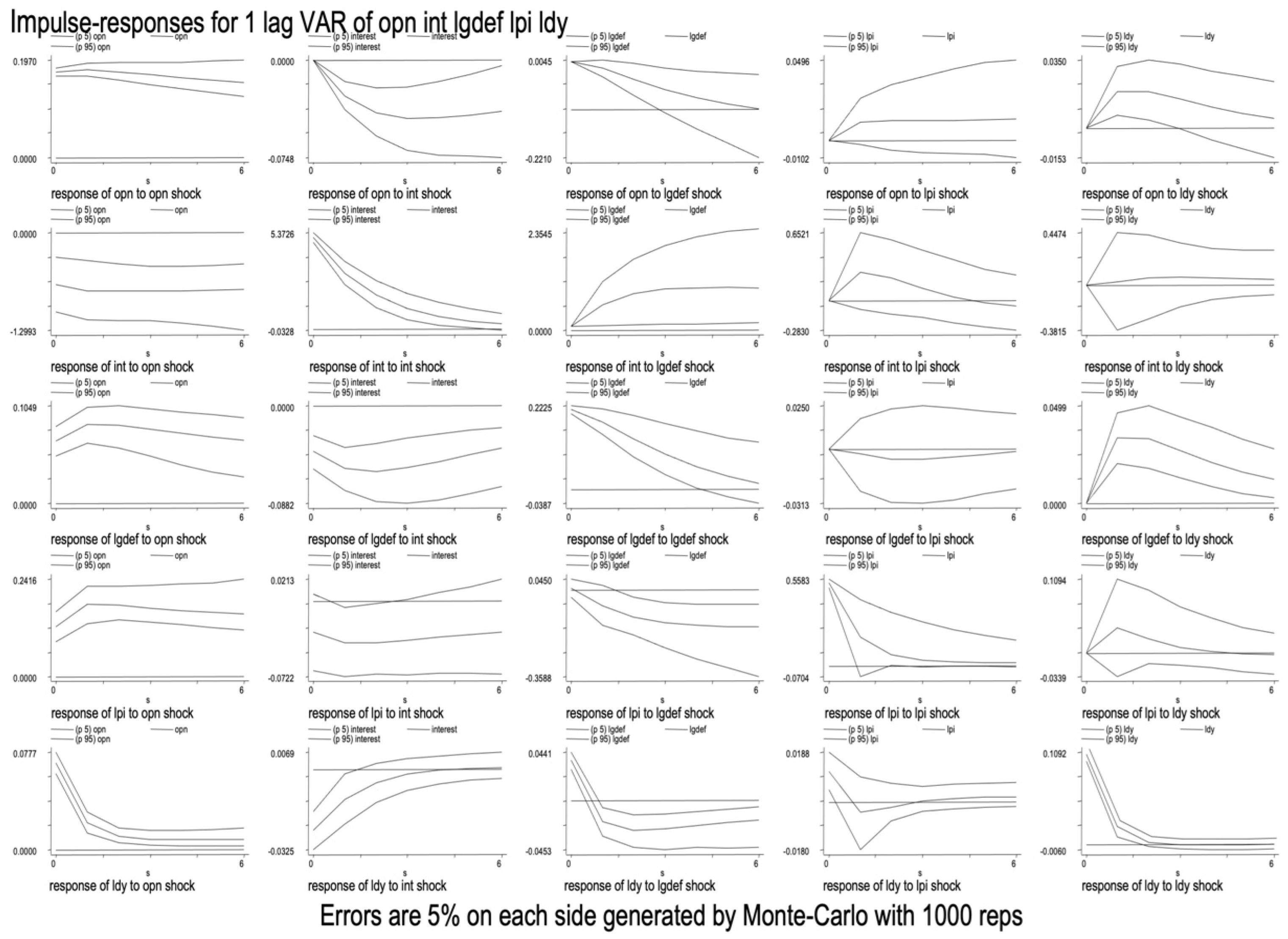
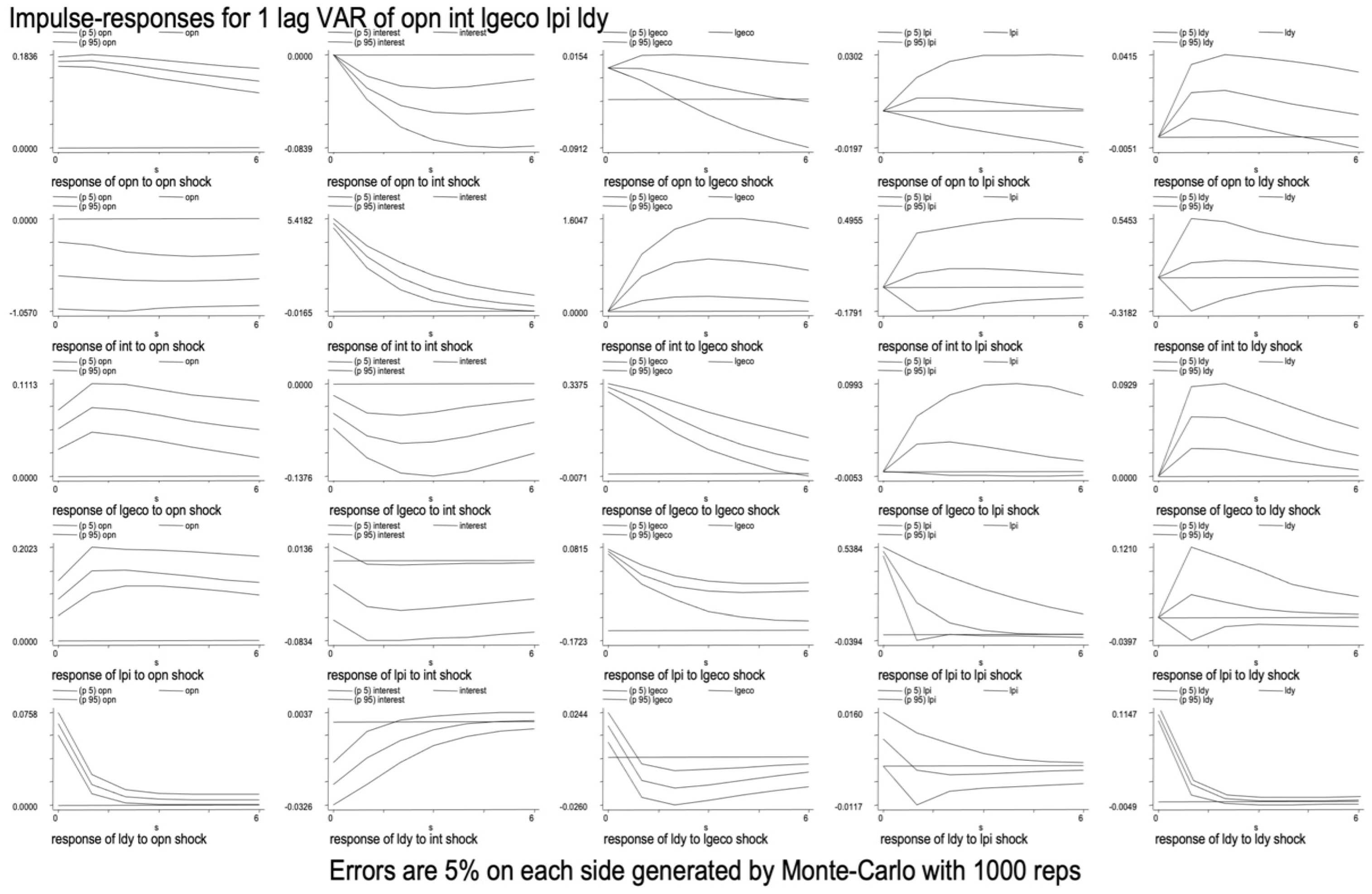
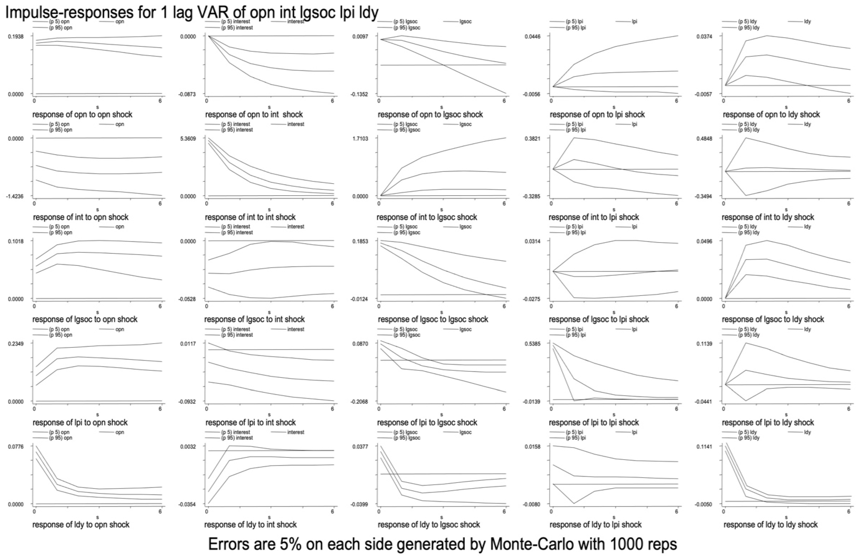
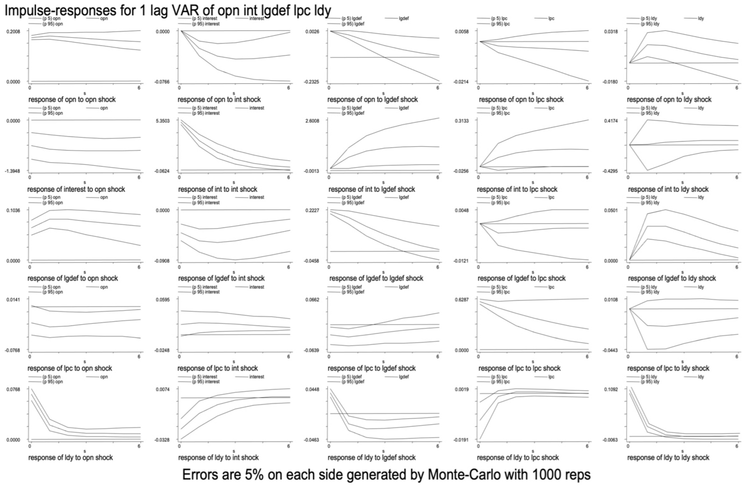
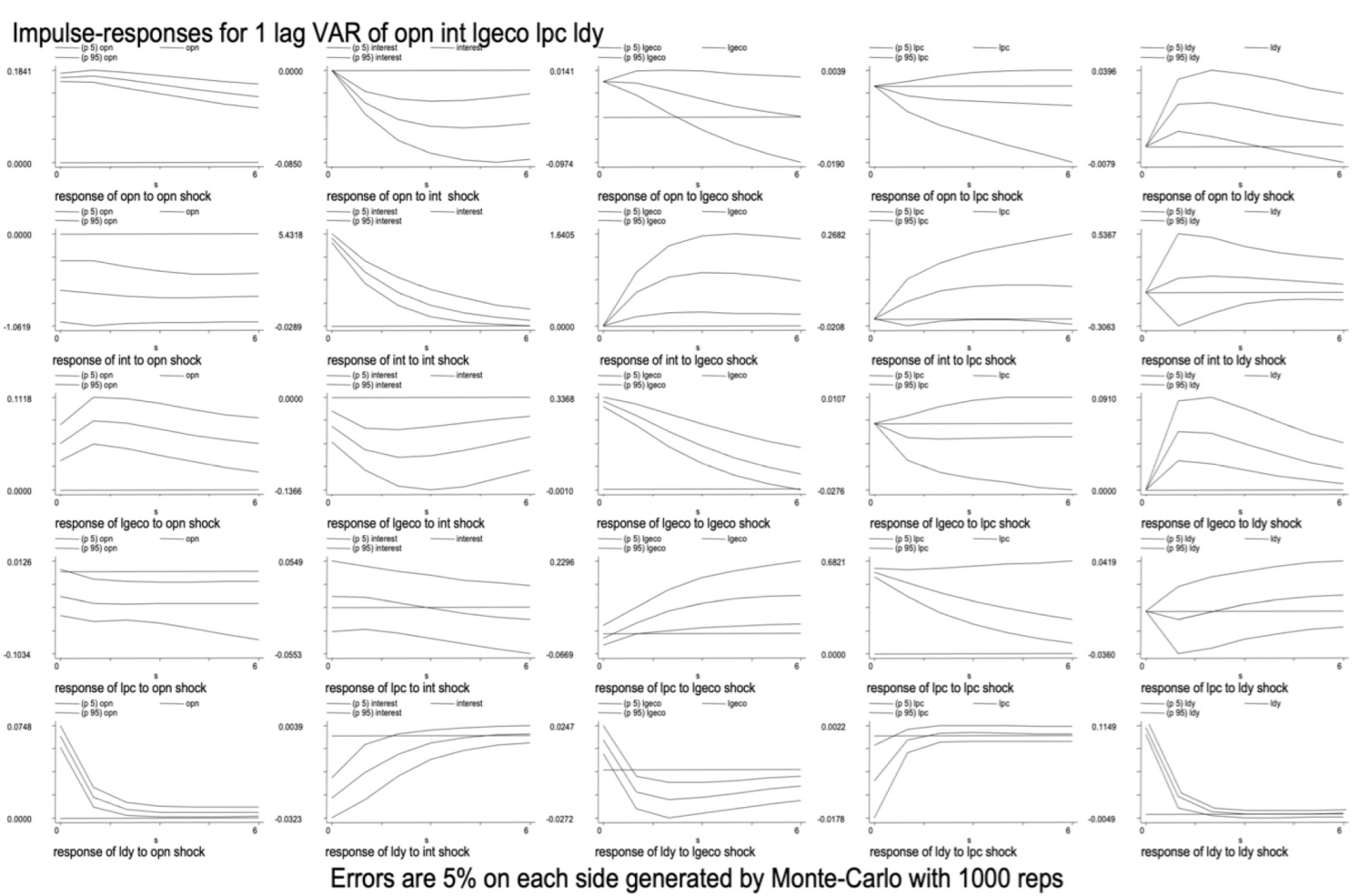
Figure 3, Figure 4, Figure 5, Figure 6, Figure 7 and Figure 8 illustrate the impulse response function of the endogenous variable in this study. The main focus of this analysis was to examine the effect of disaggregated government spending, such as defense, economic and social spending, on private expenditure. Additionally, the analysis also included macroeconomic variables such as interest rates, domestic income and trade openness. The solid line in the center represents the estimated responses, whereas the solid line between the middle solid lines represents confidence intervals which have the upper boundary line representing 95% confidence interval and the bottom boundary line represents 5% confidence interval as derived from Monte Carlo simulation and bootstrapped 1000 times. The significance of the impulse response functions was based on the upper bound lines and the lower bound lines. This shows that the impulse response functions are significant if the upper boundary and lower boundary lines are in one direction, either positive or negative. Conversely, if the upper boundary lines and the lower boundary lines show opposite directions (for example the upper boundary line is positive and the lower boundary line is negative), then the impulse response functions are considered insignificant.

5.3. The Disaggregated Government Expenditure on Private Investment and Macroeconomic Variables

5.3.1. Defense Expenditure

Figure 3 shows the impulse response function of the defense expenditure on private investment and other macroeconomic variables. As can be seen in Figure 3, the positive shock of the defense spending to interest rates is significant and positive. This response is consistent with the estimation coefficients result which shows that the increase in defense expenditure leads to an increase in interest rates.
The response of private investment to defense expenditure shocks is significantly negative which indicates that defense expenditure creates crowding out effects on private investment. The response is also consistent with the classical theory where increases in government spending financed by bonds may lead to an increase in the demand for loanable funds. This situation thus creates excess in supply which thus causes interest rates to rise. This would subsequently create two effects: firstly, an increase in savings and secondly, reduction in private investment. The finding is also consistent with Malizard [33] who found that military spending crowds out private investment.
The national income responded positively to the defense expenditure shock at the beginning of the study period. However, the positive response of national income began to reduce and become negative in the midterm. This finding is consistent with the private investment response which creates the crowding out effect. The results also support the classical analysis which indicates that increase in government spending creates the crowding out effect on private investment that will finally tend to reduce national income.

5.3.2. Economic Expenditure

Figure 4 indicates the effect of economic expenditure on private investment and other macroeconomic variables. The positive shock of economic expenditure responded positively to the interest rate. The positive response of interest rate to economic expenditure can be explained by Keynesian theory, which indicates that an increase in government expenditure increases the interest rate. This mechanism is initiated with an increase in government spending which subsequently stimulates national income and an increase in the demand of money for transactions. If money supply is fixed, the public will sell bonds for cash thus leading to reduction in bond demand. Overall, increasing the demand for money and reducing the demand for bonds lead to reduced bond prices and an increase in interest rates.
Private investment responded positively to economic expenditure which suggests that the positive shock due to the latter creates the crowding in effect on the former. This response is consistent with the coefficient results which showed a positive relationship between economic expenditure and private investment.
Response in national income was positive to economic expenditure at the beginning of the period suggesting that an increase in economic spending led to an increase in domestic income. However, in the midterm, this response gradually reduced to a negative value thus indicating that the reduction in national income was due to the effect of economic expenditure shock.

5.3.3. Social Expenditure

Figure 5 presents the effect of social expenditure on private investment and other macroeconomic variables. The interest rate has responded positively to the social expenditure shocks. The result indicates that an increase in social expenditure stimulated interest rates, a response that is consistent with Keynesian theory.
Private investment responded positively to the positive innovation in social expenditure thus indicating the existence of a crowding in effect. This response is consistent with result in estimation of coefficients. However, in mid-period the response began to decrease and became insignificant.
The response of national income to the positive shock of social expenditure was significant and positive at the beginning of the period. This suggests that the increase in social expenditure caused the national income to rise. The response is consistent with private investment that exerts a positive impact as a result of the increase in social expenditure. This response was however negative at midterm, thus indicating the existence of a crowding out effect in national income.

5.4. The Disaggregated Government Expenditure on Private Consumption and Macroeconomic Variables

5.4.1. Defense Expenditure

Figure 6 shows the effect of defense expenditure shock on private consumption and other macroeconomic variables. The interest rate responds positively to the defense expenditure shock indicating that the increase in defense expenditure leads to increase in interest rates.
Private consumption responds significantly and positively to the defense expenditure shock, which suggests the existence of the crowding out effect in private consumption. The finding is also consistent with those of previous studies such as in Ismail et al. [26], where current expenditure for defense showed a negative relationship with private consumption. This response, which is consistent with the private investment response, also suggests the existence of crowding out effect.
The response of national income to the innovation in defense expenditure was positive at the beginning of the period. However, in the mid-period, the response began to decrease to negative values. This indicates that the impact of crowding out has no effect on aggregate demand even though government expenditure is increased. Since the expansion of government expenditure has no effect on aggregate demand, its increase through bond sales has also no effect on price level. Overall, the expansion of fiscal policy has no effect on the aggregate demand and national income.

5.4.2. Economic Expenditure

Figure 7 presents the impulse response function of economic expenditure on private consumption and other macroeconomic variables. The response in interest rate to economic expenditure shock is significant and positive. This suggests that the expansion of fiscal policy through increased government expenditure leads to increases in the interest rate. The result is consistent with Keynes and classical theory.
Private consumption responds positively and significantly to the shock in economic expenditure. In other words, the relationship between private consumption and economic expenditure is complementary, thus indicating that the positive response in consumption creates a crowding in effect. The response is also consistent with the estimation coefficients, suggesting a significant positive response between economic expenditure and private consumption as well. The result is also consistent with those of previous studies such as Ismail et al. [26] who found that economic expenditure, as in the agricultural sector, showed a positive effect on private consumption.
A positive shock in economic expenditure caused the national income to respond at the beginning of the period. This response is consistent with those for interest rates and private consumption, which showed a positive relationship. The results also supported the Keynesian analyses, which indicate that fiscal policy is an effective tool for boosting sustainable economic growth.

5.4.3. Social Expenditure

Figure 8 describes the impulse response function of social expenditure to private consumption and other macroeconomic variables. The response of interest to the innovation in social expenditure is positive.
The private consumption response was found to be consistent with response in the interest rate which showed a positive result. The social expenditure shock has created crowding in effect on private consumption. The results are consistent with those of prior studies such as by Marattin et al. [34], who examined government spending on private consumption and investment in 14 European Union countries comprising Austria, Belgium, Denmark, Finland, France, Ireland, Italy, Germany, Greece, the Netherlands, Portugal, Spain, Sweden and the United Kingdom for the period 1970 to 2006. Public spending was shown to exert a positive impact on private consumption and private investment.
The national income has responded positively to the social expenditure shock. This response is consistent with that for private consumption with both displaying a positive relationship.

5.5. Variance Decomposition

5.5.1. Variance Decompositions for Disaggregated Government Expenditure on Private Investment

Table 3 presents the analysis of variance decomposition for disaggregated government expenditures such as defense, economic and social areas on private investment. Panel A presents defense expenditure that indicates the period of variation which occurs in 10 periods ahead. Estimated contribution to variations of changes in LGDEF comprised 9.5% by itself and 1.9% by OPN. The private expenditure component, such as LPI, contributed about 0.5%.
Panel B presents economic expenditure. For the 10 periods ahead, the innovation of changes in LGECO is about 9.4% from itself. The finding indicates that the economic expenditure shock is mainly due to LGECO itself. The remaining contributions are due to LPI and LDY for about 0.9% and 0.6% respectively, with INT and OPN as the smallest contributors at about 0.5%.
Panel C shows variation in social expenditure in the 10 periods where it contributed the largest spending at around 9.1%. The remaining was attributed to other variables which included OPN for 0.3%, INT around 0.2%, LPI about 0.9%, with LPI being the smallest at 0.8%. The analysis of variance decomposition indicates that government expenditure, which includes defense, economic and social expenditure, is not the major or largest contributor to private investment.

5.5.2. Variance Decompositions for Disaggregated Government Expenditure on Private Consumption

Table 4 presents the analysis of variance decomposition for disaggregated government expenditure on private consumption. Panel A shows the defense expenditure. The innovation of changes in LGDEF by itself contributed around 9.5% in the 10 periods ahead. The second largest is LPC with about 0.8% and the smallest contributor LDY at around 0.6%.
Panel B presents the economic expenditure. The variation of changes is mainly contributed by itself which accounts for 9.5%. The second largest is LPC with about 2.3%. The remaining percent is attributed to INT for about 0.3%, OPN for 1% and LDY around 0.7%.
Panel C presents the social expenditure. The positive shock in social spending for the 10 periods was mainly due to itself with the largest contribution of around 4.1%. The second largest contribution was by LPC, accounting for 3.6%, and the third largest contributor was by LDY at around 2.5%.
Based on the variance decomposition analysis private consumption contributed a small percentage of the innovation of changes in government expenditure such as those for defense, economic and social areas.

6. Robustness Checking

For robustness checking, alternative procedures were considered in this study such as the use of a model without monetary policy.

Model without Monetary Policy

The baseline model used the monetary policy variable which is the interest rate offsetting the effect of fiscal policy expansion. Since the main purpose of this research is to study the impact of fiscal policy shocks, it is assumed that the model is without a monetary policy variable. The results of the analysis found that the impulse response function of the effect of fiscal policy, which is defense spending shocks, economic spending and social spending on private investment, private consumption and domestic income in NSM, is almost the same in the baseline model. Overall, the impulse response function, with baseline restriction, was found to be robust.

7. Conclusions

In this study, the effect of a fiscal policy shock on private spending in developing countries was examined. The VAR panel model framework was used to focus on the disaggregated government expenditures which included defense, economic and social areas. They either created the crowding out effect or crowding in effect on private expenditure. To detail out the analysis, the composition of government spending was divided into two, namely, productive expenditures and non-productive expenditures. This suggests that the composition of government expenditure is classified as productive expenditure if the effects of the response created a crowding in effect on private expenditure, or as non-productive expenditure, if the effect of the response created a crowding out effect on such expenditure.
An empirical study should more accurately and specifically estimate government spending to explain the relationship and the resulting rewards on private spending. Several conclusions can be drawn from the results. Firstly, the positive shock of defense expenditure on private spending, such as in private investment and private consumption, was found to elicit negative effects. This should suggest that an increase in government spending on defense would lead to a decrease in private investment and private consumption. The same is true for national income, which showed a negative effect in the mid-period. Based on the findings, it is clear that defense expenditure is a non-productive expenditure since its increase affects the reduction in private spending in national income.
Secondly, the result indicated that an increase in economic expenditure produced positive effects on private investment, private consumption and national income. Government increases in economic expenditure, such as spending on the agriculture sector, forestry, fisheries and wildlife, energy and oil, mining, manufacturing and construction, transportation and communications, may stimulate private spending and domestic income. The existence of crowding in effects on private expenditure and domestic income shows that economic expenditure is a productive expense as it can improve economic performance and growth.
Thirdly, the positive shock of social expenditure on private investment, private consumption and national income also elicited positive response. This suggests that an increase in social spending may stimulate an increase in private investment, private consumption and national income. The findings show that social expenditure is a productive expense as it seeks to stimulate private spending increases such as private investment and private consumption, hence ultimately boosting economic growth.
Based on the findings, defense expenditure is thus classified as a non-productive expense since it does not stimulate an increase in private spending and national income whereas economic expenditure and social expenditure are considered productive expenses with the ability to stimulate economic growth and private spending. In this context, it is strongly recommended that the government increases its expenditure according to the relevant sector or composition. The government should thus be able to identify the sectors or compositions that have greater potential, capacity and relevance in stimulating sustainable economic growth.

Author Contributions

Conceptualization, I.H.K.; data curation, I.H.K.; formal analysis, I.H.K.; methodology, I.H.K.; supervision, M.S.A.-R.; writing—original draft, I.H.K.; writing—review & editing, M.S.A.-R. All authors have read and agreed to the published version of the manuscript.

Funding

This research was funded by University Kebangsaan Malaysia through Research-University grant (GGPM-2021-061) and the APC was funded by University Kebangsaan Malaysia.

Institutional Review Board Statement

Not applicable.

Informed Consent Statement

Not applicable.

Data Availability Statement

Not applicable.

Conflicts of Interest

The authors declare no conflict of interest.

Appendix A

Table A1. List of 60 Developing Countries.
NoCountryNoCountry
1Afghanistan31Lithuania
2Albina32Madagascar
3Bangladesh33Malaysia
4Belarus34Mexico
5Belize35Moldova
6Bolivia36Mongolia
7Bostwana37Morocco
8Bulgaria38Myanmar
9Burundi39Namibia
10Cambodia40Nepal
11Cameroon41Pakistan
12Chile42Panama
13China43Papua
14Colombia44Filipina
15Egypt45Romania
16El-savador46Rusia
17Ethopia47Seychelles
18Fiji48Sri Lanka
19Georgia49Syria
20Ghana50Tajikistan
21Guatemala51Thailand
22India52Tunisia
23Indonesia53Uganda
24Iran54Ukraine
25Jamaica55Uruguay
26Jordon56Vanuatu
27Kenya57Venezuela
28Kyrgyz58Vietnam
29Latvia59Yemen
30Lebanon60Zambia
Table A2. Summary of Variables and Data Sources.
VariablesSources
Defense ExpenditureGovernment Financial Statistics (GFS), IMF and Key Indicators for Asia and the Pacific 2021, Asian Development Bank
Economic ExpenditureGovernment Financial Statistics (GFS), IMF
Social ExpenditureGovernment Financial Statistics (GFS), IMF
Trade OpennesCalculation for Trade Openness:
= X + M K D N K
Interest RateInternational Financial Statistics (IFS), IMF
National IncomeInternational Financial Statistics (IFS), IMF and World Development Indicators
Private InvestmentInternational Financial Statistics (IFS), IMF and World Development Indicators
Private ConsumptionInternational Financial Statistics (IFS), IMF and World Development Indicators

References

  1. Aschauer, D.A. Fiscal policy and aggregate demand. Am. Econ. Rev. 1985, 75, 117–128. [Google Scholar]
  2. Monadjemi, M.S. Fiscal policy and private investment expenditure: A study of Australia and the United States. Appl. Econ. 1993, 25, 143–148. [Google Scholar] [CrossRef]
  3. Aschauer, D.A. Does public capital crowd out private capital? J. Monet. Econ. 1989, 24, 171–188. [Google Scholar] [CrossRef]
  4. Erenburg, S.J.; Wohar, M.E. Public and private investment: Are there causal lingkage? J. Macroecon. 1995, 17, 1–30. [Google Scholar] [CrossRef]
  5. Bairam, E.; Ward, B. The externality effect of government expenditure on investment in OECD countries. Appl. Econ. 1993, 25, 711–716. [Google Scholar] [CrossRef]
  6. Karras, G. Government Spending and Private Consumption: Some International Evidence. J. Money Credit Bank. 1994, 26, 9. [Google Scholar] [CrossRef]
  7. Erenburg, S.J. The real effects of public investment on private investment: A rational expectations model. Appl. Econ. 1993, 25, 831–837. [Google Scholar] [CrossRef]
  8. Argimon, I.; Gonzalez-Paramo, J.M.; Roldan, J.M. Evidence of public spending crowding-out from a panel of OECD countries. Appl. Econ. 1997, 29, 1001–1010. [Google Scholar] [CrossRef]
  9. Sie, S.J.; Kueh, J.; Abdullah, M.A.; Mohamad, A.A. Impact of public spending on private investment in Malaysia: Crowding-in or crowding-out effect. Glob. Bus. Manag. Res. Int. J. 2021, 13, 28–34. [Google Scholar]
  10. Hussain, A.; Muhammad, S.D.; Akram, K.; Lal, I. Effectiveness of government expenditure crowding-in or crowding-out: Empirical evidence in case of Pakistan. Eur. J. Econ. Financ. Adm. Sci. 2009, 16, 136–142. [Google Scholar]
  11. Heppke-Falk, K.; Tenhofen, J.; Wolff, G. The macroeconomic effects of exogenous fiscal policy shocks in Germany: A disaggregated SVAR analysis. In Deutsche Bundesbank Discussion Paper; 2006; Available online: https://dx.doi.org/10.2139/ssrn.2785268 (accessed on 1 May 2022).
  12. Gali, J.; Lopez-Salido, J.D.; Valles, J. Understanding the effects of government spending on consumption. J. Eur. Econ. Assoc. 2007, 5, 227–270. [Google Scholar] [CrossRef]
  13. Afonso, A.; Sousa, R.M. The macroeconomic effects of fiscal policy in Portugal: A Bayesian SVAR analysis. Port. Econ. J. 2011, 10, 61–82. [Google Scholar] [CrossRef]
  14. Afonso, A.; Sousa, R.M. The macroeconomic effects of fiscal policy. Appl. Econ. 2011, 44, 4439–4454. [Google Scholar] [CrossRef] [Green Version]
  15. Yadav, S.; Upadhyay, V.; Sharma, S. Impact of fiscal policy shocks on the Indian economy. J. Appl. Econ. Res. 2012, 6, 415–444. [Google Scholar] [CrossRef]
  16. Wang, T.-P.; Shyu, S.H.-P.; Chou, H.-C. The impact of defense expenditure on economic productivity in OECD countries. Econ. Model. 2012, 29, 2104–2114. [Google Scholar] [CrossRef]
  17. Laopodis, N.T. Effects of government spending on private investment. Appl. Econ. 2001, 33, 1563–1577. [Google Scholar] [CrossRef]
  18. Miller, S.M.; Russek, F.S. Fiscal structure and economic growth. Econ. Inq. 1997, 35, 603–613. [Google Scholar] [CrossRef]
  19. Mahmoudzadeh, M.; Sadeghi, S.; Sadeghi, S. Fiscal spending and crowding out effect: A comparison between developed and developing countries. Inst. Econ. 2013, 5, 31–40. [Google Scholar]
  20. Ahmed, H.; Miller, S.M. Crowding-out and crowding-in effects of the components of government expenditure. Contemp. Econ. Policy 2000, 18, 124–133. [Google Scholar] [CrossRef]
  21. Wang, B. Effects of government expenditure on private investment: Canadian empirical evidence. Empir. Econ. 2005, 30, 493–504. [Google Scholar] [CrossRef]
  22. Barro, R. Government Spending in a Simple Model of Endogenous Growth. J. Political Econ. 1990, 998, S103–S125. [Google Scholar] [CrossRef]
  23. Serven, L. Does Public Capital Crowd Out Private Capital? Evidence from India; Working Paper; The World Bank: Washington, DC, USA, 1996. [Google Scholar]
  24. Xu, X.; Yan, Y. Does government investment crowd out private investment in China? J. Econ. Policy Reform 2014, 17, 1–12. [Google Scholar] [CrossRef]
  25. Asri, N.M.; Tahir, M.Z.M.; Endut, W. Komposisi perbelanjaan kerajaan dan pertumbuhan ekonomi: Kajian empirikal di Malaysia. J. Kemanus. 2010, 8, 23–45. [Google Scholar]
  26. Ismail, N.A.; Ismail, A.G.; Osman, Z. Dasar fiskal dan asakan keluar mengikut sub-sektor perbelanjaan kerajaan di Malaysia. J. Kemanus. 2011, 9, 1–16. [Google Scholar]
  27. Bernanke, B.S.; Blinder, A.S. The federal funds rate and the channels of monetary transmission. Am. Econ. Rev. 1992, 82, 901–921. [Google Scholar]
  28. Bernanke, B.S.; Minhov, I. The liquidity effect and long-run neutrality. In Carnegie-Rochester Conference Series on Public Policy; North-Holland: Amsterdam, The Netherlands, 1998; pp. 49–100. [Google Scholar]
  29. Christiano, L.J.; Eichenbaum, M.; Evans, C. Chapter 2 Monetary policy shocks: What have we learned and what end? In Handbook of Macroeconomics; North-Holland: Amsterdam, The Netherlands, 1999; Volume 1, pp. 65–148. [Google Scholar]
  30. Rodrik, J. Why do more open economies have bigger governments? J. Polit. Econ. 1998, 106, 997–1032. [Google Scholar] [CrossRef]
  31. Levine, R.; Renelt, D. A sensitivity analysis of cross-country Growth Regression. Am. Econ. Rev. 1992, 82, 942–963. [Google Scholar]
  32. Love, I.; Zicchino, L. Financial development and dynamic investment behaviour: Evidence from panel VAR. Q. Rev. Econ. Finance 2006, 46, 190–210. [Google Scholar] [CrossRef]
  33. Malizard, J. Does military expenditure crowd out private investment? A disaggregated perspective for the case of France. Econ. Model. 2015, 46, 44–52. [Google Scholar] [CrossRef]
  34. Marattin, L.; Salotti, S. On the usefulness of government spending in the EU area. J. Socio-Econ. 2011, 40, 780–795. [Google Scholar] [CrossRef] [Green Version]
Figure 1. The performance of fiscal and private investment for low-income countries.
Sustainability 14 10786 g001
Figure 2. The performance of fiscal and private investment for middle-income countries.
Sustainability 14 10786 g002
Figure 3. Impulse response function for defense expenditure on private investment.
Sustainability 14 10786 g003
Figure 4. Impulse response function for economic expenditure on private investment.
Sustainability 14 10786 g004
Figure 5. Impulse response function for social expenditure on private investment.
Sustainability 14 10786 g005
Figure 6. Impulse response function for defense expenditure on private consumption.
Sustainability 14 10786 g006
Figure 7. Impulse response function for economic expenditure on private consumption.
Sustainability 14 10786 g007
Figure 8. Impulse response function for social expenditure on private consumption.
Sustainability 14 10786 g008
Table 1. The coefficients of disaggregated government expenditure on private investment.
Response ofResponse to
OPN ( t     1 ) INT ( t     1 ) LGDEF
( t     1 )
LPI ( t     1 ) LDY ( t     1 )
Panel A: Defense expenditure
OPN ( t ) 1.168
(5.00) *
−0.034
(−0.751) *
−0.123
(−1.24) *
0.025
(0.10)
0.404
(1.68) **
INT ( t ) −7.801
(−1.65) *
0.222
(1.18) *
0.031
(0.02) ***
6.177
(1.35)
8.380
(1.53)
LGDEF ( t ) 0.041
(0.32)
0.004
(0.190) ***
0.891
(12.76) *
−0.011
(−0.11)
0.109
(0.71) *
LPI ( t ) 0.082
(0.53) *
−0.004
(−1.43)
−0.385
(−0.53) **
0.934
(5.71)
0.209
(1.27)
LDY ( t ) 0.491
(1.88) *
−0.007
(−1.31) **
−0.164
(−1.47) *
−0.103
(−0.39)
0.045
(0.02) *
OPN ( t     1 ) INT ( t     1 ) LGECO
( t     1 )
LPI ( t     1 ) LDY ( t     1 )
Panel B: Economic expenditure
OPN ( t ) 1.268
(3.77) *
−0.005
(−0.83) *
−0.115
(−1.17)
0.138
(0.04)
0.540
(1.42) *
INT ( t ) −6.904
(−1.27) *
0.247
(1.34) *
0.550
(0.34) **
5.141
(0.97)
6.501
(1.01)
LGECO ( t ) 0.384
(0.93)
0.012
(1.47) ***
0.876
(7.08) *
0.355
(0.95) ***
0.540
(1.06) *
LPI ( t ) 0.142
(0.65) *
−0.003
(−0.73)
−0.020
(−0.32)
0.870
(3.89)
0.308
(1.26)
LDY ( t ) 0.642
(1.57) **
−0.109
(−1.26) ***
−0.131
(−1.02) *
−0.262
(−0.65)
0.248
(0.53) *
OPN ( t     1 ) INT ( t     1 ) LGSOC
( t     1 )
LPI ( t     1 ) LDY ( t     1 )
Panel C: Social expenditure
OPN ( t ) 1.245
(3.78) *
−0.004
(−0.78) *
−0.148
(−1.35)
0.129
(0.37)
0.409
(1.27) *
INT ( t ) −7.382
(−1.24) *
0.241
(1.26) *
0.937
(0.509) **
5.738
(0.96)
6.407
(0.98)
LGSOC ( t ) 0.022
(0.13)
0.001
(0.48)
0.914
(1.64) *
0.013
(0.09) ***
0.064
(0.34) *
LPI ( t ) 0.108
(0.51) *
−0.003
(−0.93)
−0.043
(0.59) **
0.898
(3.95)
0.212
(0.99)
LDY ( t ) 0.632
(1.58) *
−0.010
(−1.23)
−0.176
(−1.29) *
0.273
(0.67)
0.110
(0.26) *
Note: (*) denotes significance at the 1% level, (**) significance at 5% level and (***) significance at 10% level. t value is 2.58, 1.96 dan 1.64 for 1%, 5% dan 10% significance level, respectively.
Table 2. The coefficients of disaggregated government expenditure on private consumption.
Response ofResponse to
OPN ( t     1 ) INT ( t     1 ) LGDEF ( t     1 ) LPC ( t     1 ) LDY ( t     1 )
Panel A: Defense expenditure
OPN ( t ) 1.208
(6.27) *
−0.004
(−0.91) *
−0.178
(−1.16) **
−0.082
(−0.38)
0.562
(4.49) **
INT ( t ) −5.031
(−1.60) *
0.255
(1.55) *
0.575
(0.28) ***
6.667
(1.70) **
1.185
(0.52)
LGDEF ( t ) 0.032
(0.29)
0.007
(0.33) ***
0. 894
(9.58) *
0.027
(2.54)
0.111
(0.76) *
LPC ( t ) 0.152
(1.33)
0.002
(0.09)
−0.032
(−0.36)
0.786
(5.66) *
−0.193
(−1.84)
LDY ( t ) 0.514
(2.45) *
−0.008
(−1.49) **
−0.238
(−1.36) *
−0.057
(−0.22)
0.148
(1.01) *
OPN ( t     1 ) INT ( t     1 ) LGECO ( t     1 ) LPC ( t     1 ) LDY ( t     1 )
Panel B: Economic expenditure
OPN ( t ) 1.257
(5.67) *
−0.005
(−1.06) *
−0.144
(−1.21)
0.085
(0.27)
0.538
(4.73) *
INT ( t ) −4.515
(−1.36) *
0.279
(1.71) *
0.299
(0.19) *
4.734
(1.06) **
0.974
(0.47)
LGECO ( t ) 0.201
(0.98)
0.009
(1.91) **
0.840
(7.55) *
0.377
(1.20) *
0.773
(0.69) *
LPC ( t ) −0.162
(−1.22) ***
0.008
(0.26)
0.005
(0.08) ***
0.723
(3.79) *
0.189
(1.95)
LDY ( t ) 0.574
(2.34) *
−0.011
(−1.58) ***
−0.154
(−1.06) *
0.193
(0.59)
0.118
(0.83) *
OPN ( t     1 ) INT ( t     1 ) LGSOC ( t     1 ) LPC ( t     1 ) LDY ( t     1 )
Panel C: Social expenditure
OPN ( t ) 1.34
(4.14) *
−0.007
(−0.95) *
−0.272
(−1.42)
0.048
(0.13)
0.677
(3.07) *
INT ( t ) −5.375
(−1.26) *
0.259
(1.46) *
0.753
(0.33) **
4.964
(1.01)
2.231
(0.67)
LGSOC ( t ) 0.086
(0.68)
0.002
(0.93)
0.964
(1.24) *
0.051
(0.35)
0.202
(1.81) *
LPC ( t ) 0.169
(1.02)
−0.007
(−0.18)
−0.042
(−0.42)
0.782
(4.44) *
−0.211
(−1.46)
LDY ( t ) 0.687
(1.93) *
−0.012
(−1.40)
−0.309
(−1.32) *
0.053
(0.13)
0.306
(1.22) *
Note: (*) denotes significance at the 1% level, (**) significance at 5% level and (***) significance at 10% level. t value is 2.58, 1.96 dan 1.64 for 1%, 5% dan 10% signficance level, respectively.
Table 3. Variance decompositions for disaggregated government expenditure on private investment.
OPNINTLGDEFLPILDY
Panel A: Defense expenditure
OPN0.8130.0010.1870.0170.149
INT0.0080.8270.0770.0480.038
LGDEF0.0170.0300.9500.0090.009
LPI0.0320.0620.0540.8000.008
LDY0.0130.4630.0560.5590.325
OPNINTLGECOLPILDY
Panel B: Economic expenditure
OPN0.8110.00020.0490.0020.136
INT0.0030.7970.0470.0980.055
LGECO0.0130.0330.9380.0110.005
LPI0.0420.0590.0950.7430.061
LDY0.0200.0570.0640.5060.351
OPNINTLGSOCLPILDY
Panel C: Social expenditure
OPN0.8090.0020.0320.0140.143
INT0.0040.8540.0280.0670.046
LGSOC0.0300.0040.9090.08220.001
LPI0.0310.0500.0950.7560.067
LDY0.0200.0470.0860.4540.393
Note: The percentage of variation in the table is 10 periods ahead.
Table 4. Variance decompositions for disaggregate government expenditure on private consumption.
OPNINTLGDEFLPCLDY
Panel A: Defense expenditure
OPN0.7780.0060.0700.1470.004
INT0.0260.7850.0690.0600.061
LGDEF0.0130.0270.9460.0060.013
LPC0.0130.0420.0870.8390.019
LDY0.0430.0190.0630.4580.417
OPNINTLGECOLPCLDY
Panel B: Economic expenditure
OPN0.7960.0060.1340.0630.006
INT0.0030.8290.0340.0990.034
LGECO0.0110.0330.9500.0060.005
LPC0.0410.0420.2280.6800.009
LDY0.0280.0440.0750.3860.465
OPNINTLGSOCLPCLDY
Panel C: Social expenditure
OPN0.5340.0020.0360.4030.024
INT0.0350.8170.0520.0620.033
LGECO0.0480.0080.4110.3920.148
LPC0.1870.0020.3580.3870.067
LDY0.2060.0200.2480.2390.285
Note: The percentage of variation in the table is 10 periods ahead.
Publisher’s Note: MDPI stays neutral with regard to jurisdictional claims in published maps and institutional affiliations.