Article

A New Deep Learning Restricted Boltzmann Machine for Energy Consumption Forecasting

1
School of Economics, Fujian Normal University, Fuzhou 350007, China
2
National Key Project Laboratory, Jiangxi University of Engineering, Xinyu 338000, China
3
Vibrations and Acoustics Laboratory (VAL), Mechanical Engineering Department, Ozyegin University, Istanbul 34794, Turkey
4
Department of Computer Science and Artificial Intelligence, College of Computer Science and Engineering, University of Jeddah, Jeddah 23890, Saudi Arabia
5
Multidisciplinary Center for Infrastructure Engineering, Shenyang University of Technology, Shenyang 110870, China
6
Department of Earth Sciences, Sapienza University of Rome, Piazzale Aldo-Moro, 5, 00185 Rome, Italy
*
Author to whom correspondence should be addressed.
Sustainability 2022, 14(16), 10081; https://doi.org/10.3390/su141610081
Submission received: 27 July 2022 / Revised: 6 August 2022 / Accepted: 12 August 2022 / Published: 15 August 2022
(This article belongs to the Special Issue Artificial Intelligence and Sustainability)

Abstract

:
A key issue in the desired operation and development of power networks is the knowledge of load growth and electricity demand in the coming years. Mid-term load forecasting (MTLF) has an important rule in planning and optimal use of power systems. However, MTLF is a complicated problem, and a lot of uncertain factors and variables disturb the load consumption pattern. This paper presents a practical approach for MTLF. A new deep learning restricted Boltzmann machine (RBM) is proposed for modelling and forecasting energy consumption. The contrastive divergence algorithm is presented for tuning the parameters. All parameters of RBMs, the number of input variables, the type of inputs, and also the layer and neuron numbers are optimized. A statistical approach is suggested to determine the effective input variables. In addition to the climate variables, such as temperature and humidity, the effects of other variables such as economic factors are also investigated. Finally, using simulated and real-world data examples, it is shown that for one year ahead, the mean absolute percentage error (MAPE) for the load peak is less than 5%. Moreover, for the 24-h pattern forecasting, the mean of MAPE for all days is less than 5%.

1. Introduction

The most effective usage of power plants depends on many elements, such as weather variables like wind, humidity, and clouds, as well as other considerations such as holidays, months of the year, and days of the week. Due to its remarkable relevance for system operation and development, load forecasting has drawn considerable attention [1,2].
Proper load forecasting reduces investment costs and enables better planning for the construction of distribution and transmission networks. Electric loads are a dynamic, ever-changing characteristic. As a result, planning should be performed while considering reliability coefficients and the maximum load. Until future development, the planned network must also satisfy the demands of the area [3,4].
The load forecasting is classified into three levels: short-term, mid-term, and long-term. The applications and the methods of the three levels are different. At the short-term level, the forecasting horizon is just a few days, and it is used for short-term planning such as optimal use of power networks. Mid-term load forecasting (MTLF) denotes a monthly or, at most, annual forecast and is often used to manage peak consumption in certain seasons. The long-term level denotes the forecasting for some years ahead and is used for long-term planning, such as managing new power plants [5,6].
The remainder of this paper is organized as follows. Many different approaches for time series analysis and forecasting are reviewed in Section 2, and the main contributions of this study are listed at the end of this section. The effective variables are analysed in Section 3. In Section 4, the suggested RMB and the learning machine are described. The 24-h pattern forecasting and the forecasting of weekdays and weekends are studied in Section 5. In Section 6, the suggested application is described. Comparisons between MAPE and two different ANN-based methods are made in Section 7. Finally, the conclusions are given in Section 8.

2. Literature Review

MTLF helps to improve congestion planning in transmission networks, thus enhancing the system’s overall efficiency and optimizing energy costs for the consumer [7,8]. The advantage of exact MTLF is that companies can use it to improve their transmission network and distribution system. MTLF has been widely studied. In [9] investigated the economic impact of MTLF in the last two decades in market regulation and improvement of the transmission network and distribution system. Today, MTLF is also considered in energy transactions and assists in purchasing or selling energy and developing generation, transmission, and distribution contracts on a monthly or annual basis. It also affects the contractors of generators and distributors. Incorrect forecasts may lead to insufficient supply or oversupply. Therefore, it can be realized that exact MTLF leads to a more economical system [10].
The impact of climate conditions on the mid-term horizon has been comprehensively investigated in [11]. In [12], an MTLF scheme using the autonomous modelling technique is suggested to predict the monthly load, where the effective variables are only loaded and climatic variables. In this study, the authors compare the performance of the statistical method with the results of artificial intelligence and conclude that the method based on artificial intelligence yields better results. It has also been shown that statistical preprocessing is required for data analysis. In [13,14], an artificial neural network (ANN) approach is suggested that offers better results than statistical methods (regression models). In this reference, the forecasting of monthly load demand for one year is examined. In [15], an MTLF model based on a dynamic ANN is proposed. The model presented in this reference is compared with the statistical approach, and it is concluded that the values forecast by the proposed method are more accurate. The main advantage of the model proposed in this paper is that meteorological forecasts are not used. Climate variables rarely have accurate forecasts on a horizon of more than a week. In [16], an MTLF model based on the neural network approach is presented without any climatic information. The transformer models are suggested in [17,18] for load forecasting.
The deep learning methods, fuzzy systems and ANNs are widely used for modelling and forecasting problems [19,20,21]. In a few studies, these methods have also been applied to load forecasting. For example, a short-term forecasting scheme is designed in [22], and the effect of weather conditions is studied. In [23], the optimized ANNs by particle swarm optimization approach is suggested for MTLF, and by various examinations, the reduction of the number of input variables is studied. In [24], an ANN approach is developed, and the elimination of climate variables from the list of input factors is investigated. In addition, the effect of population growth is investigated by the designed ANN model. In [25], the days of the week are divided into three sections: early days of the week, middle days of the week and the weekend, and a separate model is proposed for each section. In [26], the days of the year are divided into 12 parts, and a neural network model is presented for each part. In some sources, the problem data are divided into winter and summer. In [27], genetic algorithm-optimized neural networks are used for medium-term forecasting. In [28], radial neural networks are used for modelling and forecasting. In the method proposed in this reference, neural network inputs include time (year, month, number of days of the month and days of the week), economic factors and temperature. The economic factor and temperature forecast must be available to forecast load at a specific time. Ghaderpour et al. [29,30] utilized the least-squares spectral and wavelet methods to approximate the seasonal cycles in the geodetic, climate and streamflow time series that can be used for forecasting. In [31], a comprehensive review is presented to inveigle the various models for energy consumption.
In most of the MTLF methods above, (1) the specific region is investigated, and the presented approach cannot be easily applied to other regions; (2) in some described MTLF methods, the computations are too heavy and cannot be applied to real-world problems; and (3) in the ANN-based methods, conventional learning schemes are used. Regarding the discussion above, a new deep learning approach is suggested for MTLF. The main contributions include:
  • A comprehensive analysis is presented to evaluate the effect of various factors, such as economics, climate and load pattern.
  • A deep learning approach based on RBMs and CD algorithm is presented that can be easily applied to a real-world problem with high dimensionality.
  • In addition to the weights, the structure of RBMs is also optimized.
  • In addition to the load peak, the suggested approach is extended to predict the 24-h load pattern.

3. Determining the Effective Variables

In this section, the effect of each variable on load forecasting is examined. The ANN inputs are altered in different scenarios, and the load peak forecasting error is compared to determine which set of inputs yields the best prediction result. The results of modelling and forecasting are depicted in different diagrams. After identifying the effective inputs, the structure (number of neurons) is also optimized. A summary of the scenarios is given as follows:
1
Load peak, gross domestic product (GDP), temperature peak and humidity percentage peak on a similar day in the past five years; the inflation rate in the past five years; type of day (working day or holiday).
2
Load peak, humidity percentage peak and temperature peak on a similar day in the past five years; type of day.
3
Load peak and the average temperature on a similar day in the past five years; type of day.
4
Load peak and temperature peak on a similar day in the past five years; type of day.
5
Load peak, temperature peak and minimum temperature on a similar day in the past five years; type of day.
6
Peak temperature on a similar day in the past five years; GDP and inflation rate in the past five years; type of day.
7
Average load peak, average peak temperature and peak temperature on a similar day in the past five years; type of day.
8
Load peak and average load peak on a similar month in the past five years.
9
Load peak, average load peak and temperature peak on a similar day in the past five years; average load peak and average temperature peak on a similar month in the past five years; type of day.
10
Load peak on a similar day in the past five years; average load peak on a similar month in the past five years; type of day.
11
Load peak on a similar day in the past five years; average temperature peak on a similar month in the past five years; type of day.
12
Load peak and temperature peak on a similar day in the past five years; average load peak and average temperature peak on a similar month in the past five years; type of day.
13
Load peak and temperature peak on a similar day in the past five years; average load peak, average temperature and average humidity peak on a similar month in the past five years; type of day.
14
Load peak on a similar day in the past five years divided by the average load peak of the same year; temperature peak on a similar day divided by the average temperature peak in the same month in the past five years; type of day.
15
GDP, number of subscribers (NOS), inflation rate and temperature peak in the past five years; type of day.
16
Load peak in the past five years; type of day.
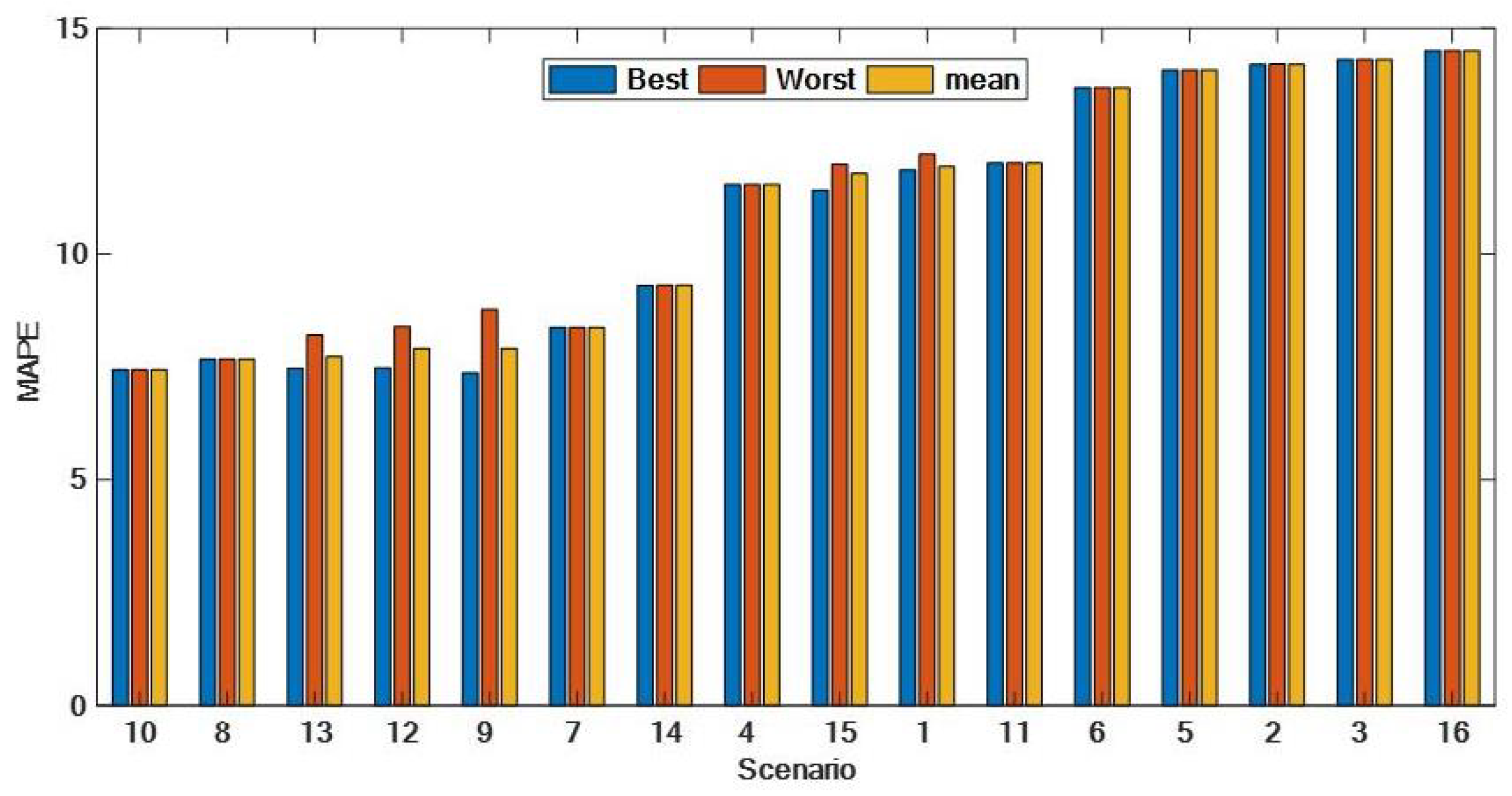
The deep learning algorithm is executed for all scenarios, and the results are given in Table 1 and Table 2. The desired results are acquired for a state where only climatic variables and historical load data are used. The MAPE diagram for test and training data sorted by the best average are illustrated in Figure 1 and Figure 2, respectively. For the entire validation data (one year and 7 months), the minimum MAPE is about 10%.

4. Suggested RBM and Learning Machine

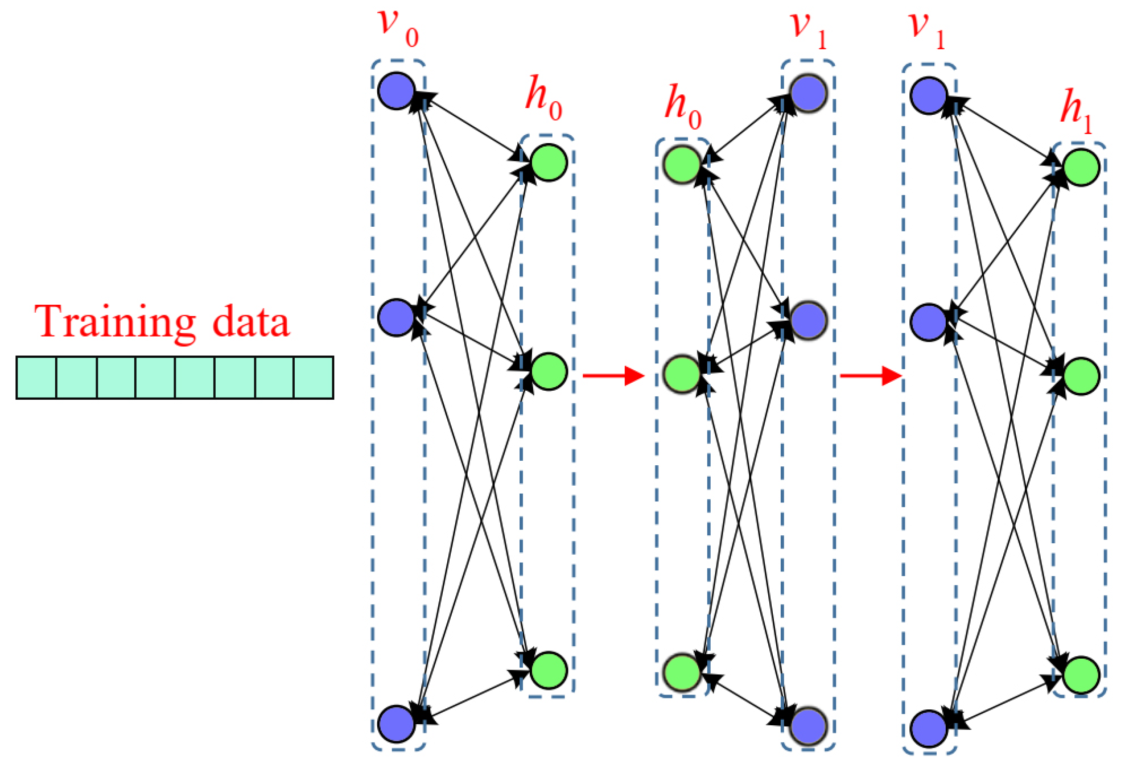
The proposed structure is displayed in Figure 3. The proposed algorithm for training is the contrastive divergence (CD) algorithm. The input variables are explained in the next section. The output of RBM represents the predicted load peak for the specified date. The suggested approach is also extended for 24-h pattern forecasting. The details of computing RBM and the learning method are given as follows:
(1) The degree of probability for apparent and hidden nodes is considered as follows.
p v k , h k , ξ , ε , δ = e E v k , h k , ξ , ε , δ k = 1 n E v k , h k , ξ , ε , δ ,
where ξ , ε , δ are trainable parameters, n is the number of training data segments, v k and h k are the input vectors in visible and hidden layers, respectively, and E is the cost function.
(2) The energy function is defined as follows [32]:
E v k , h k , ξ , ε , δ = h k T ξ v k ε T h k δ T v k .
(3) Initialization:
i t e r = 0 , Δ ξ = 0 n v × n h , Δ ε = 0 n h × 1 , Δ δ = 0 n v × 1 .
(4) For input data, v 0 , values of [ h 0 , v 1 , h 1 ] are obtained as follows:
h 0 = σ ξ T v 0 + ε v 1 = σ ξ h 0 + δ h 1 = σ ξ T v 1 + ε
σ x = 1 / 1 + exp x .
(5) Parameter changes are obtained using the following equations.
Δ ξ = γ Δ ξ + η n h 0 T v 0 h 1 T v 1
Δ ε = γ Δ ε + η n h 0 h 1 T 1 n × 1
Δ δ = γ Δ δ + η n v 0 v 1 T 1 n × 1
where γ and η are constant learning rates.
(6) Update the parameters using the following equations.
ξ t + 1 = ξ t + Δ ξ ς ξ t
ε t + 1 = ε t + Δ ε
δ t + 1 = δ t + Δ δ

5. Examining the Hourly, Weekdays and Weekends Forecasts

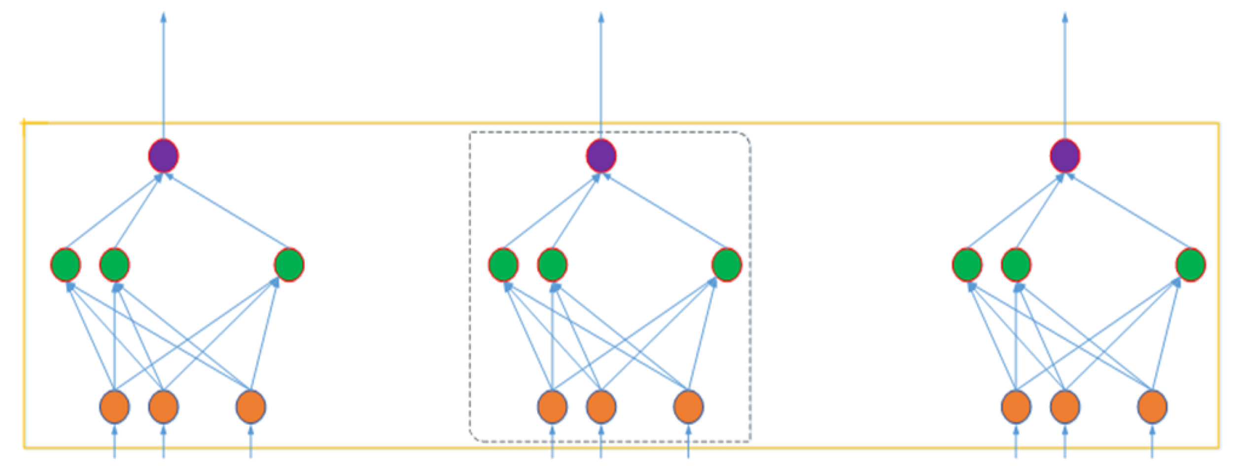
A local neural network is considered for each hour to enhance learning. The suggested structure is shown in Figure 4. The designed scheme leads to a better learning rate, while the effect of climatic information on some hours that are less temperature-dependent is decreased.
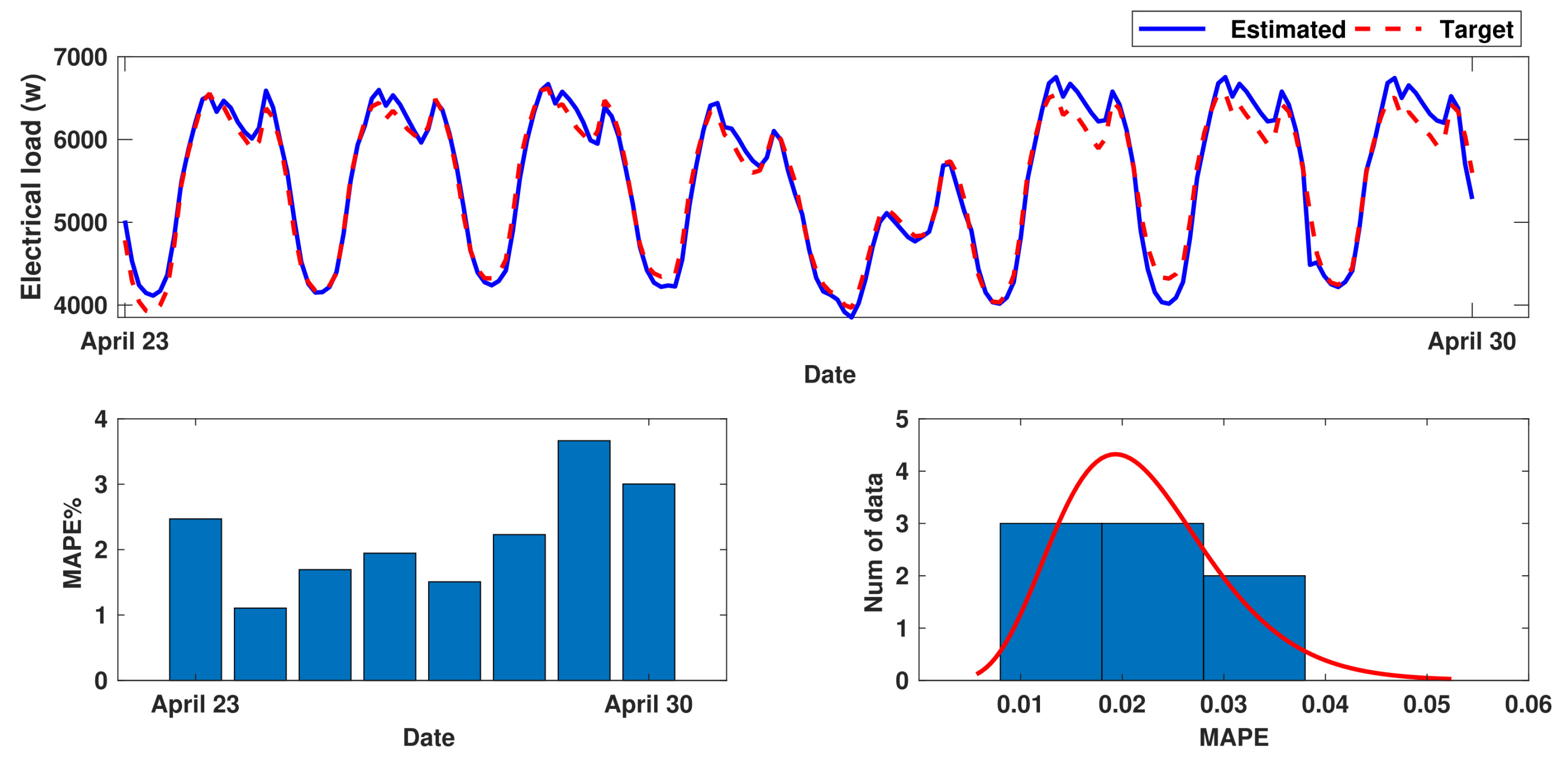
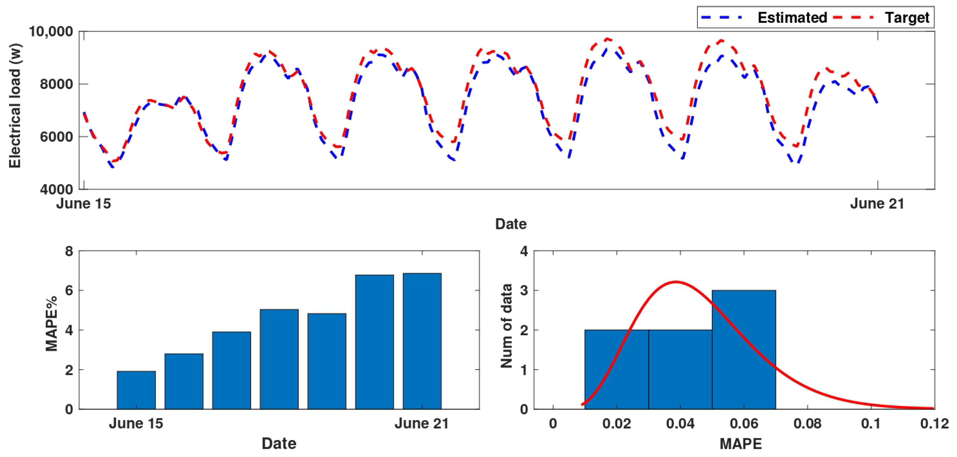
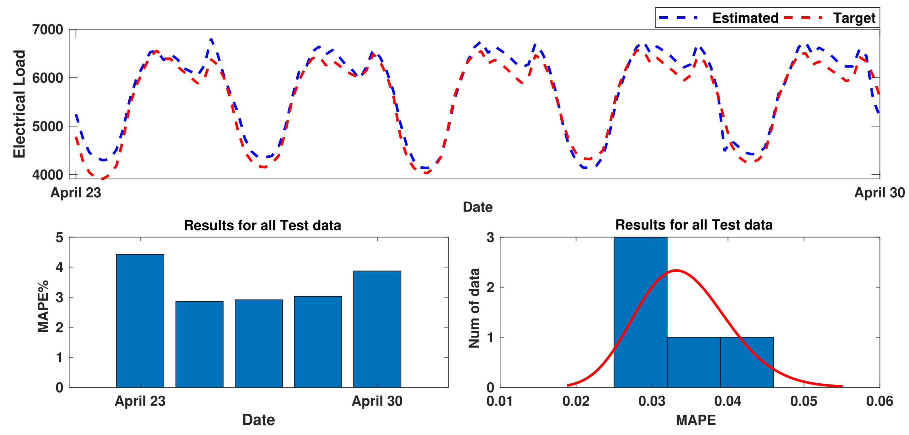
The proposed algorithm is generalized to hourly forecasting based on deep learning, similar to the previous section. Similar to Figure 3, a local RBM network is considered for each hour in the deep learning model. Load pattern forecasting for some weeks of April and June and their daily error percentage charts are shown in Figure 5 and Figure 6, respectively.
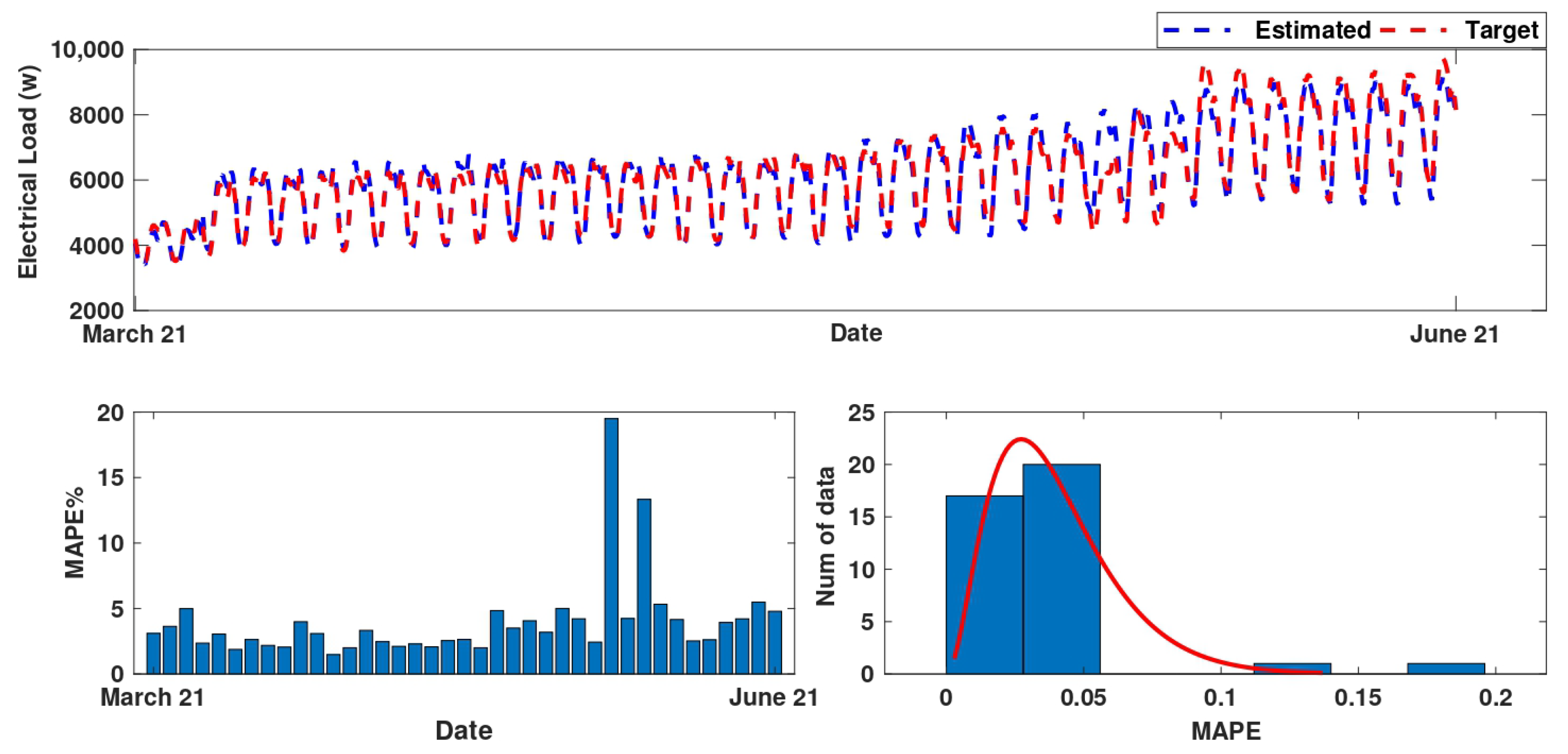
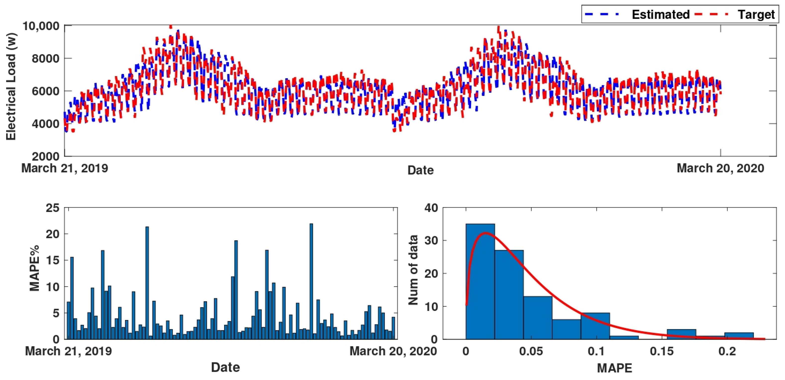
Similar to weekdays, the proposed algorithm based on deep learning is generalized to the holidays. In the suggested approach, the type of day is not considered as an input variable, but its effect is indirectly considered. In other words, the historical load data as the input variables are considered in similar days of past years. For evaluation, the data from March 2019 to March 2020 are used as the validation data and from March 2010 to March 2018 are used as the training data. Hourly forecast diagram for normal days in the first week of April 2019 and associated MAPE results are given in Figure 7. The hourly forecasts for normal days in spring 2019 and the related MAPE results are given in Figure 8. The hourly forecast diagram for holidays over a year, from March 2019 to March 2020, is shown in Figure 9. The load peak forecast chart for normal days during a year from March 2019 to March 2020 and the related MAPEs are illustrated in Figure 10. As the statistical analysis shows, for most days, the error rate is less than 5%.

6. Suggested Application

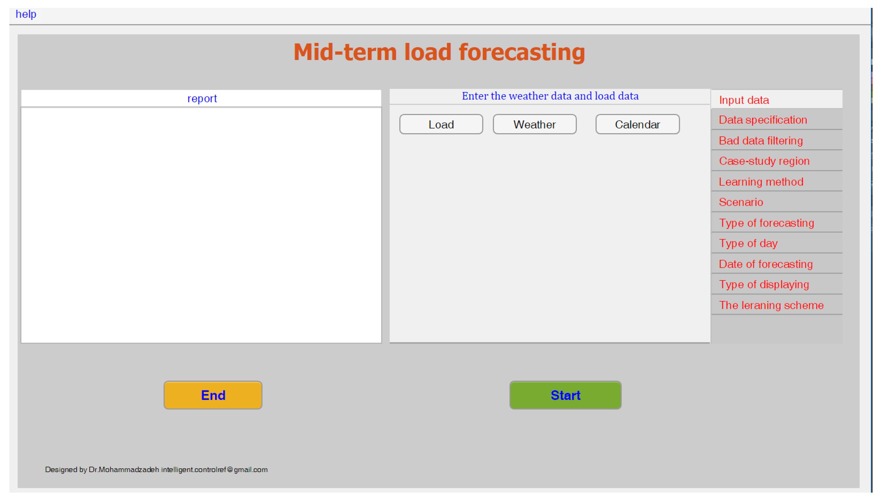
By various examinations, the most effective variables are considered to be the weather conditions, type of day and historical load data. A practical application is designed as shown in Figure 11. In this application, the type of inputs, the length of input data, the neurons and the layer number are optimized such that the most accurate performance is achieved. The main aspects of the designed scheme are summarized as:
  • Just the weather data, historical load data and calendar (a calendar which shows the type of days in the sense of working day or holiday) are considered as input data.
  • To consider the effect of other factors, such as economic factors and population, the case study region is classified into sub-regions. In addition, by considering the pattern of load consumption, the effects of some unavailable and uncertain factors are indirectly considered.
  • A simple algorithm is considered to find and correct the bad data. The data of each day are compared with the mean of similar days (similar days are defined as the days that are similar in the sense of working days or holidays, and they are not as far as one month). If the data of one day are far from the average, they are detected as a candidate for bad data. If the weather conditions of this candidate are closer to the mean of similar days, then they are considered bad data.
  • In addition to load peak forecasting, the 24-h pattern is also forecast for one year ahead.
  • To achieve the most accurate results, in addition to the parameters, the number of neurons, the number of layers, and the type of input variables are also optimized. It should be noted that, in the mid-term forecasting, various economic, social, and cultural factors are effective. Most of these factors are unavailable or uncertain. To consider the effect of these factors in an indirect scheme, the load data in the past dates are considered as input variables, and the length of historical data is optimized.
  • For a long period of prediction, to improve the accuracy, it is suggested that for each month, a different structure is optimized. The learning data is divided into some short periods, and for each period a different structure is optimized. For example, suppose that the period of prediction is from January to July one year ahead. The learning data are divided into seven parts, and for each month a different RBM is optimized.

7. Comparisons

In this section, some comparisons are given to better show the suggested approach’s superiority. In [13,16], the ANNs are applied to MTLF. The load peak forecast accuracy is examined for normal days during a year from March 2019 to March 2020. The values of MAPE are given in Table 3. The value of MAPE for the suggested method is remarkably better than conventional ANN-based approaches. In the proposed approach, the set of input variables, the number of layers in RBMs and the number of neurons are optimized to achieve the best accuracy. In addition, the parameters of hidden layers are well tuned by the suggested deep learning approach.

8. Conclusions

In this paper, an experimental approach based on deep learning techniques was designed for load forecasting. The proposed approach was applied to forecast the electrical load for the year ahead. In addition to optimizing the free parameters of RBMs, the number of neurons and layers and the input set’s optimality were investigated by a statistical analysis approach. To determine the most effective input set of RBM, the impact of different variables, such as temperature, historical load data, type of days, date and economic factors were analysed under various conditions. In addition, the 24-h pattern was also predicted to forecast the load peak. The suggested approach can predict both working days and holidays. Through various simulations, the forecasting accuracy of the designed approach was examined by real-world load data, and the accuracy for one year ahead was estimated to be more than 95%. The designed software applies various optimizations to the set of input variables and the structure of RBMs to obtain the most accurate performance. However, the main limitation is that there is no analysis of the datasets, and wrong data are not detected. For future studies, besides the pre-analysis of datasets to remove the wrong data, the designed application can also be developed for long-term forecasting.

Author Contributions

Writing—original draft, A.X., M.-W.T., B.F., K.A.A., A.M. and E.G; Writing—review & editing, M.-W.T., B.F., K.A.A., A.M. and E.G. All authors have read and agreed to the published version of the manuscript.

Funding

This research was funded by the project of the National Social Science Foundation (21BJY112).

Institutional Review Board Statement

Not applicable.

Informed Consent Statement

Not applicable.

Data Availability Statement

The data presented in this study are available on request from the corresponding authors.

Acknowledgments

This study was financially supported by the project of the National Social Science Foundation (21BJY112).

Conflicts of Interest

The authors declare no conflict of interest.

Abbreviations

The following abbreviations are used in this manuscript:
MTLFMid-term load forecasting
RBMRestricted Boltzmann machine
MAPEMean absolute percentage error
ANNArtificial neural network
CDContrastive divergence
NOSNumber of subscribers
GDPGross domestic product

References

  1. Ribeiro, A.M.N.; do Carmo, P.R.X.; Endo, P.T.; Rosati, P.; Lynn, T. Short- and Very Short-Term Firm-Level Load Forecasting for Warehouses: A Comparison of Machine Learning and Deep Learning Models. Energies 2022, 15, 750. [Google Scholar] [CrossRef]
  2. Ribeiro, A.M.N.; do Carmo, P.R.X.; Rodrigues, I.R.; Sadok, D.; Lynn, T.; Endo, P.T. Short-term firm-level energy-consumption forecasting for energy-intensive manufacturing: A comparison of machine learning and deep learning models. Algorithms 2020, 13, 274. [Google Scholar] [CrossRef]
  3. Aisyah, S.; Simaremare, A.A.; Adytia, D.; Aditya, I.A.; Alamsyah, A. Exploratory Weather Data Analysis for Electricity Load Forecasting Using SVM and GRNN, Case Study in Bali, Indonesia. Energies 2022, 15, 3566. [Google Scholar] [CrossRef]
  4. Adytia, D.; Saepudin, D.; Pudjaprasetya, S.R.; Husrin, S.; Sopaheluwakan, A. A deep learning approach for wave forecasting based on a spatially correlated wind feature, with a case study in the Java Sea, Indonesia. Fluids 2022, 7, 39. [Google Scholar] [CrossRef]
  5. Cho, J.; Yoon, Y.; Son, Y.; Kim, H.; Ryu, H.; Jang, G. A Study on Load Forecasting of Distribution Line Based on Ensemble Learning for Mid- to Long-Term Distribution Planning. Energies 2022, 15, 2987. [Google Scholar] [CrossRef]
  6. Yoo, Y.; Jung, S.; Kang, S.; Song, S.; Lee, J.; Han, C.; Jang, G. Dispatchable substation for operation and control of renewable energy resources. Appl. Sci. 2020, 10, 7938. [Google Scholar] [CrossRef]
  7. Babaeian, E.; Paheding, S.; Siddique, N.; Devabhaktuni, V.K.; Tuller, M. Short- and Mid-Term Forecasts of Actual Evapotranspiration with Deep Learning. J. Hydrol. 2022, 612, 128078. [Google Scholar] [CrossRef]
  8. Taheri Dehkordi, A.; Valadan Zoej, M.J.; Ghasemi, H.; Ghaderpour, E.; Hassan, Q.K. A New Clustering Method to Generate Training Samples for Supervised Monitoring of Long-Term Water Surface Dynamics Using Landsat Data through Google Earth Engine. Sustainability 2022, 14, 8046. [Google Scholar] [CrossRef]
  9. Abdolrezaei, H.; Siahkali, H.; Olamaei, J. Substation mid-term electric load forecasting by knowledge-based method. Energy Ecol. Environ. 2022, 7, 26–36. [Google Scholar] [CrossRef]
  10. Liapis, C.M.; Karanikola, A.; Kotsiantis, S. Energy Load Forecasting: Investigating Mid-Term Predictions with Ensemble Learners. In Proceedings of the IFIP International Conference on Artificial Intelligence Applications and Innovations, Hersonissos, Greece, 17–20 June 2022; Springer: Berlin/Heidelberg, Germany, 2022; pp. 343–355. [Google Scholar]
  11. Johnen, G.; Kley-Holsteg, J.; Niemann, A.; Ziel, F. Probabilistic water demand forecasting focussing on the impact of climate change and the quantification of uncertainties in the short- and mid-term. In Proceedings of the Copernicus Meetings, Vienna, Austria, 23–27 May 2022. Technical Report. [Google Scholar]
  12. García-Barros, E.; Cancela, J.P.; Lobo, J.M.; Munguira, M.L.; Romo, H. Forecasts of butterfly future richness change in the southwest Mediterranean. The role of sampling effort and non-climatic variables. J. Insect Conserv. 2022, 26, 639–650. [Google Scholar] [CrossRef]
  13. Oreshkin, B.N.; Dudek, G.; Pełka, P.; Turkina, E. N-BEATS neural network for mid-term electricity load forecasting. Appl. Energy 2021, 293, 116918. [Google Scholar] [CrossRef]
  14. Zhang, L.; Gao, T.; Cai, G.; Hai, K.L. Research on electric vehicle charging safety warning model based on back propagation neural network optimized by improved gray wolf algorithm. J. Energy Storage 2022, 49, 104092. [Google Scholar] [CrossRef]
  15. Devyatkin, D.; Otmakhova, Y. Methods for Mid-Term Forecasting of Crop Export and Production. Appl. Sci. 2021, 11, 10973. [Google Scholar] [CrossRef]
  16. Amjady, N.; Keynia, F. Mid-term load forecasting of power systems by a new prediction method. Energy Convers. Manag. 2008, 49, 2678–2687. [Google Scholar] [CrossRef]
  17. Zhao, Z.; Xia, C.; Chi, L.; Chang, X.; Li, W.; Yang, T.; Zomaya, A.Y. Short-Term Load Forecasting Based on the Transformer Model. Information 2021, 12, 516. [Google Scholar] [CrossRef]
  18. L’Heureux, A.; Grolinger, K.; Capretz, M.A. Transformer-Based Model for Electrical Load Forecasting. Energies 2022, 15, 4993. [Google Scholar] [CrossRef]
  19. Naushad, R.; Kaur, T.; Ghaderpour, E. Deep transfer learning for land use and land cover classification: A comparative study. Sensors 2021, 21, 8083. [Google Scholar] [CrossRef] [PubMed]
  20. Zhong, T.; Cheng, M.; Lu, S.; Dong, X.; Li, Y. RCEN: A Deep-Learning-Based Background Noise Suppression Method for DAS-VSP Records. IEEE Geosci. Remote Sens. Lett. 2021, 19, 1–5. [Google Scholar] [CrossRef]
  21. Wu, X.; Zheng, W.; Chen, X.; Zhao, Y.; Yu, T.; Mu, D. Improving high-impact bug report prediction with combination of interactive machine learning and active learning. Inf. Softw. Technol. 2021, 133, 106530. [Google Scholar] [CrossRef]
  22. Jiang, W. Deep learning based short-term load forecasting incorporating calendar and weather information. Internet Technol. Lett. 2022, 5, e383. [Google Scholar] [CrossRef]
  23. Liu, Z.; Sun, X.; Wang, S.; Pan, M.; Zhang, Y.; Ji, Z. Midterm power load forecasting model based on kernel principal component analysis and back propagation neural network with particle swarm optimization. Big Data 2019, 7, 130–138. [Google Scholar] [CrossRef] [PubMed]
  24. Niu, D.; Ji, Z.; Li, W.; Xu, X.; Liu, D. Research and application of a hybrid model for mid-term power demand forecasting based on secondary decomposition and interval optimization. Energy 2021, 234, 121145. [Google Scholar] [CrossRef]
  25. Alsayegh, O. Short-term load forecasting using seasonal artificial neural networks. Int. J. Power Energy Syst. 2003, 23, 137–142. [Google Scholar]
  26. Hubele, N.; Cheng, C.S. Identification of seasonal short-term load forecasting models using statistical decision functions. IEEE Trans. Power Syst. 1990, 5, 40–45. [Google Scholar] [CrossRef]
  27. Xu, L.; Hou, L.; Zhu, Z.; Li, Y.; Liu, J.; Lei, T.; Wu, X. Mid-term prediction of electrical energy consumption for crude oil pipelines using a hybrid algorithm of support vector machine and genetic algorithm. Energy 2021, 222, 119955. [Google Scholar] [CrossRef]
  28. Farhat, A.B.; Chandel, S.S.; Woo, W.L.; Adnene, C. A Novel Second Order Radial Basis Function Neural Network Technique for Enhanced Load Forecasting of Photovoltaic Power Systems. Int. J. Comput. Sci. Netw. Secur. 2021, 21, 77–87. [Google Scholar]
  29. Ghaderpour, E. Least-squares wavelet and cross-wavelet analyses of VLBI baseline length and temperature time series: Fortaleza–Hartebeesthoek–Westford–Wettzell. Publ. Astron. Soc. Pac. 2021, 133, 014502. [Google Scholar] [CrossRef]
  30. Ghaderpour, E.; Vujadinovic, T.; Hassan, Q.K. Application of the least-squares wavelet software in hydrology: Athabasca River basin. J. Hydrol. Reg. Stud. 2021, 36, 100847. [Google Scholar] [CrossRef]
  31. Xiao, Y.; Zhang, Y.; Kaku, I.; Kang, R.; Pan, X. Electric vehicle routing problem: A systematic review and a new comprehensive model with nonlinear energy recharging and consumption. Renew. Sustain. Energy Rev. 2021, 151, 111567. [Google Scholar] [CrossRef]
  32. Fan, Q.; Zhang, Z.; Huang, X. Parameter Conjugate Gradient with Secant Equation Based Elman Neural Network and its Convergence Analysis. Adv. Theory Simul. 2022, 2022, 2200047. [Google Scholar] [CrossRef]
Figure 1. MAPE diagram for validation data, sorted by the best average.
Sustainability 14 10081 g001
Figure 2. MAPE diagram for training data, sorted by the best average.
Sustainability 14 10081 g002
Figure 3. Proposed RBM structure.
Sustainability 14 10081 g003
Figure 4. Proposed structure for 24-h pattern forecasting. For each hour one RBM is considered. The 24 nodes in the output layer represent the predicted 24-h load pattern, For each RBM associated with each hour, the input variables can be different.
Sustainability 14 10081 g004
Figure 5. Load pattern forecast chart for a week in April 2019.
Sustainability 14 10081 g005
Figure 6. Load pattern forecast chart for a week in June 2019.
Sustainability 14 10081 g006
Figure 7. Hourly forecast for normal days in the first week of April 2019.
Sustainability 14 10081 g007
Figure 8. Hourly forecast for normal days in spring 2019.
Sustainability 14 10081 g008
Figure 9. Hourly forecast for holidays during one year from 21 March 2019 to 20 March 2020.
Sustainability 14 10081 g009
Figure 10. Peak load forecast for normal days from 21 March 2019 to 20 March 2020.
Sustainability 14 10081 g010
Figure 11. Designed application for mid-term load forecasting.
Sustainability 14 10081 g011
Table 1. Results of MAPE for different scenarios—validation data—deep learning algorithm.
Scenario NumberMinimumMaximumAverage
115.478123.555519.1534
216.367116.371916.3690
318.653418.653718.6536
413.169813.169913.1698
517.213617.214717.2144
629.629546.093439.7988
711.641511.641511.6415
813.971813.972113.9720
911.755824.008015.6033
1015.992915.993015.9929
1112.987712.988412.9881
1213.081615.009614.2075
1313.010515.204814.4485
1411.930311.936911.9326
1512.122912.941512.6579
1618.222218.222218.2222
Table 2. Results of MAPE for different scenarios—training data—deep learning algorithm.
Scenario NumberMinimumMaximumAverage
111.863012.211711.9361
214.198114.208414.2022
314.313714.314014.3139
411.542211.542311.5423
514.076914.078714.0782
613.684413.685913.6852
78.36998.36998.3699
87.67047.67057.6704
97.36568.76967.9046
107.43437.43457.4344
1112.019912.020312.0201
127.47948.39517.9008
137.47018.20607.7275
149.30159.30519.3038
1511.418211.985211.7858
1614.507114.507114.5071
Table 3. Comparison of MAPE for different ANN-based methods.
MethodMinimumMaximumAverage
Method of  [13]13.47415.01414.244
Method of  [16]11.01412.84111.927
Suggested method3.4883.5243.506
Publisher’s Note: MDPI stays neutral with regard to jurisdictional claims in published maps and institutional affiliations.