A Hybrid Deep Learning Model for Short-Term Traffic Flow Pre-Diction Considering Spatiotemporal Features

Abstract

Traffic flow prediction is one of the basic, key problems with developing an intelligent transportation system since accurate and timely traffic flow prediction can provide information support and decision support for traffic control and guidance. However, due to the complex characteristics of traffic information, it is still a challenging task. This paper proposes a novel hybrid deep learning model for short-term traffic flow prediction by considering the inherent features of traffic data. The proposed model consists of three components: the recent, daily and weekly components. The recent component is integrated with an improved graph convolutional network (GCN) and bi-directional LSTM (Bi-LSTM). It is designed to capture spatiotemporal features. The remaining two components are built by multi-layer Bi-LSTM. They are developed to extract the periodic features. The proposed model focus on the important information by using an attention mechanism. We tested the performance of our model with a real-world traffic dataset and the experimental results indicate that our model has better prediction performance than those developed previously.

1. Introduction

As an important aspect of urban construction and sustainable development, transportation promotes the flow of population, commodities, economy, information and other elements between regions, and it has an important function for social and economic development [1]. However, the continuous growth of car ownership has placed great pressure on the road traffic system. The resulting problems such as road congestion, increasing accidents and worsening pollution have greatly reduced people’s quality of life and limited the sustainable development of cities [2,3]. An intelligent transportation system (ITS) is a promising method to reduce urban traffic congestion, which has become an important component of smart cities [4]. The intelligent transportation system is a technology economic system that uses various high-level and new technologies, such as computer technology, wireless communication technology, artificial intelligence (AI) and other advanced technologies, to improve traffic efficiency, traffic safety level and environmental protection [5]. The issue of short-term traffic flow prediction is one of the basic, key problems in ITS. Real-time and accurate traffic flow prediction is the scientific basis for a transportation department to take steps to alleviate congestion, such as through traffic control and guidance. Moreover, traffic signal control, urban road system planning and navigation systems based on traffic flow prediction all play an important role in alleviating urban traffic problems. Therefore, traffic flow prediction from the perspective of the urban traffic system has clearly practical significance for realizing urban sustainable development. For this reason, traffic prediction has attracted the attention of many researchers in recent years. However, it is still a challenge due to the complex spatiotemporal trends, time variance and nonlinear characteristics of traffic data. Some of the features of traffic flow are as follows:

(1)

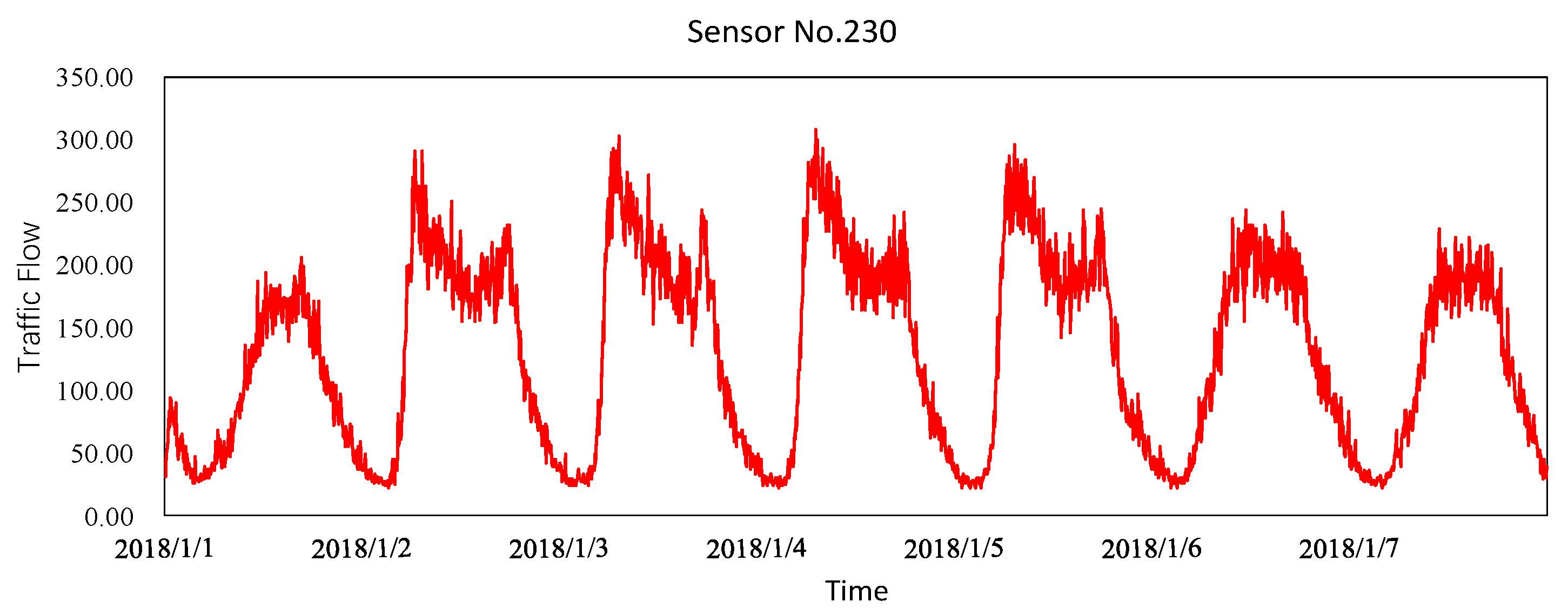
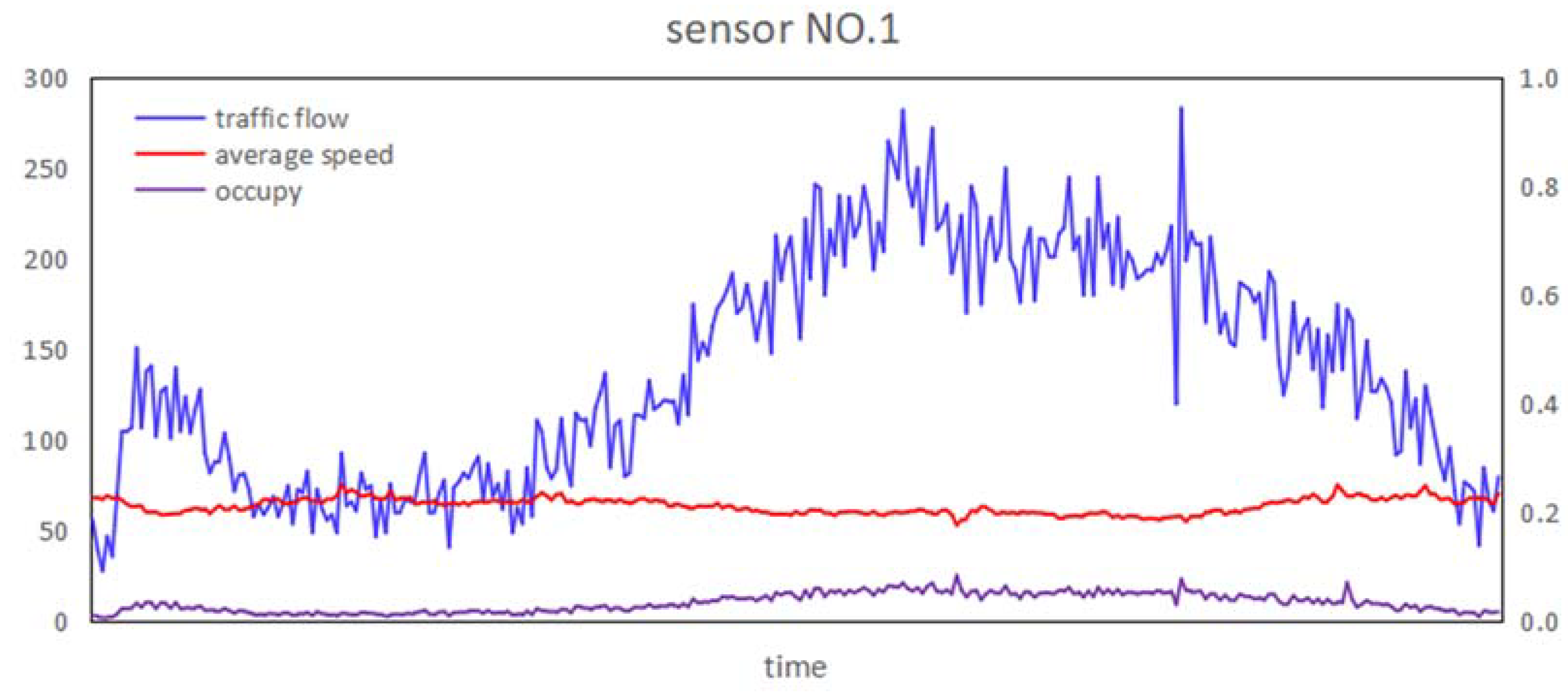
Time dependence: the traffic flow at a given moment is usually correlated with various historical values [6]. One example is that a traffic jam on a road will inevitably affect its flow during commuters’ “rush” hours. As shown in Figure 1, the traffic flow of a road can be predicted based on its own recent flow and periodic flow.

(2)

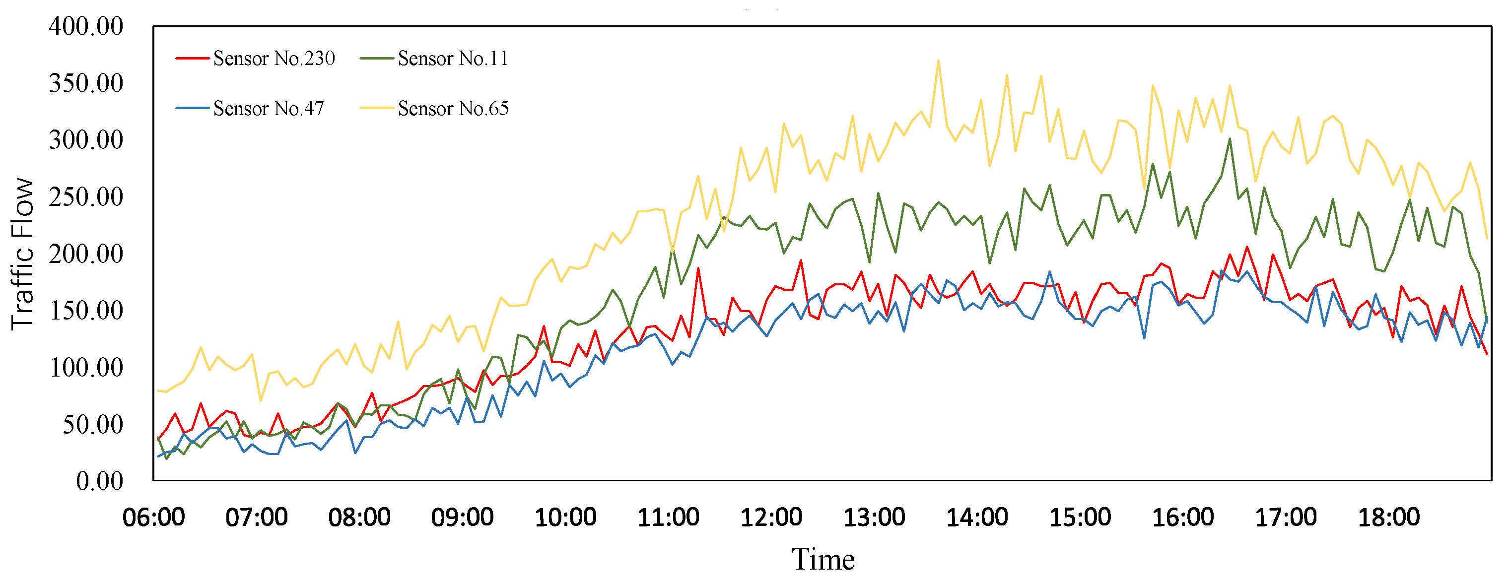
Spatial dependence: the traffic condition of one road is affected by its adjacent roads or even indirectly connected roads. We can see from Figure 2 that the change in traffic flow is dominated by the topological structure of the traffic network. The traffic statuses of adjacent roads influence one another.

Previous studies usually regarded traffic data as a time series and predicted future traffic conditions through regression analysis of time-series data [7,8,9,10]. However, these methods seldom take the interaction between roads into account. The prediction results are rarely accurate as they make inadequate use of spatial structure information relating to the urban road network. To capture spatial features, some researchers [11,12,13] divided cities into regular grids and introduced a convolutional network (CNN) to model spatial dependence. However, the internal connection modes of graphically structured data are usually complex and diverse. As such, a standard convolution for regular grids is clearly not appropriate for learning and expressing the non-Euclidean features of a graph. Aiming to solve the above problems, we propose a novel hybrid prediction model based on deep learning in this study. The main contributions are as follows:

(a)

We study the traffic flow prediction problem under intelligent transportation and propose a novel hybrid deep-learning-based traffic flow prediction model to provide information and decision support for solving road congestion, thus helping the sustainable development of the city;

(b)

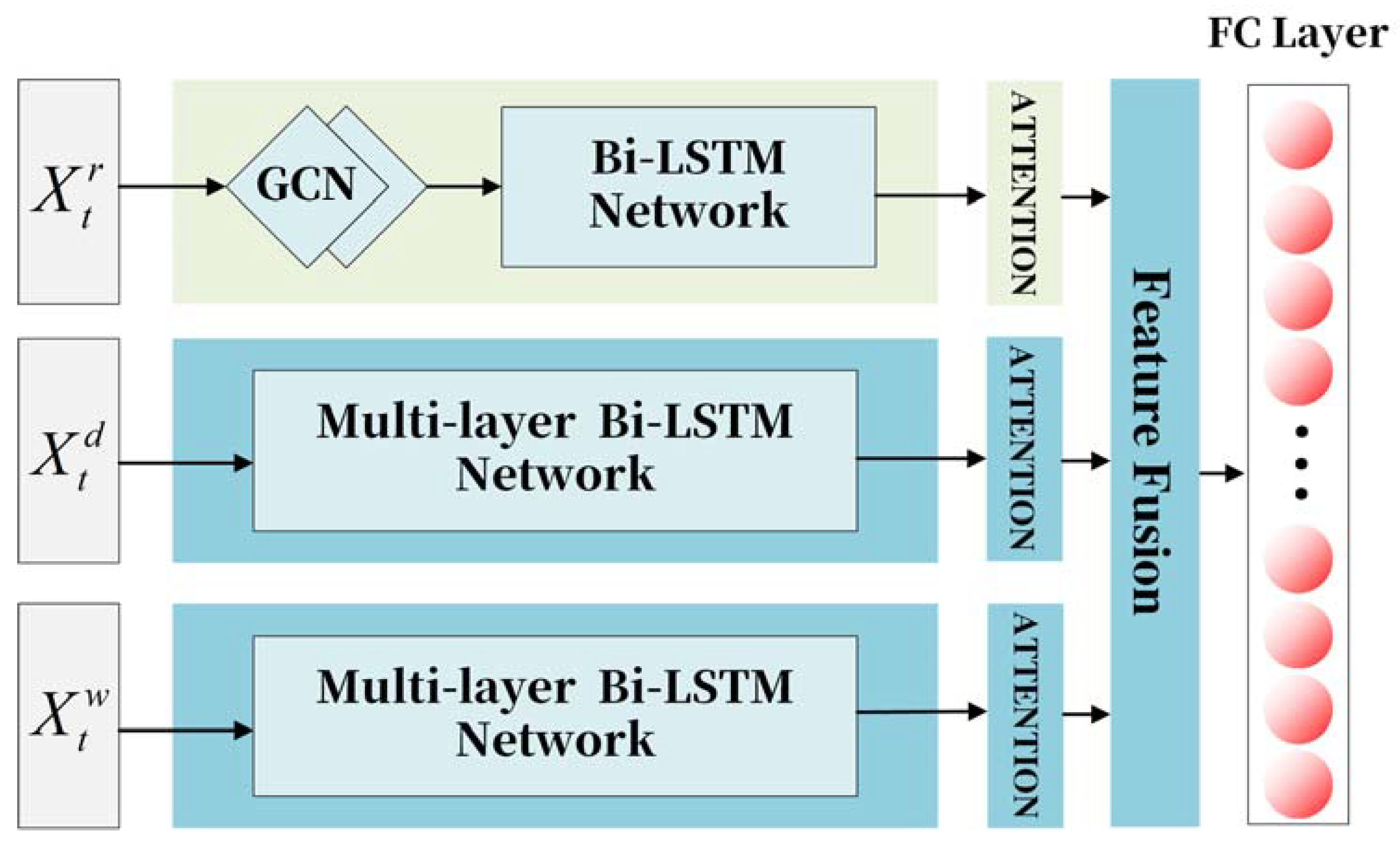
Aiming at the complex situation of traffic in the city, our proposed model uses GCN and Bi-LSTM to model the spatiotemporal dependence and periodicity of traffic data. Moreover, we design an attention layer for each component to make the proposed model focus on the information considered meaningful to the prediction result, sidelining auxiliary information;

(c)

The experimental results on a real-world traffic dataset indicate that our model has better prediction performance than those developed previously.

The rest of this paper is organized as follows. Section 2 introduces the related work. Section 3 outlines the overall framework of the proposed traffic prediction model. In Section 4, we evaluate the effectiveness of the proposed model using a real-world dataset, and we compare the prediction performance to that of other models from the literature. Finally, Section 5 concludes the paper.

2. Related Work

Over the past few decades, researchers have proposed a number of short-term traffic-flow prediction methods. We can roughly divide them into two categories: model-driven and data-driven methods. To work stably, model-driven methods not only require complex system modeling and make unrealistic assumptions but also take a lot of computing power [14]. With the rapid development of intelligent transportation systems and the improvements to traffic data collection and storage technology, a large amount of traffic data has been collected, and many researchers have shifted their attention to data-driven methods.

Data-driven methods rely on the traffic data collected from traffic sensors, such as cameras, induction coils, etc. They deduce the changing trends of the data according to the statistical laws of the data. They commonly build the prediction model based on historical data and gain prediction results by inputting real-time data into the prediction model. Among them, we can roughly divide the models into two categories: parametric and non-parametric models [15].

Usually, the structure of parametric models is predetermined by theoretical assumptions, and the parameters can be calculated using historical data. The widely used parametric approaches for traffic prediction are the time-series model, regression model, the Kalman filter model, etc. Hamed et al. [16] established a time-series model for urban arterial road traffic volume prediction by using ARIMA. To improve the prediction performance, researchers have proposed many variational models of ARIMA such as seasonal ARIMA [9], KARIMA [17] and subset ARIMA [7]. Ni et al. [18] combined wavelet analysis and the ARIMA model to improve the traffic-flow prediction performance. The proposed model firstly used wavelet analysis to decompose the original traffic information into time series with different characteristics and then used ARIMA to model the time series. Instead of taking up classical methods, Ghosh [19] used Bayesian methods to estimate the parameters of SARIMA models that must be considered in modeling. A Kalman filter model is another important method to predict the traffic flow. Okutani [20] first introduced the Kalman filter method to traffic flow prediction. Kumar [21] then proposed a prediction scheme based on the Kalman filtering technique, which requires only limited input data. Xu [22] proposed a real-time road traffic-state prediction method by combining ARIMA and the Kalman filter method.

Most of the traditional parameter models are simple and fast in calculation but their robustness is poor and they are more suitable for road sections with stable traffic conditions. Non-parametric models can automatically learn statistical regularity if there are enough historical data. The commonly used non-parametric models include the K-nearest neighbor model, support vector regression model, machine learning methods and ensemble learning methods. Zhang [23] established a short-term prediction system of urban expressway flow based on the K-nearest neighbor model from three aspects: historical database, search mechanism, algorithm parameters and prediction plan. Tang [24] proposed a traffic flow prediction model that combines a denoising scheme with a support vector machine. The model’s prediction results were better than those of a model without a denoising strategy. Zhang [25] proposed a hybrid prediction model based on SVR, the model used random forest (RF) to select the most informative feature subset and used an enhanced genetic algorithm (GA) with chaotic features to identify the optimal parameters of the prediction model. Dong [26] propose a short-term traffic flow prediction model that combined wavelet decomposition and reconstruction with an extreme gradient boosting (XGBoost) algorithm. Yang [27] presented a short-term traffic prediction model based on Gradient boosting decision trees (GBDT) and verified the performance of the model on an expressway traffic flow dataset.

In recent years, deep learning methods have been widely used in transportation research and have achieved high accuracy and efficiency. Wei [28] proposed a novel traffic-flow prediction method, called AE-LSTM, where the AutoEncoder is used for feature extraction and the LSTM model is used to make predictions. Luo [29] combined k-nearest neighbor (KNN) and a long short-term memory network (LSTM) to predict the future traffic flow, where KNN was used to find the neighboring stations that had a strong correlation with the test station, and LSTM was utilized to model the temporal dependencies of traffic flow. To fully utilize the spatial-temporal dependences of traffic flow, Wu [30] presented a new deep architecture that combined a Convolutional Network and Long Short memory Networks to predict traffic flow at future moments. 1D CNN was used to exploit the spatial dependence, and LSTM was used to capture the short-term dependence and periodicity of traffic flow. Yu [31] proposed a model called STGCN that was constructed with complete convolution structures, and the model used ChebNet and a temporal convolution network to capture spatial and temporal dependencies. Li [32] proposed a DCRNN model, which used a bidirectional random walk to capture spatial dependence on the graph, and encoder-decoder architecture with schedule sampling was used to capture temporal dependence.

3. Methodology

3.1. Problem Formulation

Since the traffic network structure is the same as a graph structure, and the observed value of the detector for each road is a time series, traffic data can be regarded as graphical data with spatial and temporal dimensions. In our work, we define the entire traffic network as an unweighted graph G = (V, E, A). The detectors in the traffic network are treated as nodes in the graph, and V is the graph node set. E is the set of edges, representing the connection between the nodes in the graph. A is the adjacency matrix, which is used to represent the connection relation in the edge set, while $A\in R^{N\times N}$, N is the number of nodes. The corresponding element in the adjacency matrix A is 1 if an edge exists between two nodes, and 0 otherwise. The observed value of the whole graph at time t can be expressed as a graph signal matrix $X^t=\left[X_1^{\mathrm{t}},X_2^{\mathrm{t}},\dots ,X_n^{\mathrm{t}}\right]\in R^{N\times F}$, where F is the number of features.

Therefore, the problem of spatiotemporal traffic prediction can be described as learning a mapping function f to predict the traffic information at the next T moments based on the given road network topology G and historical observed series ($X_{}^{t-T^{\prime }+1},X_{}^{t-T^{\prime }+2},\dots ,X_{}^t$), as shown in Equation (1):

$$\left[X_{}^{t+1},X_{}^{t+2},\dots ,X_{}^{t+T}\right]=f\left(X_{}^{t-T^{\prime }+1},X_{}^{t-T^{\prime }+2},\dots ,X_{}^t\right)$$

(1)

where T is the length of the target series we need to predict, and $T^{\prime }$ is the length of the historical observed series.

3.2. Overview of the Proposed Model

Figure 3 illustrates the overall architecture of our model, consisting of three components: the recent component, daily component and weekly components. The recent component is used to capture the recent dependence of traffic information, and the other two components are used to capture the periodic dependence. As shown in Figure 3, the recent component consists of a two-layer graph convolutional network and bi-directional LSTM (Bi-LSTM), where the graph convolutional operation is utilized to capture the spatial features and Bi-LSTM is used to obtain the temporal features of the traffic data. The daily and weekly components are constructed from the multi-layer Bi-LSTM, where the multi-layer Bi-LSTM is used to capture the periodic characteristics of traffic flow. Afterward, the spatiotemporal feature and periodicity features obtained by the three network components are fused by serial feature fusion through a feature fusion layer. Finally, an output layer (FC layer) is used to transform the outputs of the feature fusion layer into the expected prediction. In addition, we introduce an attention layer to dynamically adjust the importance of the hidden state vector output by Bi-LSTM to the predicted results.

3.3. Graph Convolutional Network for Spatial Dependence Modeling

Obtaining the complex spatial dependence of traffic data is very important for traffic flow prediction. Restricted by the topology of the traffic network, the traffic condition of one road is affected by the surrounding area or even the distant area. Specifically, the traffic flow is not only affected by the historical status of the road but also by the linked roads in space. Some research divided a city into regular grids and introduced a convolutional network to model this spatial dependence. However, while the CNN is more suitable to use for Euclidean space, such as images, but not for networks with complex topological structures, such as transportation networks [33]. To capture spatial associations from non-Euclidian topological graphs, researchers have proposed a new network structure called graph convolutional network (GCN), which can aggregate neighborhood information for each node in graph structure data through convolution.

Given an adjacency matrix A and graph signal matrix $X_G$, GCN can be understood as obtaining new spatial feature representation through aggregation operation of traffic flow information from the central road section and its adjacent road section, which can be expressed as:

$$\mathrm{GCN}\left(H^{\left(l\right)}\right)=H^{\left(l+1\right)}=\sigma \left({\tilde{D}}^{-\frac{1}{2}}\tilde{A}{\tilde{D}}^{-\frac{1}{2}}{H}^{\left(l\right)}{W}^l\right)\in R^{N\times C^{\prime }}$$

(2)

where $\tilde{A}=A+I_N$ is the adjacent matrix with added self-connections, $I_N$ is the identity matrix, $\tilde{D}$ is the degree matrix, ${\tilde{D}}_{ii}={\displaystyle \sum }_j{\tilde{A}}_{ij}$, $H^{\left(l\right)}$ is the output of l layer, $W^l\in R^{C\times C^{\prime }}$ are learnable parameters, C is the number of input features, $C^{\prime }$ is the number of output features and $\sigma$ denotes the activation function (and we used the Rectified Linear Unit (Relu) in our model).

The graph convolution operation is to aggregate the neighbor features to the node itself, where the contribution degree of each neighbor node is negatively correlated with its degree. In other words, the smaller the degree of the neighbor node, the larger its weight will be in the aggregated operation. Yet, this is not a very reasonable way to measure the degree of association between nodes [34]. To capture the correlation between nodes in the graph more reasonably, we add a learnable mask matrix $W_{mask}$ and multiply it by the elements with the adjacent matrix to adjust the aggregation weight, to make the aggregation more reasonable. At the same time, we stack two graph convolution operations to expand the aggregation area:

$$A_{adjust}=W_{mask}⨂\tilde{A}\in R^{N\times N}$$

(3)

The improved graph convolution operation is:

$$\mathrm{GCN}\left(H^{\left(l\right)}\right)=H^{\left(l+1\right)}=\sigma \left(A_{adjust}{H}^{\left(l\right)}{W}^l\right)$$

(4)

In summary, we use a two-layer GCN model to capture the spatial dependence of the traffic flow. After the GCN operation, the time series with spatial features will be entered into the Bi-LSTM to learn temporal features.

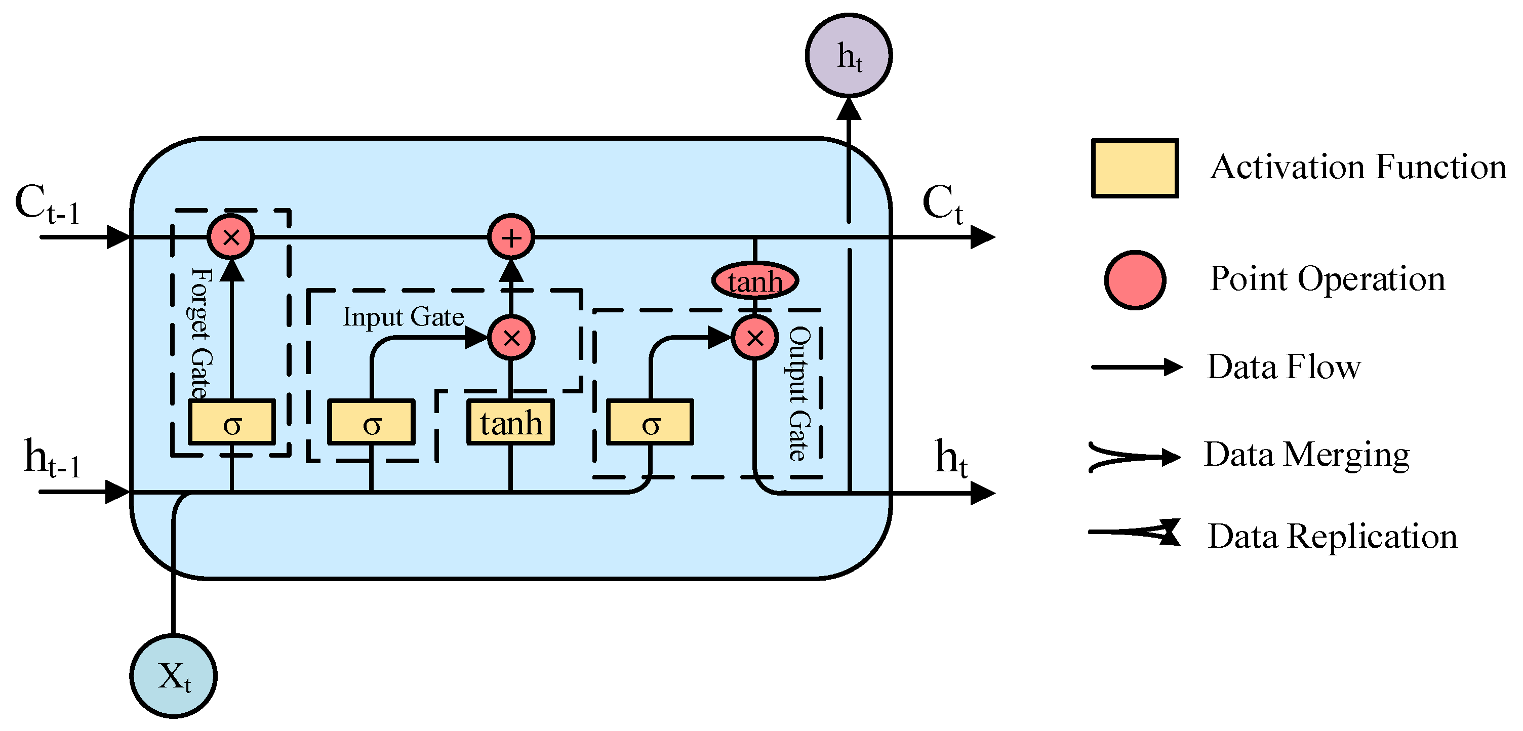
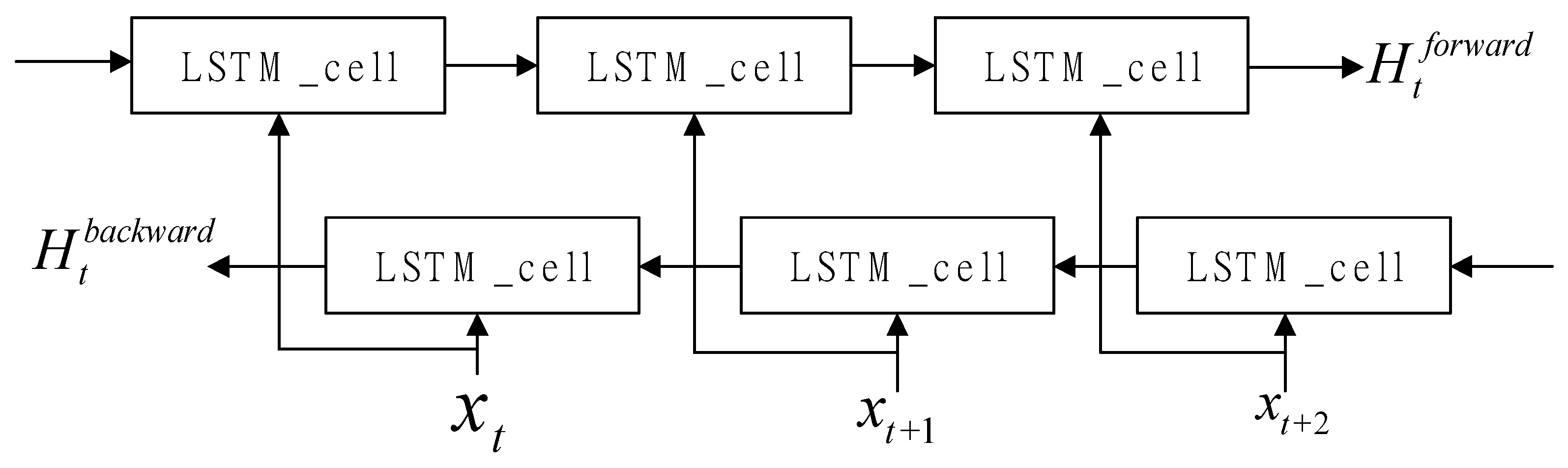
3.4. Bi-Directional LSTM for Temporal Dependence Modeling

Obtaining time dependency is another key problem in traffic prediction. A recurrent neural network (RNN) is commonly used to process data with sequence characteristics. The most representative is the Elman Network, proposed by Elman in 1990, which is the basic version of the widely used traditional RNN. However, the traditional RNN is usually accompanied by the problems of gradient explosion and gradient disappearance when dealing with long time series data. Every LSTM cell adds three control gates-the input gate, forget gate and output gate. and uses three gate mechanisms to control the transmission of information in the network, to realize the long-term memory. The typical structure of the LSTM cell is shown in Figure 4.

In Figure 4, $X_t$ is the input value of the LSTM cell at time $t$, $C_t$ is the state value memory cell at time $t$ and $h_t$ is the output value at time $t$. $\mathsf{\sigma }$ denotes the $sigmoid$ activation function, while $tanh$ means the $tanh$ activation function. The internal calculation process of LSTM can be explained as follows through Equations (5) to (10):

Step 1: calculate the input gate value $i_t$ and the candidate state value $\widetilde{C_t}$ of the cell at time $t$. The specific calculation formulas are as follows:

$$i_t=\delta \left(W_i\ast \left[X_t, h_{t-1}\right]+b_i\right)$$

(5)

$$\widetilde{C_t}=tanh\left(W_c\ast \left[X_t, h_{t-1}\right]+b_c\right)$$

(6)

Step 2: calculate the activation value $f_t$ of the forget gate at time $t$, where the formula is as follows:

$$f_t=\delta \left(W_f\ast \left[X_t, h_{t-1}\right]+b_f\right)$$

(7)

Step 3: calculate the cell state update value $C_t$ at time $t$ and the formula is as follows:

$$C_t=i_t\ast \widetilde{C_t}+f_t\ast C_{t+1}$$

(8)

Step 4: calculate the output value $f_t$ of the output gate at time $t$, where the formula is as follows:

$$o_t=\delta \left(W_o\ast \left[X_t, h_{t-1}\right]+b_o\right)$$

(9)

$$h_t=o_t\mathit{tanh}\left(C_t\right)$$

(10)

where W and b are learnable parameters, representing the weight matrix and bias term in the training process.

As we can see in Figure 5, the bidirectional LSTM network consists of forward and backward LSTMs, one for the forward passage of information and the other for backward passage [35]. The forward LSTM layer is applied to the input sequence, and the reverse form of the input sequence is fed into the backward LSTM layer [36]. Finally, the hidden states of the forward and backward layers are merged into the output. By applying the two unidirectional LSTMs, the shortcoming of the original LSTM that it only uses previous information if it is solved, and the prediction performance is improved [37]. In our work, the Bi-LSTM is adopted to capture the time dependence of traffic flow. Considering the periodicity of traffic information, we also stack multiple Bi-LSTM layers to extract periodic features from historical traffic data.

3.5. Attention Mechanism

An attention mechanism [38] was first used in machine translation to improve the accuracy of machine translation, and now it has become an important tool in the field of artificial neural networks. To put it simply, the attention mechanism focuses on the information that has an important impact on the result and reduces the weight of the information not considered meaningful to the result during feature extraction. Information relating to the traffic flow at different times may be of different levels of importance to the forecast target [35]. For example, when congestion occurs, the traffic state of a distant timestep may have a stronger influence on the predicted target than that of a near timestep.

We adopt an attention mechanism to dynamically adjust the weight of the output of the Bi-LSTM module. The implementation of the attention mechanism can be expressed as:

$${\mu }_{it}=\mathit{tanh}\left(W_w{h}_{it}+b_w\right)$$

(11)

$${\alpha }_{it}=\frac{\exp \left({\mu }_{it}^T{\mu }_w\right)}{{{\displaystyle \sum }}_t\exp \left({\mu }_{it}^T{\mu }_w\right)}$$

(12)

$$s_i={{\displaystyle \sum }}_t{\alpha }_{it}{h}_{it}$$

(13)

where $W_w,$ $b_w,$ ${\mu }_w$ are learnable parameters, ${\alpha }_{it}$ is the attention score and $s_i$ is the output of the attention layer.

3.6. Output Layer

After processing by the attention layer, the spatiotemporal features and periodicity features obtained by the three network components are concentrated into a feature vector through a feature fusion layer. Supposing $X\in R^{N\times C}$ is the input of the output layer, a two-layer fully connected neural network is used to generate one timestep prediction. We use T two-layer fully connected neural networks to generate prediction results for T timesteps in the future. Each timestep prediction result is concentrated to obtain the final prediction. The specific process is as follows:

$$\begin{gathered} {\widehat{y}}^{\left(i\right)}=ReLU\left(X{W}_1^{\left(i\right)}+b_1^{\left(i\right)}\right)·W_2^{\left(i\right)}+b_2^{\left(i\right)}\in R^{N\times 1} \\ \widehat{Y}=\left[{\widehat{y}}^{\left(1\right)},{\widehat{y}}^{\left(2\right)},\dots ,{\widehat{y}}^{\left(T\right)}\right]\in R^{N\times T} \end{gathered}$$

(14)

where ${\widehat{y}}^{\left(i\right)}$ is the prediction in timestep i, $W_1^{\left(i\right)}\in R^{C\times C^{\prime }}$, $b_1^{\left(i\right)}\in R^{C^{\prime }}$, $W_2^{\left(i\right)}\in R^{C^{\prime }\times 1}$ and $b_2^{\left(i\right)}\in R$ are learnable parameters, $C^{\prime }$ is the output dimension of the first fully connected layer.

The loss function of our model is Huber loss [39], and we use $\widehat{Y}$ and Y to denote the predicted and true values. Huber loss is a parametric loss function used in regression problems. It can enhance the robustness of the mean square error (MSE) to outliers. The Huber loss function is shown as follows:

$$\mathrm{L}\left(Y,\widehat{Y}\right)=\left\{\begin{array}{c}\frac{1}{2}{\left(Y-\widehat{Y}\right)}^2 \left|Y-\widehat{Y}\right|\le \delta \\ \delta \left|Y-\widehat{Y}\right|-\frac{1}{2}{\delta }^2 otherwise \end{array}\right.$$

(15)

4. Performance Evaluation

4.1. Dataset Description and Preprocessing

We evaluated the performance of our model on highway traffic dataset PeMSD4 from California. The dataset came from the California Transportation Agency’s Performance Measurement System (PeSM) [40], where traffic sensors in major areas of the Californian highway network collect data at 30-s intervals. To reduce data redundancy, traffic data are aggregated from the original data every 5 min, which means there are 12 points of traffic data each hour [41]. The dataset spanned from 1 January 2018 to 28 February 2018. We used three kinds of traffic measurements—traffic flow, average occupancy and average speed—to predict the traffic flow in the next hour.

Table 1. Dataset information.

Dataset	Nodes	Edges	Length of Dataset	Time Range	Number of Features
PeMS04	307	340	16,992	1 January 2018 to 28 February 2018.	traffic flow average occupancy average speed

shows more detailed information about the dataset, and we randomly visualized the traffic information for one road from the dataset over 24 h (Figure 6).

We intercepted three time-series segments $X^r$, $X^d$ and $X^w$ along the time axis as the inputs for the recent, daily and weekly components, respectively (see Figure 7) [41]. In our work, the three series segments were all 12 in length. $X^r$ was a time series directly adjacent to the prediction period, and $X^d$ and $X^w$ were the same moments from the last day and last week. The dataset was split with a ratio of 6:2:2 into a training set, validation set and test set, respectively, and we used Z-Score standardization to process the data. The calculation formula is as follows:

$$X^{\prime }=\frac{X-mean\left(X\right)}{std\left(X\right)}$$

(16)

where mean(X) is the mean of the historical time series, and std(X) is the standard deviation of the historical time series.

4.2. Index of Performance

In the experiment, the mean absolute error (MAE), mean absolute percentage error (MAPE) and root mean square error (RMSE) were used to evaluate the prediction performance of the model. The three indexes were defined as follows:

$$\mathrm{MAE}=\frac{1}{n}{\displaystyle \sum }_{t=1}^n\left|y_i-\widehat{y_i}\right|$$

(17)

$$\mathrm{MAPE}=\frac{1}{n}{\displaystyle \sum }_{t=1}^n\frac{\left|y_i-\widehat{y_i}\right|}{y_i}\times 100\%$$

(18)

$$\mathrm{RMSE}=\sqrt{\frac{1}{n}{\displaystyle \sum }_{t=1}^n{\left(y_i-\widehat{y_i}\right)}^2}$$

(19)

where $y_i$ denotes the predicted value of the i-th sample, $\widehat{y_i}$ is the true value of the i-th sample and n is the number of samples. The smaller the value of these three performance indexes, the better the prediction performance of the model.

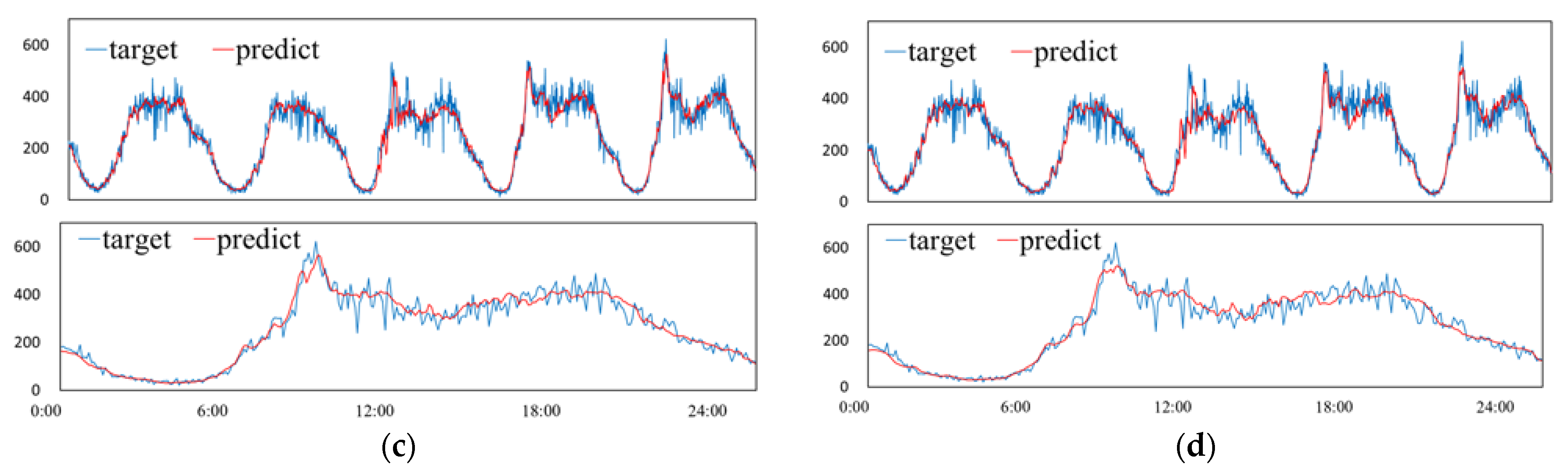
4.3. Experiment Result

The proposed model was implemented using the PyTorch framework [42], and the experiments were conducted on an Nvidia GeForce RTX2080Ti. In the experiment, the model contained two graph convolution operations with 32 filters and 128 hidden units of Bi-LSTM. We stacked two layers of Bi-LSTM to capture the periodic characteristics of traffic data. The optimization algorithm was Adam with a 0.001 initial learning rate since the algorithm could adaptively adjust the learning rate.

We conducted comparative experiments with the following short-term traffic flow prediction methods to evaluate the prediction performance of the proposed model:

(1)

SVR: support vector regression;

(2)

LSTM: long short-term memory networks;

(3)

GCN: graph convolution network;

(4)

STGCN [31]: spatiotemporal graph convolution model, using ChebNet and a temporal convolution network to capture spatial and temporal dependencies;

(5)

ASTGCN [41]: attention-based spatiotemporal graph convolutional networks, using three of the same modules to model periodicity characteristics of traffic data, where each module contains several spatiotemporal blocks designed to capture spatial and temporal dependencies.

The average results of the traffic flow prediction performance for the next hour for different algorithms are shown in

Table 2. Overall prediction performance of different methods for the PeMSD4 dataset.

Model	Dataset	PeMS04
	Metrics	MAE	MAPE (%)	RMSE
SVR		28.96	19.23	45.21
LSTM		27.54	18.96	42.54
GCN		25.06	17.04	38.67
STGCN		22.83	14.62	35.79
ASTGCN		21.94	14.23	32.76
Our Model		20.00	13.95	32.41

. From the table, we can see that our model achieved the best performance for all evaluation indexes. All models considering the spatiotemporal characteristics of traffic data achieved better results.

The SVR and LSTM only consider temporal correlations and cannot capture spatial dependency. However, a change in traffic flow is restricted by the topology of a traffic network, and the traffic status of each road is not independent. Therefore, the prediction results for those approaches were the worst. The GCN model considers spatial correlations but cannot capture the temporal dependency. As we all know, traffic exhibits temporal correlations with adjacent times. The STSGCN and ASTGCN take spatial and temporal dependencies into account. The STGCN model is constructed with complete convolution structures, which can achieve a faster training speed with fewer parameters. It uses a graph convolution operation and gated CNNs to model the spatial and temporal dependencies of the traffic data. The ASTGCN uses three of the same modules to model periodicity characteristics of traffic data, with each module containing several spatiotemporal blocks designed to capture spatial and temporal dependencies. The prediction result of ASTGCN is obtained by fusing the outputs of the three modules., From Table 2, we can see that our model achieved better results than the other models. The MAE, MAPE and RMSE are reduced by 1.94, 0.28 and 0.35 compared with the best base model ASTGCN. By considering the spatiotemporal dependencies and periodicity characteristics of traffic data, our model could reduce the prediction errors.

Figure 8 shows the overall performance of our model. From Figure 8, we can see that with an increase in the prediction timestep, the difficulty of prediction increased gradually, and the prediction error of the model became larger. To better show the prediction results of our proposed model, we randomly choose one road on the dataset and visualize the prediction results. Figure 9 shows the visualization results for prediction horizons of 5 min, 15 min, 30 min and 60 min. We can see the prediction error between the predicted value and the ground truth for one road segment in a given period in Figure 9. We can find that the variation trend for traffic flow predicted by our model was generally consistent with the variation trend to the real values. However, the curve of the predicted value of the model is smoother than that of the real value.

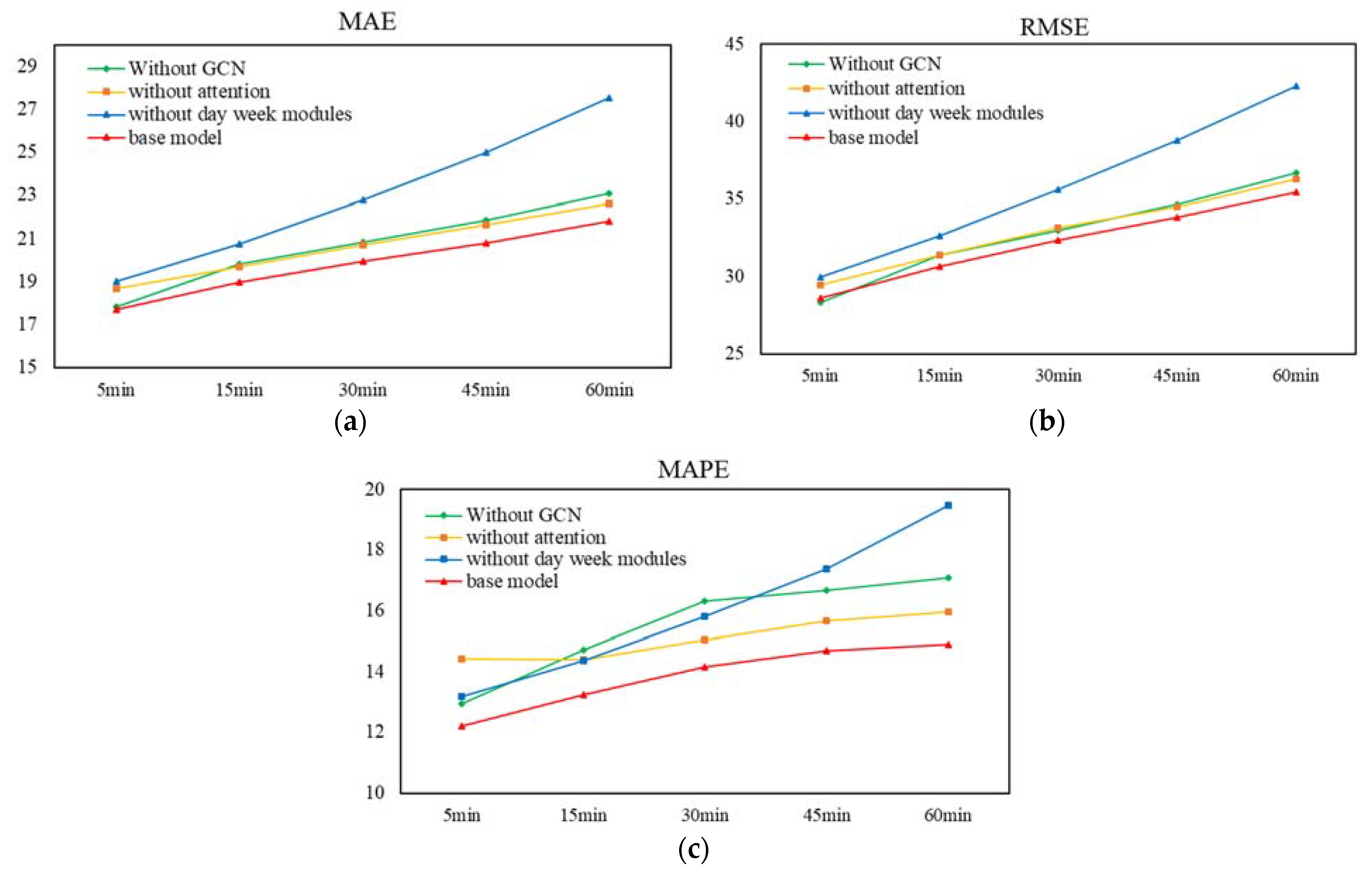
4.4. Component Analysis

In this section, we present three variants of our model designed to further investigate the effects of different modules. All the variants have the same training parameters. The differences between the models are as follows:

(1)

Base model: we do not remove any modules from the proposed model;

(2)

Without GCN: we remove the graph convolution operation to evaluate the ability to extract spatial features with the proposed model;

(3)

Without attention: this model is made without any attention mechanism;

(4)

Without day or week modules: we remove the daily and weekly components to evaluate the ability to extract periodicity features with the proposed model.

We first evaluate the ability to extract spatial features with the proposed model. Figure 10 shows the performance of the variant model without GCN. We can see that the error between the predicted value and the ground truth is larger than with our model. This is because the change in traffic flow is restricted by the topology of the traffic network; the traffic always shows a spatial dependency, but the variant model cannot capture this spatial dependency.

Next, we evaluate the prediction performance of the proposed attention module. The attention mechanism can help the model focus on the information that has an important impact on the result during feature extraction. As we can see from Figure 10, the MAE, MAPE and RMSE have increased without the attention mechanism. Evidently, the attention module can help the model to get a better prediction result.

Furthermore, we evaluate the ability of the proposed model to extract periodicity features. We remove the day and week modules from our model and only take ${\mathrm{X}}_{}^r$ as the model input. Traffic flow has a strong periodic tendency, and in the experiment without the two modules, our model had a significant performance decline, as shown in Figure 10. Evidently, periodic features are needed to get a good prediction result in time-series forecasting.

5. Conclusions

Accurate short-term traffic flow prediction will bring great convenience to people’s travel, not only supporting effective travel route planning but also reducing accident rates. Such prediction is the key to constructing intelligent transportation, which will play an important role in the sustainable development of cities. In this paper, the short-term traffic flow prediction of an intelligent transportation system was studied. A novel hybrid deep learning prediction model was designed to deal with the complex, nonlinear characteristics of traffic flow. The proposed model uses a graph convolutional neural network to capture the spatial features of traffic flow and uses bidirectional LSTM to model the time dependence. A multi-layer Bi-LSTM module was designed to extract periodic features. Experimental results when using the PeMS04 dataset showed that the proposed model had a better prediction performance compared to those of past methods. However, many factors affect traffic flow in reality [43], such as weather conditions, events, etc. In the future, more factors should be included in such experiments, to gain better traffic-flow prediction results.

References

1. Su, X.; Zheng, C.; Yang, Y.; Yang, Y.; Zhao, W.; Yu, Y. Spatial Structure and Development Patterns of Urban Traffic Flow Network in Less Developed Areas: A Sustainable Development Perspective. Sustainability 2022, 14, 8095. [Google Scholar] [CrossRef]
2. Wang, Z.; Chu, R.; Zhang, M.; Wang, X.; Luan, S. An Improved Hybrid Highway Traffic Flow Prediction Model Based on Machine Learning. Sustainability 2020, 12, 8298. [Google Scholar] [CrossRef]
3. Khan, N.U.; Shah, M.A.; Maple, C.; Ahmed, E.; Asghar, N. Traffic Flow Prediction: An Intelligent Scheme for Forecasting Traffic Flow Using Air Pollution Data in Smart Cities with Bagging Ensemble. Sustainability 2022, 14, 4164. [Google Scholar] [CrossRef]
4. Sumalee, A.; Ho, H.W. Smarter and more connected: Future intelligent transportation system. Iatss Res. 2018, 42, 67–71. [Google Scholar] [CrossRef]
5. Xu, X.; Huang, Q.; Zhu, H.; Sharma, S.; Zhang, X.; Qi, L.; Bhuiyan, M.Z.A. Secure service offloading for Internet of vehicles in SDN-enabled mobile edge computing. IEEE Trans. Intell. Transp. Syst. 2020, 22, 3720–3729. [Google Scholar] [CrossRef]
6. Ye, J.; Zhao, J.; Ye, K.; Xu, C. How to build a graph-based deep learning architecture in traffic domain: A survey. IEEE Trans. Intell. Transp. Syst. 2020, 23, 3904–3924. [Google Scholar] [CrossRef]
7. Lee, S.; Fambro, D.B. Application of subset autoregressive integrated moving average model for short-term freeway traffic volume forecasting. Transp. Res. Rec. 1999, 1678, 179–188. [Google Scholar] [CrossRef]
8. Fu, R.; Zhang, Z.; Li, L. Using LSTM and GRU neural network methods for traffic flow prediction. In Proceedings of the 2016 31st Youth Academic Annual Conference of Chinese Association of Automation (YAC) IEEE, Wuhan, China, 11–13 November 2016; pp. 324–328. [Google Scholar]
9. Williams, B.M.; Hoel, L.A. Modeling and forecasting vehicular traffic flow as a seasonal ARIMA process: Theoretical basis and empirical results. J. Transp. Eng. 2003, 129, 664–672. [Google Scholar] [CrossRef]
10. Hong, W.-C.; Dong, Y.; Zheng, F.; Wei, S.Y. Hybrid evolutionary algorithms in a SVR traffic flow forecasting model. Appl. Math. Comput. 2011, 217, 6733–6747. [Google Scholar] [CrossRef]
11. Ranjan, N.; Bhandari, S.; Zhao, H.P.; Kim, H.; Khan, P. City-wide traffic congestion prediction based on CNN, LSTM and transpose CNN. IEEE Access 2020, 8, 81606–81620. [Google Scholar] [CrossRef]
12. Cao, M.; Li, V.O.K.; Chan, V.W.S. A CNN-LSTM model for traffic speed prediction. In Proceedings of the 2020 IEEE 91st Vehicular Technology Conference (VTC2020-Spring), Antwerp, Belgium, 25–28 May 2020; IEEE: Antwerp, Belgium, 2020; pp. 1–5. [Google Scholar]
13. Zhang, J.; Zheng, Y.; Qi, D. Deep spatio-temporal residual networks for citywide crowd flows prediction. In Proceedings of the Thirty-First AAAI Conference on Artificial Intelligence, San Francisco, CA, USA, 4–9 February 2017. [Google Scholar]
14. Vlahogianni, E.I. Computational intelligence and optimization for transportation big data: Challenges and opportunities. Eng. Appl. Sci. Optim. 2015, 38, 107–128. [Google Scholar]
15. Koesdwiady, A.; Soua, R.; Karray, F. Improving traffic flow prediction with weather information in connected cars: A deep learning approach. IEEE Trans. Veh. Technol. 2016, 65, 9508–9517. [Google Scholar] [CrossRef]
16. Hamed, M.M.; Al-Masaeid, H.R.; Said, Z.M.B. Short-term prediction of traffic volume in urban arterials. J. Transp. Eng. 1995, 121, 249–254. [Google Scholar] [CrossRef]
17. Van Der Voort, M.; Dougherty, M.; Watson, S. Combining Kohonen maps with ARIMA time series models to forecast traffic flow. Transp. Res. Part C Emerg. Technol. 1996, 4, 307–318. [Google Scholar] [CrossRef]
18. Lihua, N.; Xiaorong, C.; Qian, H. ARIMA model for traffic flow prediction based on wavelet analysis. In Proceedings of the 2nd International Conference on Information Science and Engineering, Hangzhou, China, 4–6 December 2010; IEEE: Hangzhou, China, 2010; pp. 1028–1031. [Google Scholar]
19. Ghosh, B.; Basu, B.; O’Mahony, M. Bayesian time-series model for short-term traffic flow forecasting. J. Transp. Eng. 2007, 133, 180–189. [Google Scholar] [CrossRef]
20. Okutani, I.; Stephanedes, Y.J. Dynamic prediction of traffic volume through Kalman filtering theory. Transp. Res. Part B Methodol. 1984, 18, 1–11. [Google Scholar] [CrossRef]
21. Kumar, S.V. Traffic flow prediction using Kalman filtering technique. Procedia Eng. 2017, 187, 582–587. [Google Scholar] [CrossRef]
22. Xu, D.; Wang, Y.; Jia, L.; Qin, Y.; Dong, H. Real-time road traffic state prediction based on ARIMA and Kalman filter. Front. Inf. Technol. Electron. Eng. 2017, 18, 287–302. [Google Scholar] [CrossRef]
23. Zhang, L.; Liu, Q.; Yang, W.; Wei, N.; Dong, D. An improved k-nearest neighbor model for short-term traffic flow prediction. Procedia-Soc. Behav. Sci. 2013, 96, 653–662. [Google Scholar] [CrossRef]
24. Tang, J.; Chen, X.; Hu, Z.; Zong, F.; Han, C.; Li, L. Traffic flow prediction based on combination of support vector machine and data denoising schemes. Phys. A Stat. Mech. Its Appl. 2019, 534, 120642. [Google Scholar] [CrossRef]
25. Zhang, L.; Alharbe, N.R.; Luo, G.; Yao, Z.; Li, Y. A hybrid forecasting framework based on support vector regression with a modified genetic algorithm and a random forest for traffic flow prediction. Tsinghua Sci. Technol. 2018, 23, 479–492. [Google Scholar] [CrossRef]
26. Dong, X.; Lei, T.; Jin, S.; Hou, Z. Short-term traffic flow prediction based on XGBoost. In Proceedings of the 2018 IEEE 7th Data Driven Control and Learning Systems Conference (DDCLS), Enshi, China, 25–27 May 2018; IEEE: Enshi, China, 2018; pp. 854–859. [Google Scholar]
27. Yang, S.; Wu, J.; Du, Y.; He, Y.; Chen, X. Ensemble learning for short-term traffic prediction based on gradient boosting machine. J. Sens. 2017, 2017, 7074143. [Google Scholar] [CrossRef]
28. Wei, W.; Wu, H.; Ma, H. An autoencoder and LSTM-based traffic flow prediction method. Sensors 2019, 19, 2946. [Google Scholar] [CrossRef] [PubMed]
29. Luo, X.; Li, D.; Yang, Y.; Zhang, S. Spatiotemporal traffic flow prediction with KNN and LSTM. J. Adv. Transp. 2019, 2019, 4145353. [Google Scholar] [CrossRef]
30. Wu, Y.; Tan, H. Short-term traffic flow forecasting with spatial-temporal correlation in a hybrid deep learning framework. arXiv 2016, arXiv:1612.01022. [Google Scholar]
31. Yu, B.; Yin, H.; Zhu, Z. Spatio-temporal graph convolutional networks: A deep learning framework for traffic forecasting. arXiv 2017, arXiv:1709.04875. [Google Scholar]
32. Li, Y.; Yu, R.; Shahabi, C.; Liu, Y. Diffusion convolutional recurrent neural network: Data-driven traffic forecasting. arXiv 2017, arXiv:1707.01926. [Google Scholar]
33. Zhao, L.; Song, Y.; Zhang, C.; Liu, Y.; Wang, P.; Lin, T.; Deng, M.; Li, H. T-gcn: A temporal graph convolutional network for traffic prediction. IEEE Trans. Intell. Transp. Syst. 2019, 21, 3848–3858. [Google Scholar] [CrossRef]
34. Song, C.; Lin, Y.; Guo, S.; Wan, H. Spatial-temporal synchronous graph convolutional networks: A new framework for spatial-temporal network data forecasting. In Proceedings of the AAAI Conference on Artificial Intelligence, New York, NY, USA, 7–12 February 2020; Volume 34, pp. 914–921. [Google Scholar]
35. Zheng, H.; Lin, F.; Feng, X.; Chen, Y. A hybrid deep learning model with attention-based conv-LSTM networks for short-term traffic flow prediction. IEEE Trans. Intell. Transp. Syst. 2020, 22, 6910–6920. [Google Scholar] [CrossRef]
36. Siami-Namini, S.; Tavakoli, N.; Namin, A.S. The performance of LSTM and BiLSTM in forecasting time series. In Proceedings of the 2019 IEEE International Conference on Big Data (Big Data), IEEE, Los Angeles, CA, USA, 9–12 December 2019; pp. 3285–3292. [Google Scholar]
37. Baldi, P.; Brunak, S.; Frasconi, P.; Soda, G.; Pollastri, G. Exploiting the past and the future in protein secondary structure prediction. Bioinformatics 1999, 15, 937–946. [Google Scholar] [CrossRef]
38. Vaswani, A.; Shazeer, N.; Parmar, N.; Uszkoreit, J.; Jones, L.; Gomez, A.N.; Kaiser, Ł.; Polosukhin, I. Attention is all you need. In Proceedings of the Advances in Neural Information Processing Systems 30: Annual Conference on Neural Information Processing Systems, Long Beach, CA, USA, 4–9 December 2017; pp. 5998–6008. [Google Scholar]
39. Huber, P.J. Robust estimation of a location parameter. In Breakthroughs in Statistics; Springer: New York, NY, USA, 1992; pp. 492–518. [Google Scholar]
40. Chen, C.; Petty, K.; Skabardonis, A.; Varaiya, P.; Jia, Z. Freeway performance measurement system: Mining loop detector data. Transp. Res. Rec. 2001, 1748, 96–102. [Google Scholar] [CrossRef]
41. Guo, S.; Lin, Y.; Feng, N.; Song, C.; Wan, H. Attention based spatial-temporal graph convolutional networks for traffic flow forecasting. In Proceedings of the AAAI Conference on Artificial Intelligence, Honolulu, HI, USA, 27 January–1 February 2019; Volume 33, pp. 922–929. [Google Scholar]
42. Paszke, A.; Gross, S.; Massa, F.; Lerer, A.; Bradbury, J.; Chanan, G.; Killeen, T.; Lin, Z.; Gimelshein, N.; Antiga, L.; et al. Pytorch: An imperative style, high-performance deep learning library. In Advances in Neural Information Processing Systems; Curran Associates, Inc.: Red Hook, NY, USA, 2019; Volume 32, pp. 8024–8035. [Google Scholar]
43. Tian, C.; Chan, W.K. Spatial-temporal attention wavenet: A deep learning framework for traffic prediction considering spatial-temporal dependencies. IET Intell. Transp. Syst. 2021, 15, 549–561. [Google Scholar] [CrossRef]
Figure 1. Traffic flow for one road over a set period.
Sustainability 14 10039 g001
Figure 2. Traffic flows of four adjacent roads over a set period.
Sustainability 14 10039 g002
Figure 3. Architecture of the proposed prediction model.
Sustainability 14 10039 g003
Figure 4. LSTM Memory Cell Unit Structure.
Sustainability 14 10039 g004
Figure 5. Structure of Bi-LSTM networks.
Sustainability 14 10039 g005
Figure 6. Visualization of the traffic information for one road within 24 h.
Sustainability 14 10039 g006
Figure 7. Example of the input time series segment.
Sustainability 14 10039 g007
Figure 8. Prediction performance of our model.
Sustainability 14 10039 g008
Figure 9. The visualization of prediction results. (a) prediction horizon of 5 min. (b) prediction horizon of 15 min. (c) prediction horizon of 30 min. (d) prediction horizon of 60 min.
Sustainability 14 10039 g009aSustainability 14 10039 g009b
Figure 10. Performance of different variants of proposed model. (a) comparison of MAE. (b) comparison of RMSE. (c) comparison of MAPE.
Sustainability 14 10039 g010