Minimum Safety Factor Evaluation of Slopes Using Hybrid Chaotic Sand Cat and Pattern Search Approach

Abstract

This study developed an efficient evolutionary hybrid optimization technique based on chaotic sand cat optimization (CSCO) and pattern search (PS) for the evaluation of the minimum safety factor of earth slopes under static and earthquake loading conditions. To improve the sand cat optimization approach’s exploration ability, while also avoiding premature convergence, the chaotic sequence was implemented. The proposed hybrid algorithm (CSCPS) benefits from the effective global search ability of the chaotic sand cat optimization, as well as the powerful local search capability of the pattern search method. The suggested CSCPS algorithm’s efficiency was confirmed by using mathematical test functions, and its findings were compared with standard SCO, as well as some efficient optimization techniques. Then the CSCPS was applied for the calculation of the minimum safety factors of the earth slope exposed to both static and seismic loads, and the objective function was modeled based on the Morgenstern–Price limit equilibrium method, along with the pseudo-static approach. The CSCPS’s efficacy for the evaluation of the minimum safety factor of slopes was investigated by considering two case studies from the literature. The numerical experiments demonstrate that the new algorithm could generate better optimal solutions via calculating lower values of safety factors by up to 10% compared with some other methods in the literature. Furthermore, the results show that, through an increase in the acceleration coefficient to 0.1 and 0.2, the factor of safety decreased by 19% and 32%, respectively.

1. Introduction

Slope failure is a common cause of fatalities and property damage. As a result, geotechnical engineers must determine the minimal slope safety factor and find the critical slip surface [1,2]. In general, slope safety testing is performed while the slope is subjected to static loads. In an earthquake-prone area, the stability assessment of a slope exposed to dynamic loads should be thoroughly investigated. Various methods, such as finite element analysis, limit equilibrium, limit analysis method, probabilistic analysis methods, and others, have been developed for this analysis. However, limit equilibrium is the most widely used analytical approach for geotechnical studies [3]. These methods function by slicing the entire slide slope mass into a fixed number of vertical slices and evaluating the probable slip surfaces and their associated safety factors in terms of various active forces. In the limit equilibrium approach, the slope’s stability is determined by the lowest factor of safety (FOS) connected to the major failure surface. For seismic slope safety analysis, the pseudo-static technique is the most popular process. This concept has been used in limit equilibrium methods, in which an equivalent static force (F_h) can be used to predict the outcome of an earthquake. The horizontal acceleration coefficient (K_h) and projected sliding mass weight determine the magnitude of this force [4].

In the analysis of earth slopes, the main slip surface correlated to the lowest factor of safety needs to be discovered among viable trial slip surfaces. This issue may be solved by using either traditional deterministic or newer metaheuristic optimization techniques. Slope-stability evaluation is essentially a nondeterministic polynomial-time complete (NPC) problem and is one of the most difficult types of problems due to variation in soil properties, ground conditions, and external forces [5]. When the search space comprises numerous local minima and the computational complexity environment is high, traditional deterministic techniques fail to provide a feasible solution. On the other hand, metaheuristic algorithms have simple notions and structures, derivation-free methods, and are successful for both continuous and discrete functions. Accordingly, several research efforts have been attempted to implement various metaheuristic strategies for slope stability estimation based on these benefits. Some of these studies include implementation of a genetic algorithm [6,7], simulated annealing and harmony search [8], imperialistic competitive algorithm [9], biogeography-based optimization [10], and particle swarm optimization [11,12].

Despite the fact that metaheuristic methods can produce acceptable results, no algorithm outperforms another in solving all optimization problems. Furthermore, the objective function in most geotechnical engineering optimization problems, such as slope stability, foundation, and retaining structures optimization, has a lot of design variables and is discontinuous. Due to this, numerous investigations have been undertaken in order to improve the effectiveness and robustness of the existing metaheuristics. These include modified particle swarm optimization [13,14,15], modified harmony search algorithm [16], modified gravitational search algorithm [17], modified sine cosine algorithm [18], improved salp swarm algorithm [19], modified ant colony optimization [20], modified teaching-learning-based optimization [21], improved tunicate swarm algorithm [22], and modified wild horse optimization [23]. According to the effectiveness of the metaheuristics and their modified versions, these methods have been widely used to solve several geotechnical engineering problems, as presented in Table 1. In addition, a comprehensive review of slope stability analysis methods can be found in References [24,25,26,27].

Table 1. Application of metaheuristic algorithms for geotechnical engineering problems.

Author, Year	Reference	Optimization Method	Application
Goh, 2000	[28]	Genetic algorithm	Locate the critical circular slip surface in slope stability analysis
Zolfaghari, Heath, and McCombie, 2005	[6]	Genetic algorithm	In slope stability, look for critical non-circular failure surfaces.
Cheng et al., 2007	[29]	Particle swarm optimization	Two-dimensional slope stability analysis
Cheng et al., 2008	[16]	Improved harmony search algorithm	Slope stability analysis
Chan, Zhang, and Ng, 2009	[30]	Hybrid genetic algorithms	Optimization of pile groups
Kahatadeniya, Nanakorn, and Neaupane, 2009	[31]	Ant colony optimization	Determination of the critical failure surface of earth slope
Khajehzadeh et al., 2011	[32]	Modified particle swarm optimization	Optimum design of spread footing and retaining wall
Camp and Akin, 2012	[33]	Big bang–big crunch optimization	Optimum design of retaining wall
Camp and Assadollahi, 2013	[34]	Hybrid big bang–big crunch algorithm	Optimizing the cost and CO2 of concrete footings
Khajehzadeh, Taha, and Eslami, 2013	[35]	hybrid firefly algorithm	Minimize of total cost and CO2 emissions of the foundation subjected to geotechnical and structural requirements.
Kang, Li, and Ma, 2013	[36]	Artificial bee colony algorithm	In slope stability, finding the critical slip surface
Khajehzadeh, Taha, and Eslami, 2014	[37]	Adaptive gravitational search algorithm	Multi-objective optimization of foundation
Kashani, Gandomi, and Mousavi, 2016	[9]	Imperialistic competitive algorithm	Locating the critical slip surface of earth slope
Gordan et al., 2016	[38]	Particle swarm optimization and neural network	Prediction of seismic slope stability
Gandomi and Kashani, 2017	[39]	Accelerated particle swarm optimization, firefly algorithm, levy-flight krill herd, whale optimization algorithm, ant lion optimizer, grey wolf optimizer, moth–flame optimization algorithm, and teaching-learning-based optimization algorithm	Construction cost minimization of shallow foundation
Aydogdu, 2017	[40]	Biogeography-based optimization algorithm	Cost optimization of retaining wall
Gandomi et al., 2017	[10]	Genetic algorithm, differential evolution, evolutionary strategy, and biogeography-based optimization	Slope stability analysis
Mahdiyar et al., 2017	[41]	Monte Carlo simulation technique	Safety assessment of slope
Gandomi, Kashani, and Zeighami, 2017	[42]	Interior search algorithm	Retaining wall optimization
Chen et al., 2019	[43]	Hybrid imperialist competitive algorithm and artificial neural network	Prediction of safety factor values of retaining walls
Koopialipoor et al., 2019	[44]	Imperialist competitive algorithm, genetic algorithm, particle swarm optimization, and artificial bee colony combined with artificial neural network	Predict the slope safety exposed to static and dynamic conditions
Yang et al., 2019	[45]	Neural network system	Design retaining wall structures based on smart and optimal systems
Xu et al., 2019	[46]	Hybrid artificial neural network and ant colony optimization	Dynamic conditions of retaining wall structures
Himanshu and Burman, 2019	[11]	Particle swarm optimization	Determination of critical failure surface considering seepage and seismic loading
Kalemci et al., 2020	[47]	Grey wolf optimization algorithm	Optimization of retaining walls
Kaveh, Hamedani, and Bakhshpoori, 2020	[48]	Eleven meta-heuristic algorithms	Optimal design of cantilever retaining walls
Kashani et al., 2020	[49]	Differential algorithm, evolution strategy, and biogeography-based optimization algorithm	Optimum design of shallow foundation
Wang et al., 2020	[50]	Extreme gradient boosting method	Evaluating the earth dam slopefailure probability.
Moayedi et al., 2021	[51]	Harris hawks’ optimization	Predicting the factor of safety in the presence of rigid foundations
Sharma, Saha, and Lohar, 2021	[52]	Hybrid butterfly and symbiosis organism search algorithm	Optimization of retaining wall
Kaveh and Seddighian, 2021	[53]	Black hole mechanics optimization, firefly algorithm, evolution strategy, sine cosine algorithm	Slope critical surfaces optimization with seepage and seismic effects
Temur, 2021	[54]	Teaching-learning based optimization	Optimization of retaining wall
Li and Wu, 2021	[55]	Improved salp swarm algorithm	Locating critical slip surface of slopes
Arabali et al., 2022	[56]	Adaptive tunicate swarm algorithm	Optimization of construction cost and CO2 emissions of shallow foundation
Khajehzadeh, Keawsawasvong, and Nehdi, 2022	[57]	Artificial neural networks combined with rat swarm optimization	Prediction of the ultimate bearing capacity of shallow foundations and their optimum design
Khajehzadeh, Kalhor, et al., 2022	[58]	Adaptive sperm swarm optimization	Optimum design of retaining structures under seismic load
Kashani et al., 2022	[59]	Multi-objective particle swarm optimization, multi-objective multi-verse optimization, and Pareto envelope-based selection algorithm	Multi-objective optimization of mechanically stabilized earth retaining wall

Proposing novel optimization strategies to solve real-world issues, as evidenced by the literature analysis, is highly desirable. The sand cat optimization (SCO) approach is a newly created bioinspired meta-heuristic optimization strategy inspired by the search and hunting behavior of the sand cat. It was first suggested by Seyyedabbasi and Kiani [60]. The low-frequency noise detection behavior of sand cats to find prey was the subject of the sand cat algorithm development [60]. The SCO outperforms other competitive methods in terms of identifying optimal solutions and is well suited to real-world optimization challenges. The chaotic sand cat optimization (CSCO) is an improved variant of the original SCO introduced in this study that uses chaotic sequences to enhance the algorithm’s searching and exploration capabilities.

A balance of exploitation and exploration must be maintained throughout the search operation to achieve an optimum performance when utilizing any optimization technique. Exploration is the process of investigating the search space as widely as possible and visiting entirely new points in it. Conversely, exploitation is the process of refining those points and the local search ability around the promising areas gained in the exploration phase. Because CSCO is a global search strategy, it searches a large area and may not provide the best result if used alone. Search engine techniques, such as pattern search (PS), take advantage of the local but can perform a comprehensive search [61]. There is scope for hybridizing these methods due to their separate capabilities.

Consequently, the following can be used to summarize the main contributions of this work:

• An efficient hybrid metaheuristic approach based on chaotic sand cat and pattern search techniques, known as CSCPS, was developed.
• The performance of CSCPS for numerical function optimization was assessed on thirteen common benchmarking functions, and the results were compared with existing commonly used optimization algorithms.
• To demonstrate the efficiency of the proposed technique in solving real-world problems, the new method was used to determine the minimum factor of safety of earth slopes.
• The objective function of a slope stability problem was modeled by using the Morgenstern–Price limit equilibrium approach for the slip surface’s overall shape.
• The efficiency of the proposed CSCPS for slope stability assessment was investigated by using two benchmark problems based on the literature, and the obtained results were compared with those evaluated previously by the other techniques.

2. Safety Factor Formulation

Geotechnical engineering includes the seismic performance of slopes, particularly in earthquake areas. To assess the constancy of a slope, many traditional approaches are used, such as finite elements, strength reduction, and the limit equilibrium [3]; the limit equilibrium is the most widely used analytical method for geotechnical problems, and it employs Mohr’s coulomb criteria to assess the factor of safety (FOS). Several procedures of analysis derived from the limit equilibrium technique are available, and Duncan [62] has thoroughly reviewed and summarized them. The simple or basic methods, such as the ordinary method of slices and the Bishop method, are relevant to a particular sliding surface shape, whereas the rigorous methodologies, such as the Spencer and Morgenstern–Price approaches, are acceptable to any failure surface shape. The complexity of determining the precise behavior of the soil slope increases when earthquake loads are applied. Consequently, an effective pseudo-static process may be used to assess the reliability of the earth’s steep hills exposed to earthquake stresses. The Morgenstern–Price method of slices and the pseudo-static approach were implemented for seismological slope safety assessment in this study.

Morgenstern and Price [63] established a holistic and robust approach for the general form of failure surfaces that fulfils both the force and the moment equilibrium. In order to accept the dynamic load inside the pseudo-static assessment, each slice’s center receives an equivalent force (F_h) in the horizontal direction, which can be computed by the following equation:

$${\mathrm{F}}_h=\left(\frac{a_h}{g}\times W\right)=K_h\times W$$

(1)

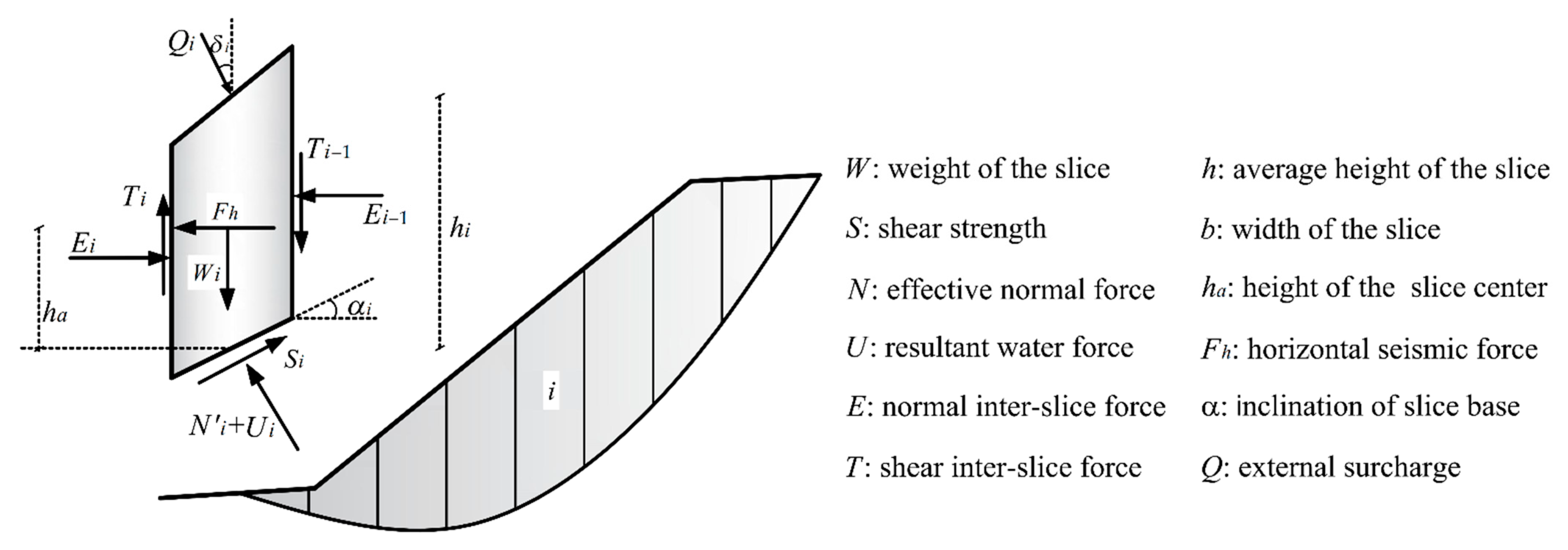
where K_h stands for horizontal acceleration coefficient, a_h stands for lateral ground motions, and g stands for gravity acceleration. The Morgenstern–Price model was used to analyze the safety factor under seismic load in this study. This method divides the sliding mass into a number of vertical segments, similar to other limit equilibrium techniques. Consider the loads applied to a standard slice of a slope, as displayed in Figure 1, with the overall shape of the slope.

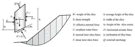
Figure 1. Forces acting on a typical slice.

The scaling factor (λ) and FOS are two unknown factors in the Morgenstern–Price method that are deduced from moment and vertical force equilibriums [63]. Because of the complexity of the obtained equations, evaluating the FOS and λ is often complicated. In order to solve the aforementioned challenges, Zhu et al. [64] developed a concise version of the Morgenstern–Price approach. In this concise method, the inclination of a resultant inter-slice pressure varies symmetrically with the mass of the slide, and the correlation between the shear (T) and normal (E) inter-slice forces is offered as follows:

T = f(x).λ.E

(2)

where f(x) denotes the assumed inter-slice force function, and λ denotes the scaling factor.

The following is a detailed description of the FOS evaluation procedure:

Step 1.

Create a trial slip surface and divide it into n vertical segments.

Step 2.

Determine R_i and T_i by using the equations below:

$$R_i=\left[W_i\cos {\alpha }_{i }+Q_i\cos \left({\delta }_i-{\alpha }_i\right)-F_h\sin {\alpha }_i-U_i\right]\times \tan {\varnothing }_i^{\prime }+c_i^{\prime }{b}_i\sec {\alpha }_{i }$$

(3)

$$T_i=F_h\cos {\alpha }_{i }+W_i\sin {\alpha }_i-Q_{i}sin\left({\delta }_i-{\alpha }_i\right)$$

(4)

Step 3.

Pick the function for inter-slice forces; f(x) = 1 is assumed in this study.

Step 4.

Consider FOS and λ initial amounts according to the following criteria:

$$\mathrm{FOS}>-\frac{\sin {\alpha }_i-\lambda f_i\cos {\alpha }_i}{\cos {\alpha }_i+\lambda f_i\sin {\alpha }_i}\tan {\varnothing }^{\prime }$$

(5)

The λ and FOS might be set to 0 and 1, respectively, as their initial values [64].

Step 5.

Evaluate Φ_i and $\mathsf{\Psi }$_i−1 based on Equations (6) and (7).

$${\mathsf{\Phi }}_i=\left(\cos {\alpha }_i+\lambda f_i\sin {\alpha }_i\right)\times \mathrm{FOS}+\left(\sin {\alpha }_i-\lambda f_i\cos {\alpha }_i\right)\tan {\varnothing }_i^{\prime }$$

(6)

$${\mathsf{\Psi }}_{i-1}=\left[\left(\sin {\alpha }_i-\lambda f_{i-1}\cos {\alpha }_i\right)\tan {\varnothing }_i^{\prime }+\left(\cos {\alpha }_i+\lambda f_{i-1}\sin {\alpha }_i\right)\times \mathrm{FOS}\right]/{\mathsf{\Phi }}_{i-1}$$

(7)

Step 6.

Calculate FOS based on Equation (8):

$$\mathrm{FOS}=\frac{{{\displaystyle \sum }}_{i=1}^{n-1}\left(R_i{{\displaystyle \prod }}_{j=1}^{n-1}{\mathsf{\Psi }}_j\right)+R_n}{{{\displaystyle \sum }}_{i=1}^{n-1}\left(T_i{{\displaystyle \prod }}_{j=1}^{n-1}{\mathsf{\Psi }}_j\right)+T_n}$$

(8)

Step 7.

Compute Φ_i and $\mathsf{\Psi }$_i−1 and calculate FOS once more by performing Steps 5 and 6 again.

Step 8.

Define E_i and λ based on the Equations (9) and (10).

$$E_i{\mathsf{\Phi }}_i=\mathrm{FOS}\times T_i-R_i+{\mathsf{\Psi }}_{i-1}{E}_{i-1}{\mathsf{\Phi }}_{i-1}$$

(9)

$$\lambda =\frac{{{\displaystyle \sum }}^{ }\left[b_i\left(E_i+E_{i-1}\right)\tan {\alpha }_i+F_h{h}_i+2Q\sin {\delta }_i{h}_i\right]}{{{\displaystyle \sum }}^{ }\left[b_i\left(f_i{E}_i+f_{i-1}{E}_{i-1}\right)\right]}$$

(10)

Step 9.

Reevaluate FOS by using the obtained λ, and this process ends when the distinction between the found FOS and λ falls below 0.005 and 0.01, respectively. For the analysis in this paper, the generation failure surface approach developed by Cheng et al. [65] was implemented for the general form of the failure surface, which divides the assumed failure soil mass into some vertical sections of equal width.

3. Proposed Chaotic Sand Cat and Pattern Search

3.1. Sand Cat Optimization

The sand cat optimization (SCO) method is named according to a unique feature of sand cat behavior in the environment that is the capacity to identify low-frequency sounds [60]. Foraging and attacking the prey are the two major behaviors of the sand cat. Based on the scientific research, the sand cat’s frequency absorption for frequencies below 2 kHz is amazing. Sand cats are around 8 decibels more sensitive than house cats at this frequency [66]. Because of these unique traits, the sand cat can detect sound (prey movement), follow prey, and hunt successfully based on prey position.

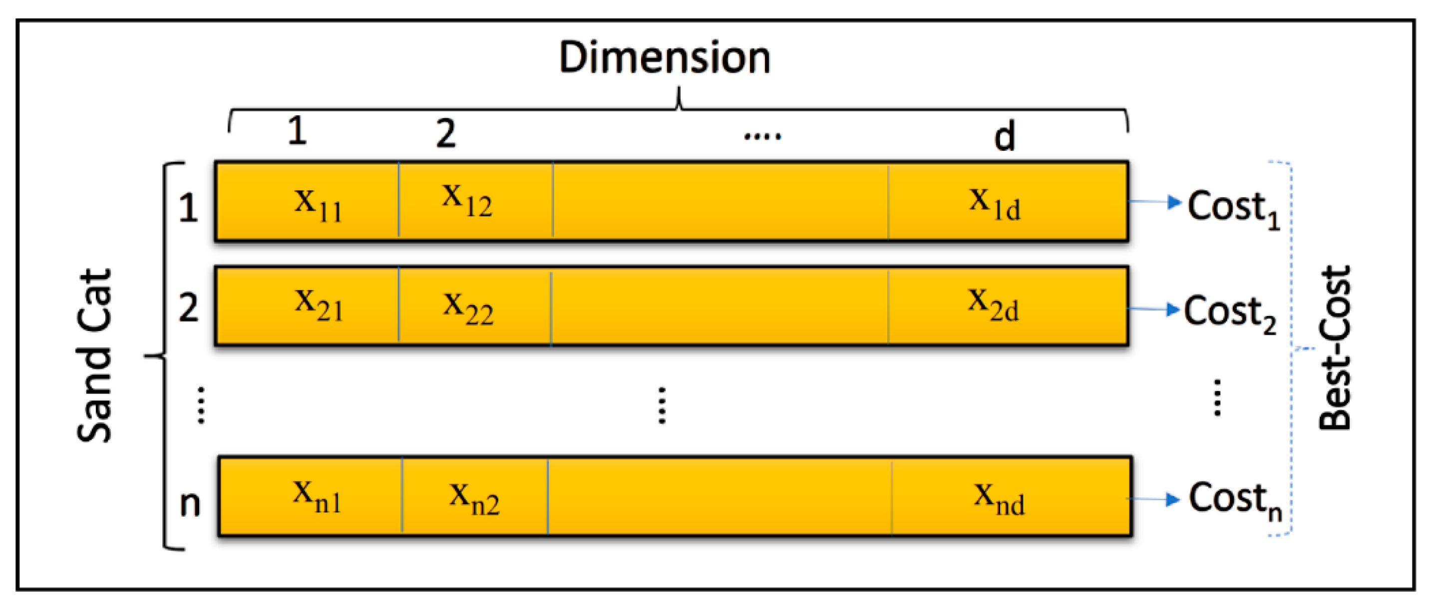
Each sand cat in the SCO algorithm represents a problem variable. To begin the SCO method, the candidate matrix of the sand cat population is generated randomly between the lower and higher limits of design variables. The dimension of the candidate matrix for a d-dimensional optimization space with n sand cats is equal to N_pop × N_d, (pop = 1, …, n), as shown in Figure 2.

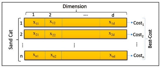
Figure 2. Initial candidate matrix generation.

Furthermore, the fitness value (i.e., cost) of each sand cat is calculated by using a specific fitness function. Each sand cat (i.e., candidate solution) will produce a value for the corresponding function. Once an iteration is completed, the sand cat with the lowest value in that iteration is picked as the best solution, and the other candidates (i.e., sand cats) strive to migrate toward this best-chosen cat in the following iteration.

Each sand cat’s solution is denoted by X_i = (x_i1, x_i2, …, x_id), (i = 1, …, n). The SCO algorithm takes advantage of the sand cat’s low-frequency hearing capabilities. As previously stated, the sand cat can detect frequencies below 2 kHz. As a result, it is hypothesized that the sensitivity range of a sand cat starts at 2 kHz and ends at 0 kHz when searching for prey. To represent this mechanism, and in mathematical simulation of the algorithm, the vector $\overrightarrow{r_G}$ is introduced that will linearly decrease from two to zero as the iterations increase according to the following equation [60]:

$$\overrightarrow{r_G}=S_M-\left(\frac{S_M\times t}{t_{Max}}\right)$$

(11)

The S_M value is supposed to be 2 since it is based on the hearing characteristics of sand cats [60]. Moreover, t represents the current iteration, and t_Max is the maximum number of iterations.

During the search phase, the position of each search agent is updated by using the following equation based on the best-candidate position ($\overrightarrow{Po{s}_b}$), its current position ($\overrightarrow{Po{s}_c}$), and its sensitivity range ($\overrightarrow{r}$).

$$\overrightarrow{Pos} \left(t+1\right)=\overrightarrow{r}·\left( \overrightarrow{Po{s}_b}\left(t\right)-rand\left(0, 1\right)·\overrightarrow{Po{s}_c}\left(t\right)\right)$$

(12)

To escape the local optimal trap, each sand cat has a separate sensitivity range ($\overrightarrow{r}$), which is calculated by using Equation (13).

$$\overrightarrow{r}=\overrightarrow{r_G}\times rand\left(0, 1\right)$$

(13)

As a result, $\overrightarrow{r_G}$ denotes the general sensitivity range, which is linearly reduced from 2 to 0. Furthermore, $\overrightarrow{r}$ shows the sensitivity range of each cat [60].

After searching, and in the attacking stage of SCO, each sand cat’s position is updated based on the following equation [60]:

$$\overrightarrow{Pos} \left(t+1\right)=\overrightarrow{Po{s}_b}\left(t\right)-\overrightarrow{r}·\overrightarrow{Po{s}_{rnd}}·\cos \left(\theta \right)$$

(14)

where θ is a random angle between 0 and 360, and $\overrightarrow{Po{s}_{rnd}}$ indicates the position of a randomly selected sand cat based on the following equation:

$$\overrightarrow{Po{s}_{rnd}}=\left|rand\left(0, 1\right)· \overrightarrow{Po{s}_b}\left(t\right)-\overrightarrow{Po{s}_c}\left(t\right)\right|$$

(15)

Finally, the R parameter, which is determined from Equation (16), is the last and most important parameter of the algorithm in determining the transition between exploration (searching) and exploitation (attacking) phases [60].

$$\overrightarrow{R}=2\times \overrightarrow{r_G}\times rand\left(0, 1\right)-\overrightarrow{r_G}$$

(16)

When R is less than or equal to 1, the SCO algorithm pushes the search agents to exploit; otherwise, they are driven to explore and discover prey [60]. Therefore, Equation (17) represents the final updating position equation of the SCO algorithm [60].

$$\overrightarrow{X}\left(t+1\right)=\{\begin{array}{c}\overrightarrow{Po{s}_b}\left(t\right)-\overrightarrow{Po{s}_{rnd}}\left(t\right)·\cos \left(\theta \right)·\overrightarrow{r} \left|R\right|\le 1;exploitation\\ \overrightarrow{r}·\left(\overrightarrow{Po{s}_b}\left(t\right)-rand\left(0, 1\right)·\overrightarrow{Po{s}_c}\left(t\right)\right) \left|R\right|>1;exploration\end{array}.$$

(17)

As presented in Equation (17), sand cats are ordered to attack their victim when |R| ≤ 1; otherwise, the cats are charged with seeking a new feasible solution in the global region. Algorithm 1 contains the pseudocode for the sand cat optimization (SCO).

Algorithm 1. Sand cat optimization algorithm.

Initialize the population Calculate the fitness function based on the objective function Initialize the r, rG, R While (t ≤ tMax)          For each sand cat                 Get a random angle θ ($0^{°}\le \theta \le {360}^{°})$                 If (|R| ≤ 1)  Update the search agent based on exploitation part of Equation (17); $\overrightarrow{Po{s}_b}\left(t\right)-\overrightarrow{Po{s}_{rnd}}\left(t\right)·\cos \left(\theta \right)·\overrightarrow{r}$                Else  Update the search agent based on the exploration part of Equation (17); $\overrightarrow{r·}\left(\overrightarrow{Po{s}_b}\left(t\right)-rand\left(0, 1\right)·\overrightarrow{Po{s}_c}\left(t\right)\right)$                End       End     t = t+1 End

3.2. Chaotic Sand Cat Optimization

The present study’s goal is to put the SCO’s global search capability into practice. Therefore, the chaotic series is employed in the sensitivity range parameter of Equation (13) to achieve this goal and to expand the algorithm’s exploring capacity. Chaotic phenomena are deterministic systems with unpredictability, irregularity, and stochastic features that are influenced by the initial circumstances. Chaotic parameters have the capability to fluctuate across certain limits due to their inherent irregularity without repeating. A chaotic record is one that displays some sort of chaotic pattern and can generate chaotic movement. The well-known logistic map is used in this work, which is in accordance with the following equation:

µ (t+1) = a × µ (t) × (1 − µ (t))

(18)

where µ (t) denotes the chaotic map; t shows the iteration number; a represents a constant equivalent to 4; and µ (0) should be between 0 and 1 and not equal to 0, 0.25, 0.5, 0.75, or 1.

In the chaotic SCO (CSCO), the chaotic map µ is utilized instead of a simple random number in the sensitivity range ($\overrightarrow{r}$) evaluation equation (i.e., Equation (13)) to enhance the algorithm’s stochastic behavior while preventing premature convergence. Therefore, the position of a sand cat will be updated based on the following equation:

$$\overrightarrow{X}\left(t+1\right)=\{\begin{array}{c}\overrightarrow{Po{s}_b}\left(t\right)-\overrightarrow{Po{s}_{rnd}}\left(t\right)·\cos \left(\theta \right)·\overrightarrow{r_G}\times \mu \left|R\right|\le 1;exploitation\\ \overrightarrow{r_G}\times \mu ·\left(\overrightarrow{Po{s}_{bc}}\left(t\right)-rand\left(0,1\right)·\overrightarrow{Po{s}_c}\left(t\right)\right) \left|R\right|>1;exploration\end{array}$$

(19)

Furthermore, in the suggested CSCO, to enhance the algorithm’s exploration and search capability, at every iteration, the poorest sand cat offering the highest fitness value (in minimization problems) will be changed by a new one, as presented in the following equation:

$$x_{worst}=\{\begin{array}{c}ran{d}_1\times \overrightarrow{Po{s}_b}\left(t\right) if ran{d}_3\le 0.5\\ x_{i min}+ran{d}_2\times \left(x_{i max}-x_{i min}\right) if ran{d}_3>0.5\end{array}$$

(20)

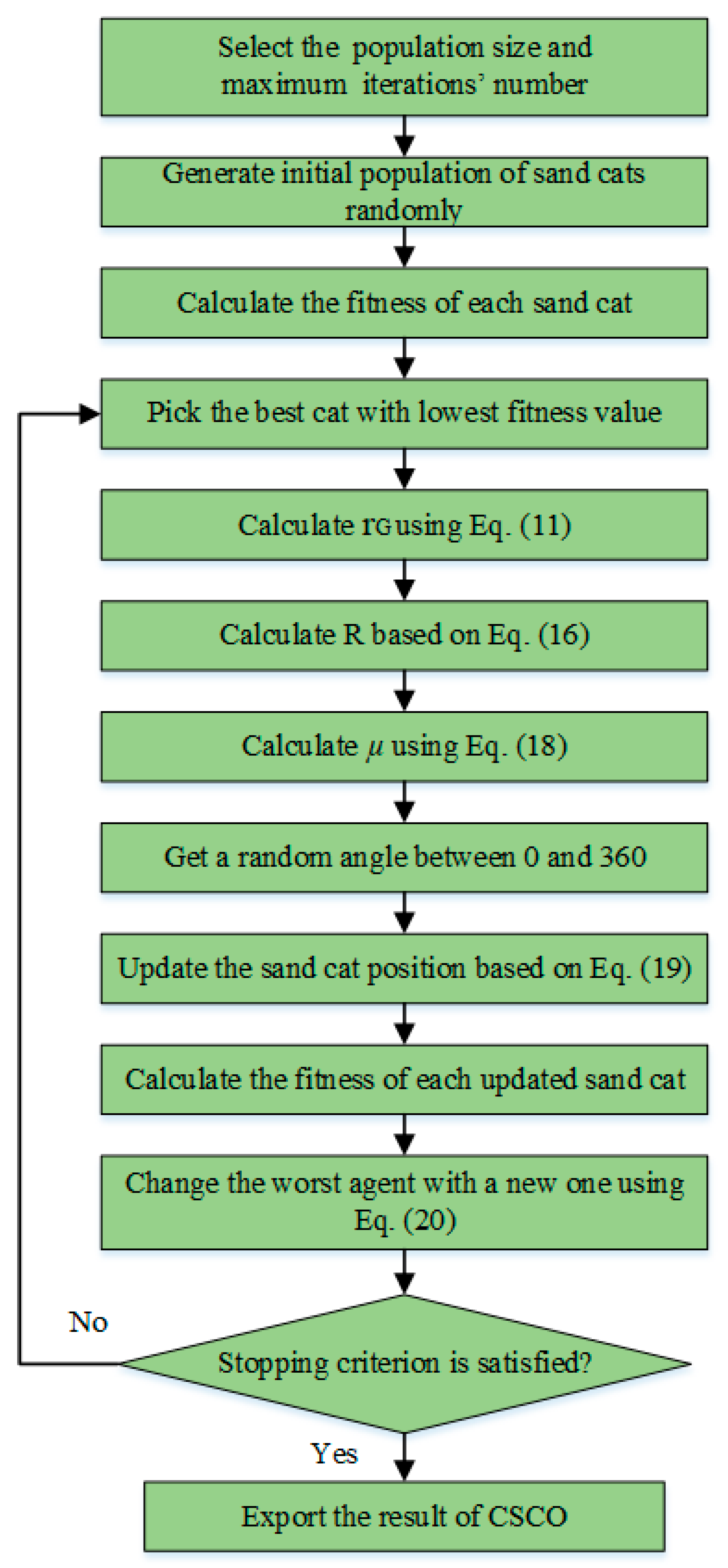
where $x_{worst}$ is a sand cat with the highest fitness value; and $ran{d}_1$, $ran{d}_2$, and $ran{d}_3$ are random values between 0 and 1. The procedure of the proposed chaotic sand cat is depicted in Figure 3.

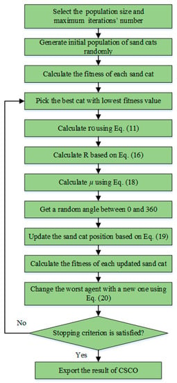
Figure 3. Chaotic sand cat optimization algorithm.

3.3. Pattern Search (PS)

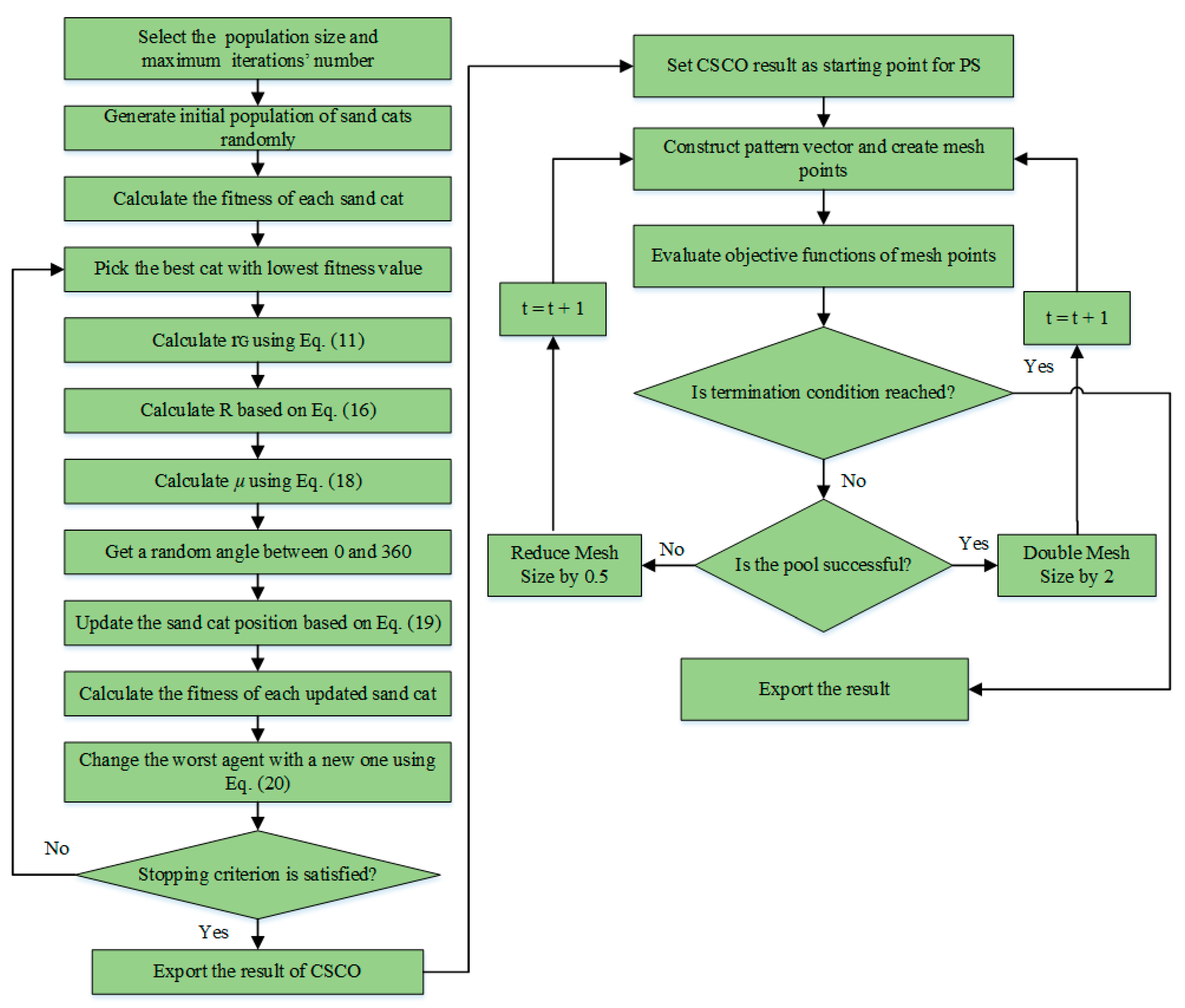
PS is a gradient-free approach for fine-tuning local search that can be easily implemented. The PS method produces a group of locations that may or may not be near the ideal point [67]. A mesh (a combination of elements) is formed around an existing element in the first round. In the next round, if a new element in the mesh has a smaller fitness, it becomes the current element.

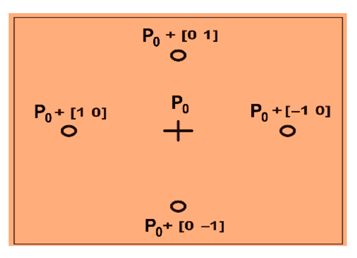
The PS commences the investigation with a user-defined initial location, P₀. The mesh level is taken as 1 in the first round, and the pattern elements are generated as [0 1] + P₀, [1 0] + P₀, [−1 0] + P₀, and [0 −1] + P₀, and novel mesh elements are added as depicted in Figure 4. The fitness function is then computed for each created sample element until a value less than P₀ is discovered. The poll is successful if there is such an element (f (P₁) < f (P₀)), and the PS method assumes this element as the basis point.

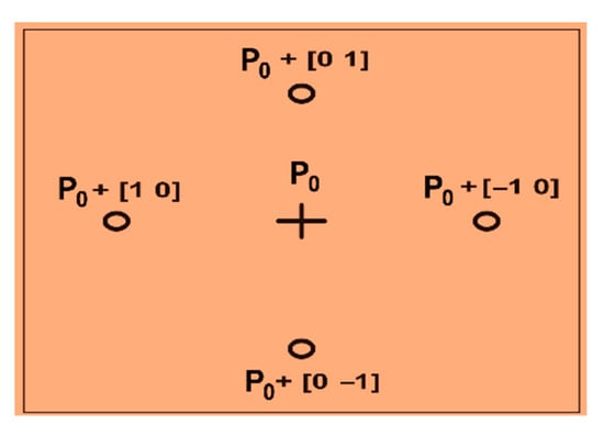
Figure 4. Pattern-search mesh elements.

After a positive poll, the technique advances to the second round and doubles the current mesh size by two (known as the expanding factor) with the following new elements: 2 × [0 1] + P₁, 2× [1 0] + P₁, 2 × [−1 0] +P₁, and 2 × [0 −1] + P₁. Then P₂ is established if a value less than P₁ is discovered, the mesh size is expanded by two, and iterations proceed.

The existing element is left alone, and the mesh size is decreased by a contraction factor if the poll is unsuccessful at any round. These steps were continued until the lowest value was reached or the termination criteria were fulfilled.

A hybrid approach is one that solves the same issue by combining two or more methods. The goal of hybridization is to integrate the benefits of each method to improve the result’s precision [68]. In the current research, the chaotic sand cat—pattern search (CSCPS) approach, which combines chaotic sand cat and pattern search methods, was developed. The chaotic sand cat is a global optimization technique that investigates the solution space effectively and is likely to provide an optimum or near-optimal solution. As a result, it may be used in conjunction with local optimization approaches such as pattern search. Pattern search is useful for exploiting a small area, but it is rarely useful for exploring a larger area. The suggested hybrid approach may take the CSCO’s powerful global searching capabilities, as well as the PS algorithm’s strong local searching capabilities.

3.4. Chaotic Sand Cat–Pattern Search

The global optimum performance of chaotic sand cat optimization (CSCO) is excellent, and it is easy to get out of local minima. The CSCO can increase the precision of the results by raising the number of iterations. However, CSCO seems unable to enhance the precision of the findings when the number of epochs is sufficiently high. Consequently, CSCO’s local investigation power remains poor. The starting point significantly affects the results of the pattern search algorithm, which uses a local optimization methodology and different initial points resulting in significant differences in the outcomes. However, even so, pattern search will be a quick and efficient tactic if a great starting point is selected. In this study, we successfully combined the benefits of CSCO as a global optimization and pattern search as a local optimization to identify the best answer. Because the PS is dependent on the first solution, the suggested hybrid method starts with the CSCO. The CSCO is used to keep searching for a certain number of iterations. The PS is then enabled to perform a local search utilizing the CSCO’s best solution as an initial point. Figure 5 shows the process flow of the suggested hybrid algorithm.

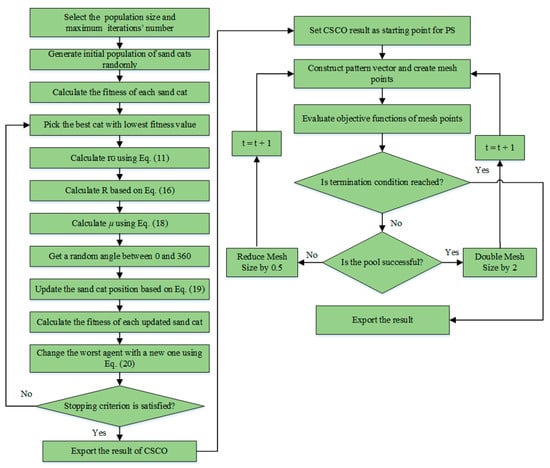
Figure 5. Hybrid chaotic sand cat–pattern search algorithm.

4. Model Verification

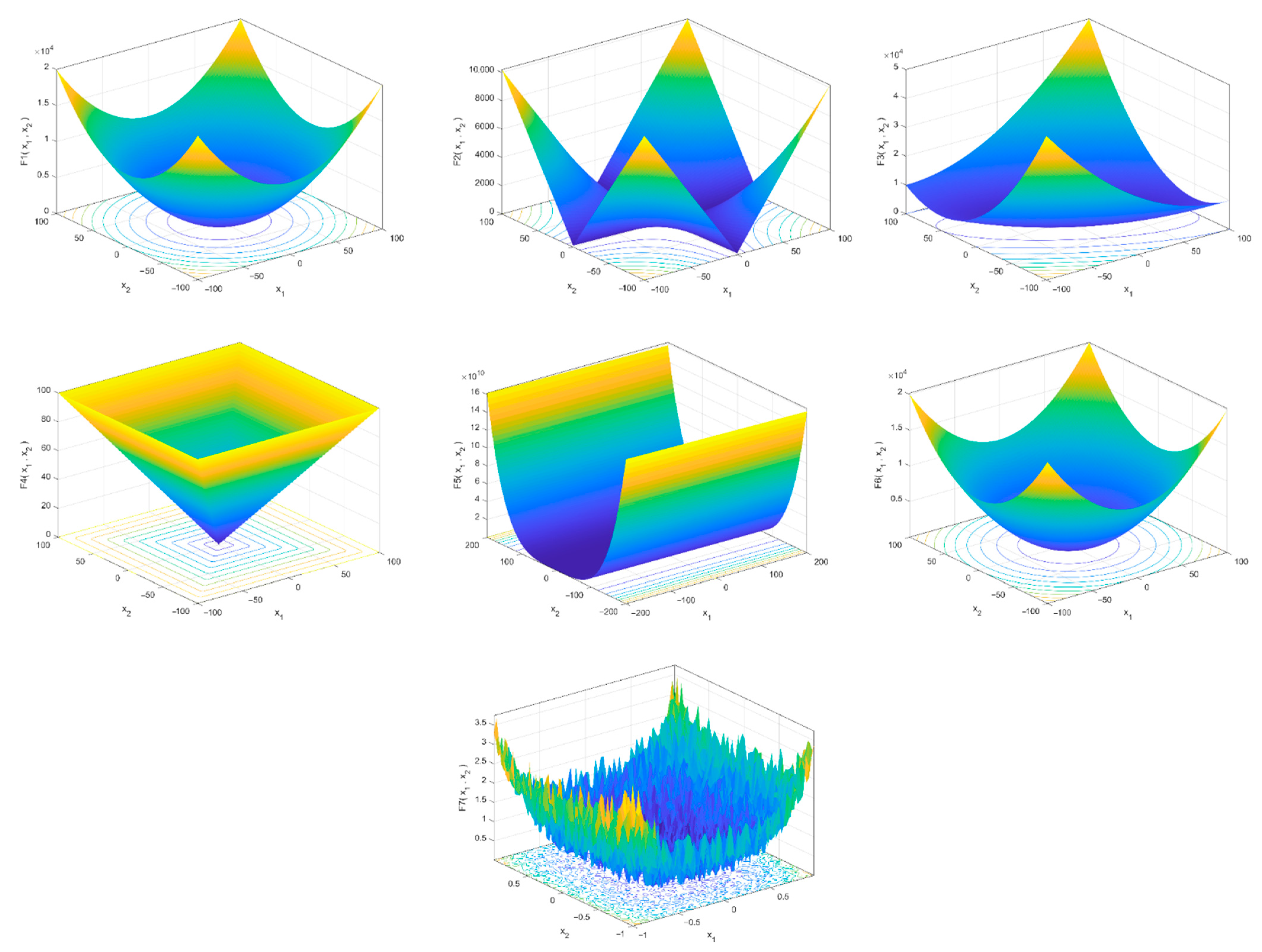
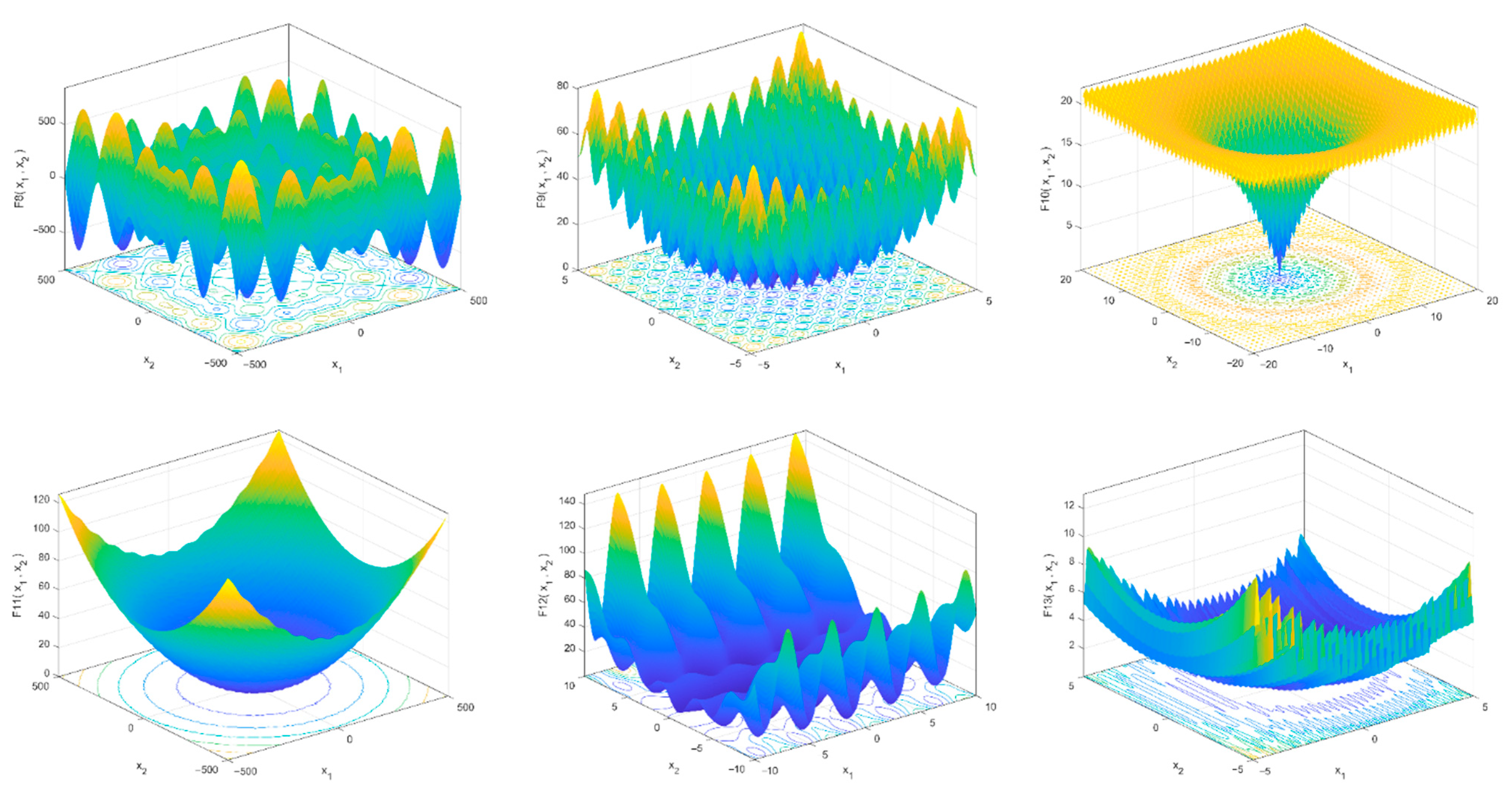
In this section, we recount how a set of numerical reference test functions was used to compare and confirm the effectiveness of the proposed chaotic sand cat–pattern search algorithm (CSCPS). In the empirical-evidence literature, these functions are commonly used to determine the performance of optimization algorithms [69,70]. The mathematical model and characteristics of these test functions are shown in Table 2 and Table 3. This standard set is divided into two categories: the exploitation ability of an algorithm was examined by using unimodal functions with a single global best; and the multi-modal functions were examined with multiple local minimums for testing an algorithm’s capability for exploring and avoiding local optima. MATLAB R2020b (Natick, MA, USA) was used to create the suggested algorithms. All of these functions should be minimized. Furthermore, all functions have a dimension of 30. Three-dimensional drawings of these benchmark functions are illustrated in Figure 6 and Figure 7.

Table 2. Unimodal functions.

Function	Range	${\mathit{f}}_{\mathit{m}\mathit{i}\mathit{n}}$	n (Dim)
$F_1\left(X\right)={\displaystyle \sum }_{i=1}^n{x}_i^2$	${\left[-100, 100\right]}^n$	0	30
$F_2\left(X\right)={\displaystyle \sum }_{i=1}^n\left|x_i\right|+{\displaystyle \prod }_{i=1}^n\left|x_i\right|$	${\left[-10, 10\right]}^n$	0	30
$F_3\left(X\right)={\displaystyle \sum }_{i=1}^n{\left({\displaystyle \sum }_{j=1}^i{x}_j\right)}^2$	${\left[-100, 100\right]}^n$	0	30
$F_4\left(X\right)=\underset{i}{\max } \left\{\left|x_i\right|, 1\le i\le n \right\}$	${\left[-100, 100\right]}^n$	0	30
$F_5\left(X\right)={\displaystyle \sum }_{i=1}^{n-1}\left[100{\left(x_{i+1}-x_i^2\right)}^2+{\left(x_i-1\right)}^2\right]$	${\left[-30, 30\right]}^n$	0	30
$F_6\left(X\right)={\displaystyle \sum }_{i=1}^n{\left(\left[x_i+0.5\right]\right)}^2$	${\left[-100, 100\right]}^n$	0	30
$F_7\left(X\right)={\displaystyle \sum }_{i=1}^{n}i{x}_i^4+random\left[0, 1\right)$	${\left[-1.28, 1.28\right]}^n$	0	30

Table 3. Multimodal functions.

Function	Range	${\mathit{f}}_{\mathit{m}\mathit{i}\mathit{n}}$	n (Dim)
$F_8\left(X\right)={\displaystyle \sum }_{i=1}^n-x_i\sin \left(\sqrt{\left|x_i\right|}\right)$	${\left[-500, 500\right]}^n$	428.9829 × n	30
$F_9\left(X\right)={\displaystyle \sum }_{i=1}^n\left[x_i^2-10\cos \left(2\pi x_i\right)+10\right]$	${\left[-5.12, 5.12\right]}^n$	0	30
$F_{10}\left(X\right)=-20 \exp \left(-0.2\sqrt{\frac{1}{n}{\displaystyle \sum }_{i=1}^n{x}_i^2}\right)-exp\left(\frac{1}{n}{\displaystyle \sum }_{i=1}^n\cos \left(2\pi x_i\right)\right)+20+e$	${\left[-32, 32\right]}^n$	0	30
$F_{11}\left(X\right)=\frac{1}{4000}{\displaystyle \sum }_{i=1}^n{x}_i^2-{\displaystyle \prod }_{i=1}^n\cos \left(\frac{x_i}{\sqrt{i}}\right)+1$	${\left[-600, 600\right]}^n$	0	30
$F_{12}\left(X\right)=$  $\frac{\pi }{n}\left\{10\sin \left(\pi y_1\right)+{\displaystyle \sum }_{i=1}^{n-1}{\left(y_i-1\right)}^2\left[1+10{\sin }^2\left(\pi y_{i+1}\right)\right]+{\left(y_n-1\right)}^2\right\}+{\displaystyle \sum }_{i=1}^{n}u\left(x_i,10, 100, 4\right)$ $y_i=1+\frac{x_{i+4}}{4}$ $u\left(x_i,a, k, m\right)=\{\begin{array}{c}k{\left(x_i-a\right)}^m x_i>a \\ 0 a< x_i<a \\ k{\left(-x_i-a\right)}^m x_i<-a\end{array}$	${\left[-50, 50\right]}^n$	0	30
$F_{13}\left(X\right)=0.1\left\{{\sin }^2\left(3\pi x_1\right)+{\displaystyle \sum }_{i=1}^n{\left(x_i-1\right)}^2\left[1+{\sin }^2\left(3\pi x_i+1\right)\right]+{\left(x_n-1\right)}^2\left[1+{\sin }^2\left(2\pi x_n\right)\right]\right\}+{\displaystyle \sum }_{i=1}^{n}u\left(x_i,5, 100, 4\right)$	${\left[-50, 50\right]}^n$	0	30

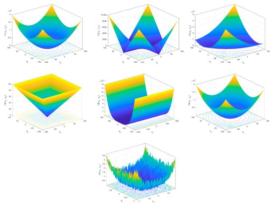
Figure 6. Three-dimensional plots of unimodal test functions.

Figure 7. Three-dimensional plots of multimodal test functions.

The proposed CSCPS is compared to the original SCO, as well as some well-known optimization methods, such as particle swarm optimization (PSO) proposed by Reference [71], firefly algorithm (FA) introduced by Reference [72], multi-verse optimizer (MVO) developed by Reference [73], tunicate swarm algorithm (TSA) introduced by Reference [70], and salp swarm algorithm (SSA). For all methodologies, the size of solutions (N) and the maximum number of iterations (t_max) are set to 30 and 1000, respectively, in order to make a fair comparison between them.

Because the results of a single run of metaheuristic methods are stochastic, they may be incorrect. As a result, statistical analysis should be performed in order to provide a fair comparison and evaluate the algorithms’ efficacy. To address this issue, 30 time runs for the mentioned methods were performed, with the results presented in Table 4 and Table 5.

Table 4. Results comparison of unimodal functions.

F	Index	CSCPS	SCO	PSO	FA	MVO	SSA	TSA
F1	Mean	0.00	2.42 × 10−97	4.98 × 10−9	7.11 × 10−3	2.81 × 10−1	3.29 × 10−7	8.31 × 10−56
	SD	0.00	7.22 × 10−97	1.40 × 10−8	3.21 × 10−3	1.11 × 10−1	5.92 × 10−7	1.02 × 10−58
F2	Mean	0.00	1.16 × 10−52	7.29 × 10−4	4.34 × 10−1	3.96 × 10−1	1.9111	8.36 × 10−35
	SD	0.00	2.55 × 10−52	1.84 × 10−3	1.84 × 10−1	1.41 × 10−1	1.6142	9.86 × 10−35
F3	Mean	0.00	7.84 × 10−81	1.40 × 10	1.66 × 103	4.31 × 10	1.50 × 103	1.51 × 10−14
	SD	0.00	3.49 × 10−80	7.13	6.72 × 102	8.97	707.05	6.55 × 10−14
F4	Mean	0.00	4.57 × 10−46	6.00 × 10−1	1.11 × 10−1	8.80 × 10−1	2.44 × 10−5	1.95 × 10−5
	SD	0.00	9.98 × 10−46	1.72 × 10−1	4.75 × 10−2	2.50 × 10−1	1.89 × 10−5	4.49 × 10−4
F5	Mean	7.22 × 10−8	2.80 × 10	4.93 × 10	7.97 × 10	1.18 × 102	136.56	28.4
	SD	4.78 × 10−9	8.73 × 10−1	3.89 × 10	7.39 × 10	1.43 × 102	154.00	0.842
F6	Mean	0.00	2.15	6.92 × 10−2	6.94 × 10−3	2.02 × 10−2	5.72 × 10−7	3.67
	SD	0.00	4.47 × 10−1	2.87 × 10−2	3.61 × 10−3	7.43 × 10−3	2.44 × 10−7	0.3353
F7	Mean	1.39 × 10−5	1.51 × 10−4	8.94 × 10−2	6.62 × 10−2	5.24 × 10−2	8.82 × 10−5	0.0018
	SD	2.65 × 10−5	1.33 × 10−4	0.0206	4.23 × 10−2	1.37 × 10−2	6.94 × 10−5	4.62 × 10−4

Table 5. Results comparison of multimodal functions.

F	Index	CSCPS	SCO	PSO	FA	MVO	SSA	TSA
F8	Mean	−1.25 × 104	−1.01 × 104	−6.01 × 103	−5.85 × 103	−6.92 × 103	−7.46 × 103	−7.89 × 103
	SD	0.00	1.70 × 103	1.30 × 103	1.61 × 103	9.19 × 102	634.67	599.26
F9	Mean	0.00	0.00	4.72 × 10	1.51 × 10	1.01 × 102	55.45	151.45
	SD	0.00	0.00	1.03 × 10	1.25 × 10	1.89 × 10	18.27	35.87
F10	Mean	8.88 × 10−16	8.77 × 10−16	3.86 × 10−2	4.58 × 10−2	1.15	2.84	2.409
	SD	0.00	0.00	2.11 × 10−1	1.20 × 10−2	7.87 × 10−1	6.58 × 10−1	1.392
F11	Mean	0.00	0.00	5.50 × 10−3	4.23 × 10−3	5.74 × 10−1	2.29 × 10−1	0.0077
	SD	0.00	0.00	7.39 × 10−3	1.29 × 10−3	1.12 × 10−1	1.29 × 10−1	0.0057
F12	Mean	1.57 × 10−32	1.25 × 10−1	1.05 × 10−2	3.13 × 10−4	1.27	6.82	6.373
	SD	2.88 × 10−48	5.41 × 10−2	2.06 × 10−2	1.76 × 10−4	1.02	2.72	3.458
F13	Mean	1.35 × 10−32	1.99	4.03 × 10−1	2.08 × 10−3	6.60 × 10−2	21.31	2.897
	SD	2.95 × 10−48	2.51 × 10−1	5.39 × 10−1	9.62 × 10−4	4.33 × 10−2	16.99	0.643

Table 4 and Table 5 show that, for all functions, the CSCPS might provide better solutions in terms of the mean value of the objective functions than the conventional SCO, as well as other optimization techniques. The results also show that the mean and standard deviation of the CSCPS algorithm are significantly lower than those of the other strategies, indicating that the algorithm is stable. According to the findings, the CSCPS outperforms both the standard method and alternative optimization approaches.

5. Model Application

The suggested CSCPS algorithm is employed for seismically slope stability issues in this section, according to the present study’s main goal. The Morgenstern–Price method was employed to determine the safety factor for static and earthquake stresses for a general form of failure surface. The suggested CSCPS algorithm is used to determine the critical failure associated with the minimum factor of safety. Two series of experiments from previous studies are used to evaluate the potential application and efficacy of the suggested research methods in finding the best FOS value. The number of predetermined slip surface slices is assumed to be 40 in both cases. The algorithm’s parameters are the same as in Section 4. All cases are remedied by taking into account three distinct values of K_h: 0.0, 0.1, and 0.2. Due to their stochastic nature, both algorithms (i.e., SCO and CSCPS) run 30 epochs autonomously for each problem, and the optimum outcomes are presented.

5.1. A Uniform Soil Slope

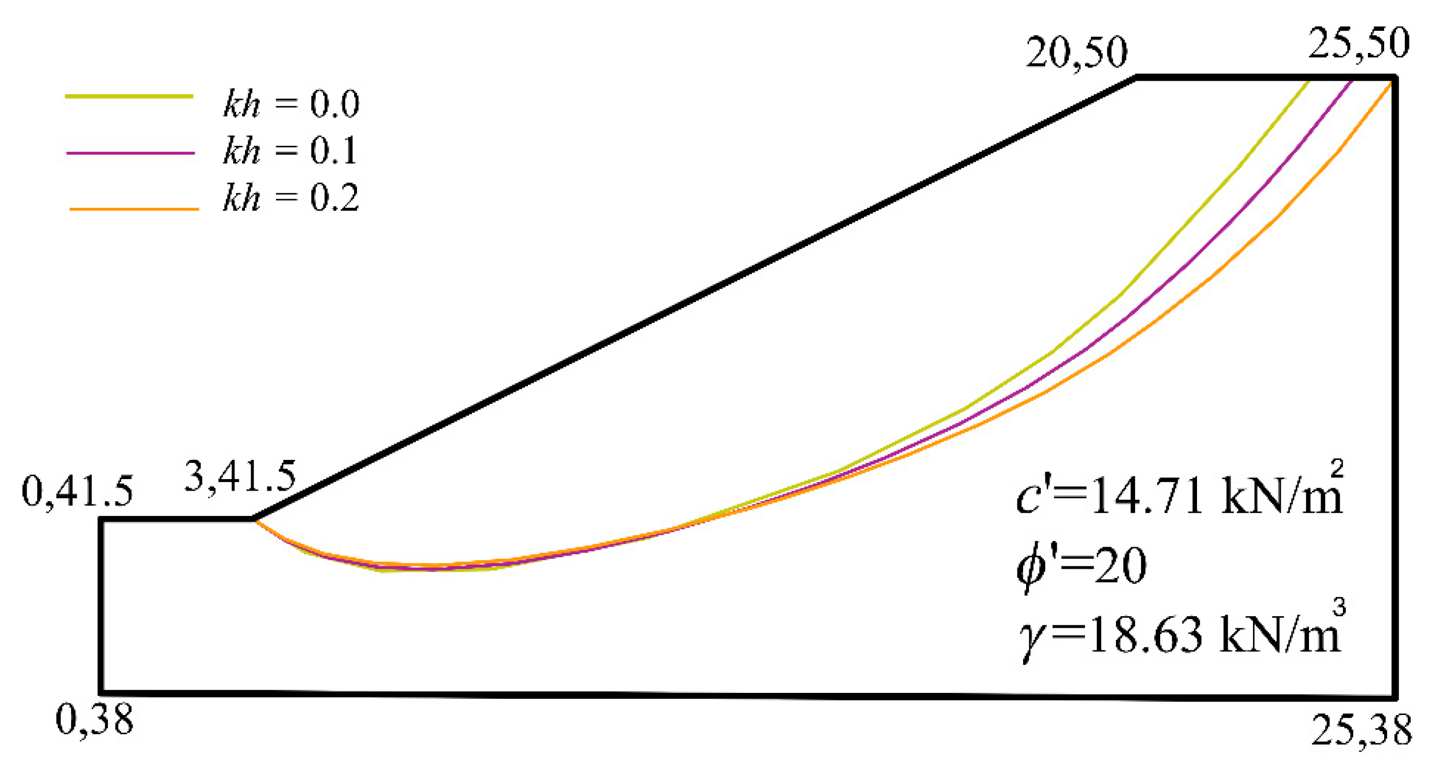
The primary case study is a dry slope in a relatively homogenous soil, which was studied by Zolfaghari et al. [6]. Figure 8 depicts the slope’s geometric design. The slope is 10.0 m high, with a steepness of 26.56 degrees. The soil’s effective friction angle (ϕ′) is 20°, its effective cohesiveness (c′) is 14.71 kPa, and its unit weight (γ) is 18.63 kN/m³.

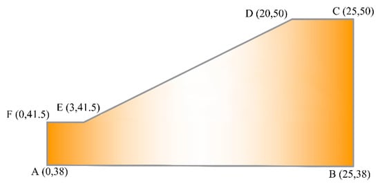
Figure 8. Slope in a uniform soil.

Zolfaghari et al. [6] solved this case by using a simple evolutionary genetic algorithm (GA) and the Morgenstern–Price method (2005). Cheng et al. [8] used six heuristic algorithms and Spencer’s technique to solve the problem and find the failure surface. They discovered that the harmony search (HS) and simulated annealing (SA) algorithms could outperform other approaches [8]. Finally, Himanshu and Burman [11] adopted particle swarm optimization (PSO) for the solution, as well as Bishop’s method. In the abovementioned research, the static load is considered. This condition is the same as Case 1 (K_h = 0) in the current study.

This case study is executed by utilizing the proposed CSCPS approach for various values of K_h, and the associated lowest factors of safety are computed and presented in Table 6. Table 6 shows that the minimum FOS calculated by the suggested CSCPS is 1.7132, which is lower than the FOS calculated by the other methodologies when K_h is zero. Furthermore, when compared to the standard method, the CSCPS algorithm could calculate better results for all loading cases.

Table 6. The best FOSs for slope in a uniform soil.

Optimization Method	Analysis Method	Number of Slices	Minimum FOS
			Kh = 0.0	Kh = 0.1	Kh = 0.2
GA [6]	Morgenstern–Price	-	1.75	_	_
SA [8]	Spencer’s method	40	1.7267	_	_
HS [8]	Spencer’s method	40	1.7264	_	_
PSO [11]	Bishop’s method	40	1.7195	_	_
SCO (current study)	Morgenstern–Price	40	1.7275	1.4012	1.1897
CSCPS (current study)	Morgenstern–Price	40	1.7132	1.3803	1.1424

The foregoing results indicate that CSCPS can reduce FOS and the critical failure surface associated with it, demonstrating its advantage. Furthermore, increasing the K_h to 0.1 and 0.2 reduces the FOS by 19 and 32 percent, respectively. Figure 9 shows the critical slip surfaces for each loading case.

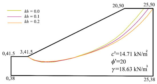
Figure 9. Critical failure surfaces for single-layered slope.

5.2. Slope in a Multi-Layered Soil

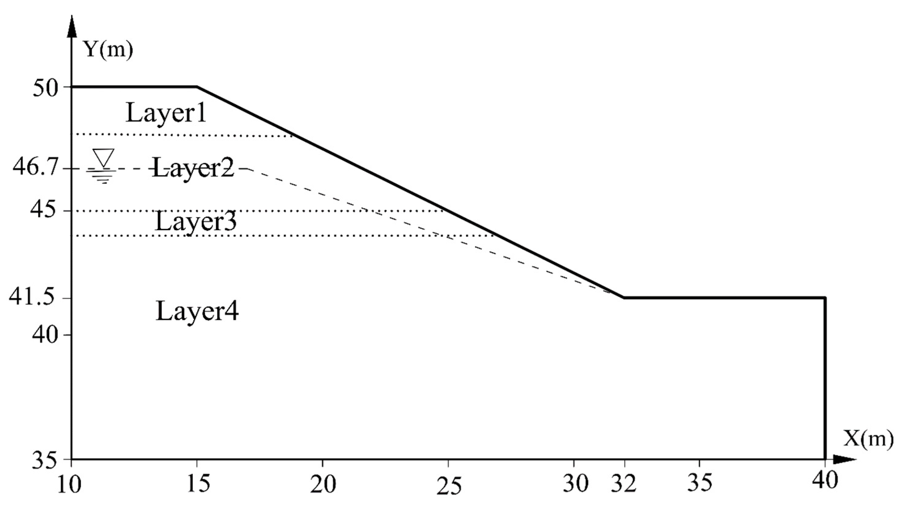
The next problem is a four-layer slope with different soil properties presented initially by Zolfaghri et al. [6]. Figure 10 displays the slope geometry, and the surface of the water is represented by a dashed line at an elevation of 46.7 m.

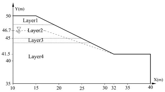
Figure 10. Multi-layered slope.

Table 7 contains the soil properties of each layer. For this case, Zolfaghari et al. [6] used an evolutionary genetic algorithm (GA) in conjunction with the Morgenstern–Price method by considering four different loading cases:

Table 7. Soil properties for multi-layered slope.

Soil Properties	Unit	Layer Number
		1	2	3	4
Unit weight, γ	kN/m3	18.63	18.63	18.63	18.63
Cohesion, c′	kPa	14.7	16.7	4.9	34.3
Friction angle, ϕ′	Degree	20	21	10	28

No flow of water and no seismic loads for Case 1; flow of water and no seismic loadings for Case 2; seismic load by K_h = 0.1 and no water flow for Case 3; and seismic load by K_h = 0.1 and water flow for Case 4.

This case is solved by utilizing the suggested CSCPS algorithm, and two additional loading conditions are considered in addition to the ones mentioned. No flow of water and seismic load with K_h = 0.2 as Case 5; water flow and seismic load with K_h = 0.2 as Case 6.

Cheng et al. [8] used six optimization approaches with the Spencer technique to solve this case and find the critical failure surface. According to their findings, when compared to other approaches, the PSO may provide a lower FOS value. The minimum factors of safety obtained in the previous studies and those calculated by the proposed methodology are tabulated in Table 8 for different load cases.

Table 8. The best FOSs for multi-layered slope.

Optimization Method	Analysis Method	Loading Case
		1	2	3	4	5	6
GA [6]	Morgenstern–Price	1.48	1.36	1.37	0.98	_	_
PSO [8]	Spencer method	1.3372	1.21	1.0474	0.9451	_	_
SCO (current study)	Morgenstern–Price	1.342	1.206	1.0546	0.985	0.849	0.69
CSCPS (current study)	Morgenstern–Price	1.322	1.178	1.019	0.916	0.814	0.657

Table 8 shows that the lowest FOS obtained by the suggested methodology is much lower than GA’s (nearly 10%) and slightly lower than PSO’s for all load cases. Based on the above findings, it can be found that the present CSCPS algorithm can be used to effectively evaluate the seismic stability of the slope.

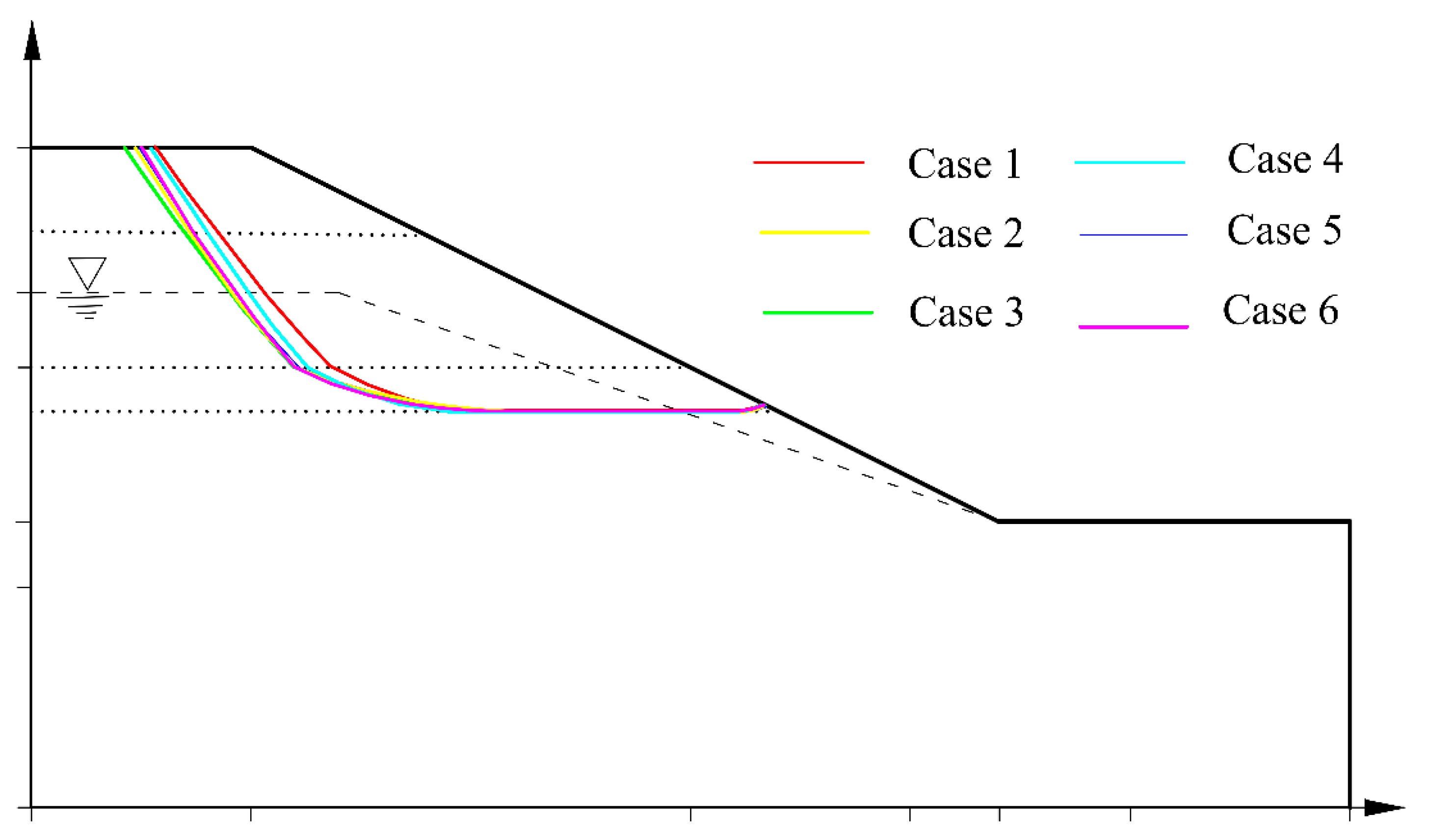
The critical slip surfaces connected to the lowest factors of safety for each loading condition obtained by the proposed method are presented graphically in Figure 11.

Figure 11. Critical failure surfaces for multi-layered slope.

6. Discussion

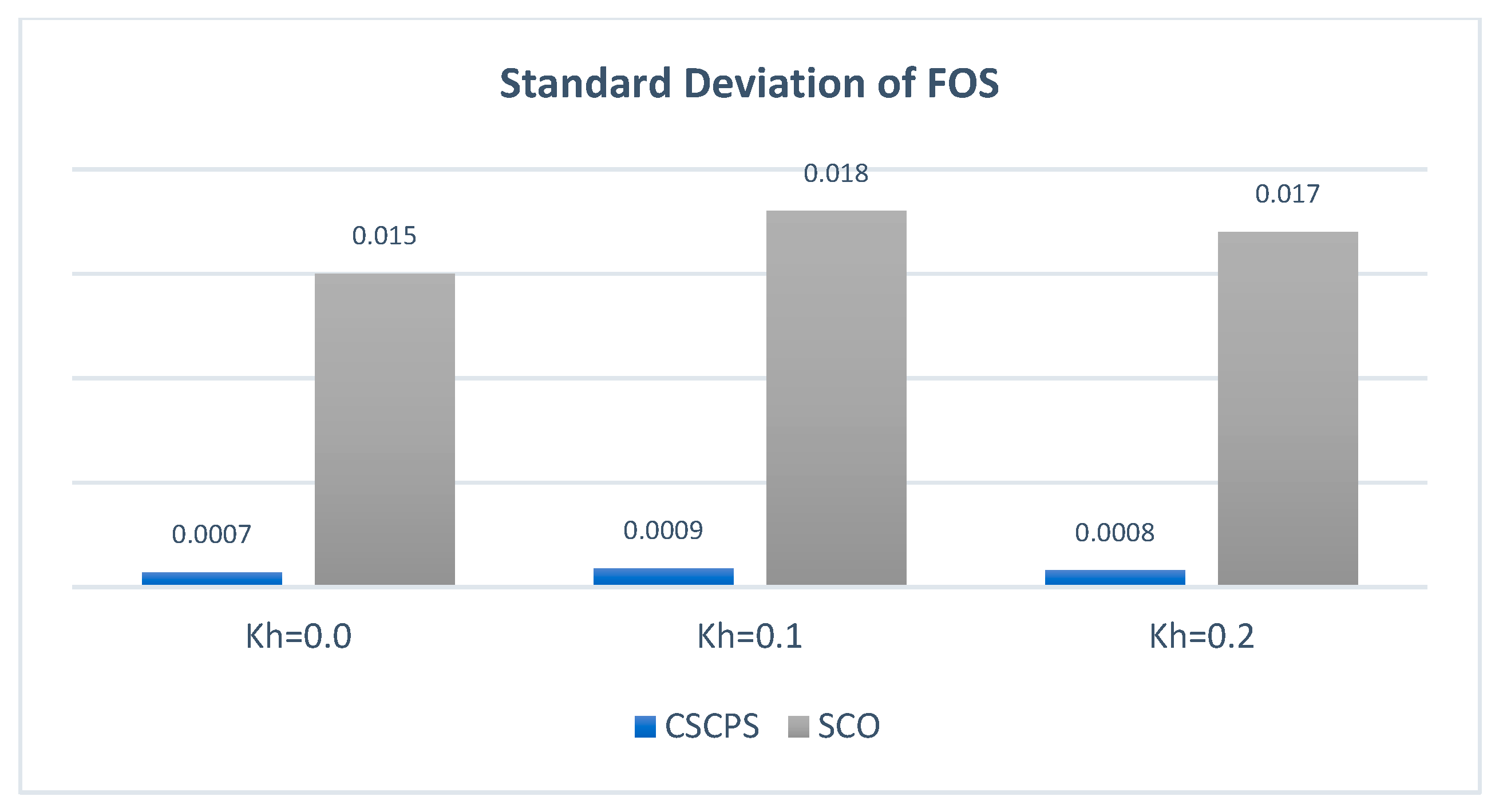
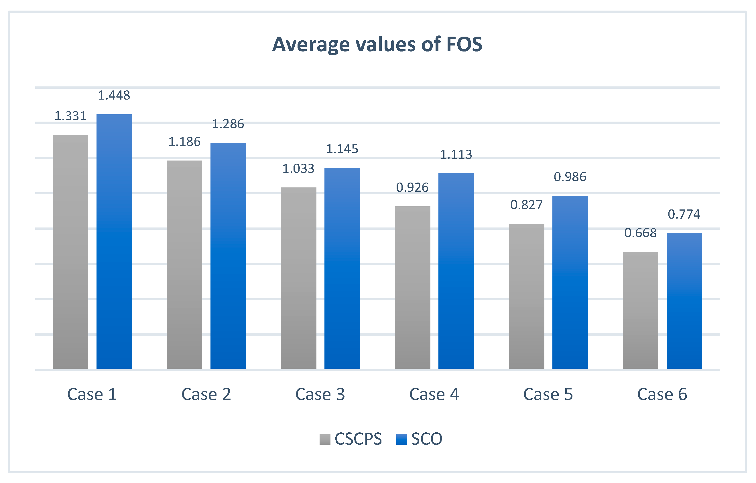
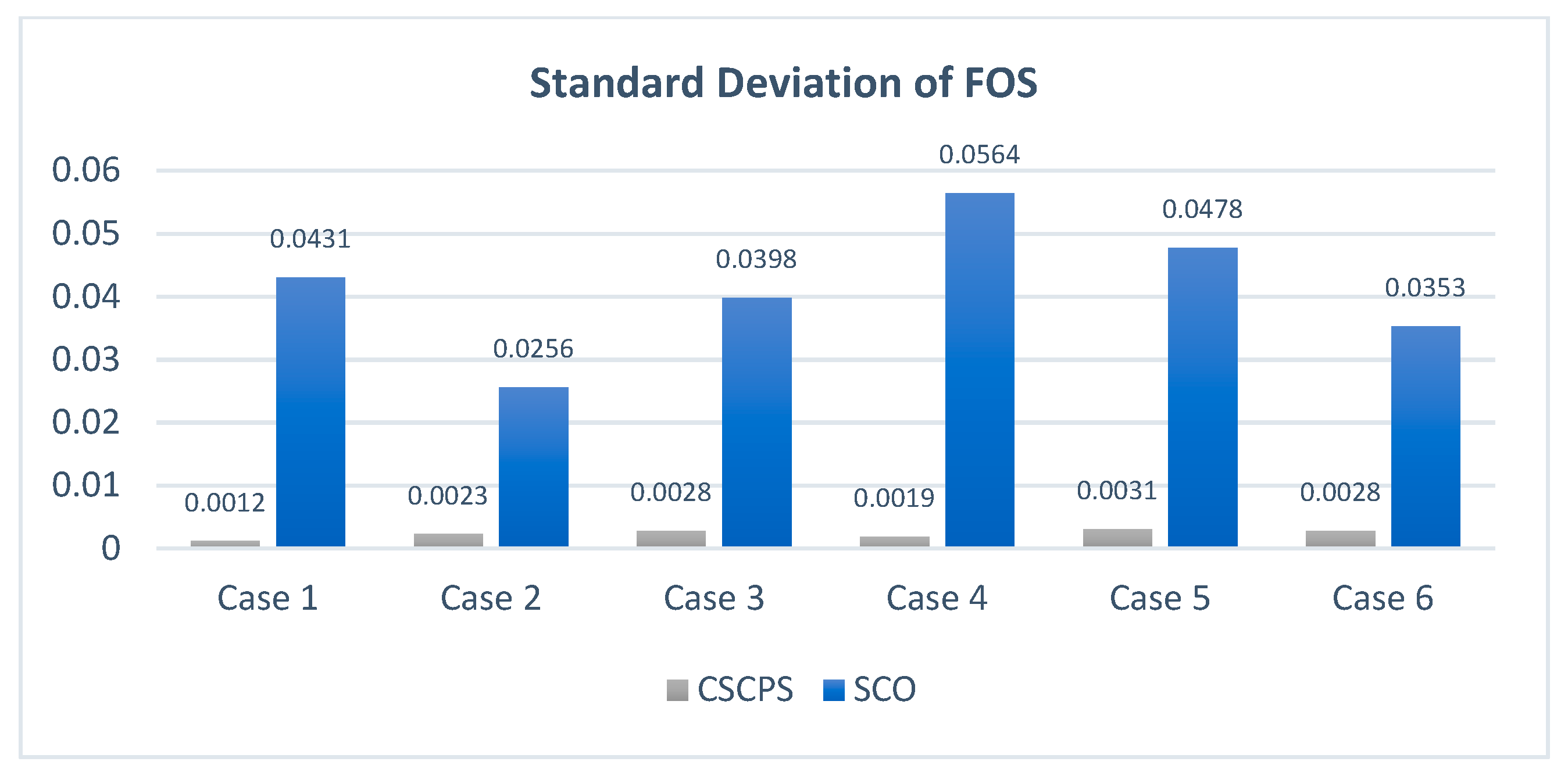
In the previous section, two case studies of slope stability problems were solved by using the proposed method, and the obtained results were compared with other approaches. The statistical analysis of the obtained results is presented in this section to discuss the efficiency of the proposed method. As mentioned in Section 6, because of the stochastic nature of SCO and CSCPS, both techniques were run 30 times, and the optimum result obtained by each method is reported. The FOS mean and standard deviation from 30 runs are shown in Figure 12 and Figure 13, respectively. Considering these results, the mean FOS values obtained by CSCPS are slightly lower than those acquired by SCO. Furthermore, the standard deviation of the suggested method’s results is significantly smaller than that of the standard algorithm, demonstrating that the CSCPS significantly reduced the SCO algorithm’s instability. The preceding results show that the suggested method can produce a lower FOS value and the accompanying main slip surface, thus demonstrating its advantage.

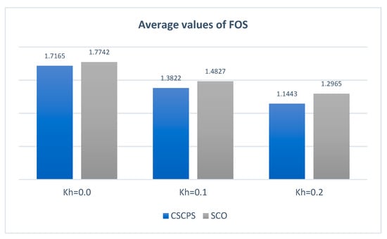
Figure 12. Average values of FOS for slope in a uniform soil.

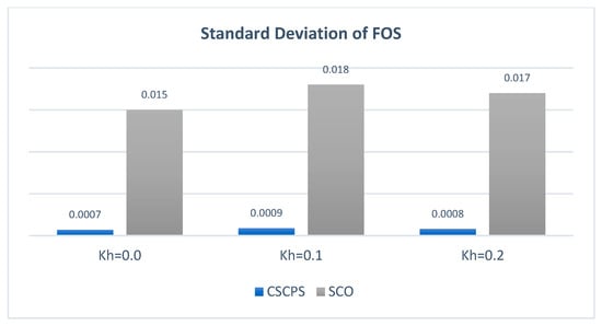
Figure 13. Standard deviation of FOS for slope in a uniform soil.

In addition, for a slope in a multi-layered soil, the FOS mean and standard deviation from 30 separate runs for various load conditions are shown in Figure 14 and Figure 15. According to these figures, the mean and standard deviation of the results obtained by CSCPS are lower than those obtained by SCO. Based on the above findings, it can be inferred that the novel CSCPS can be used to successfully evaluate the seismic stability of a multi-layered soil slope in the presence of groundwater.

Figure 14. Average values of FOS for multi-layered soil slope.

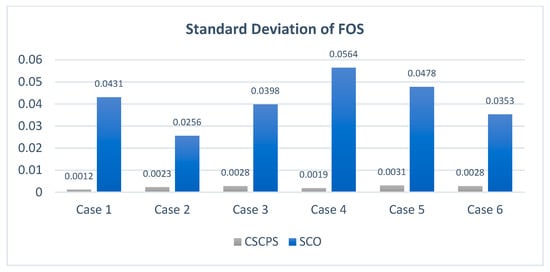
Figure 15. Standard deviation of FOS for multi-layered soil slope.

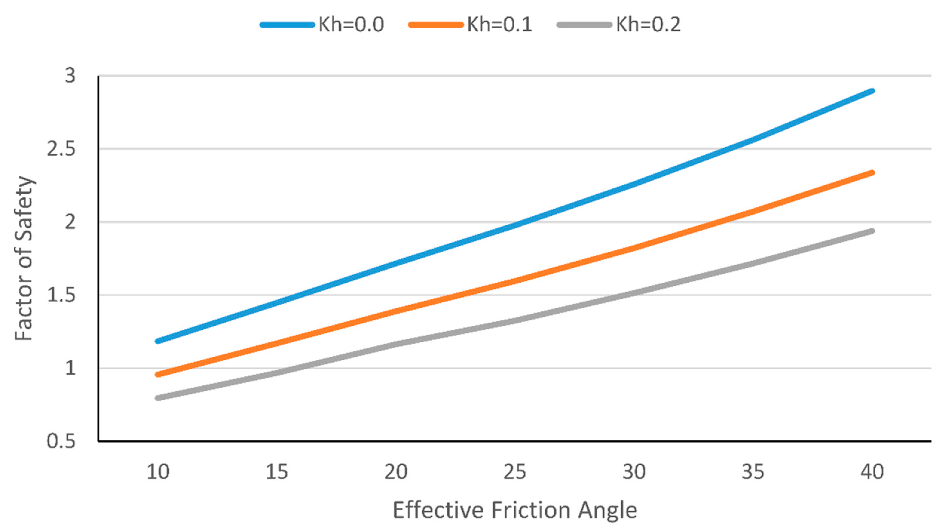
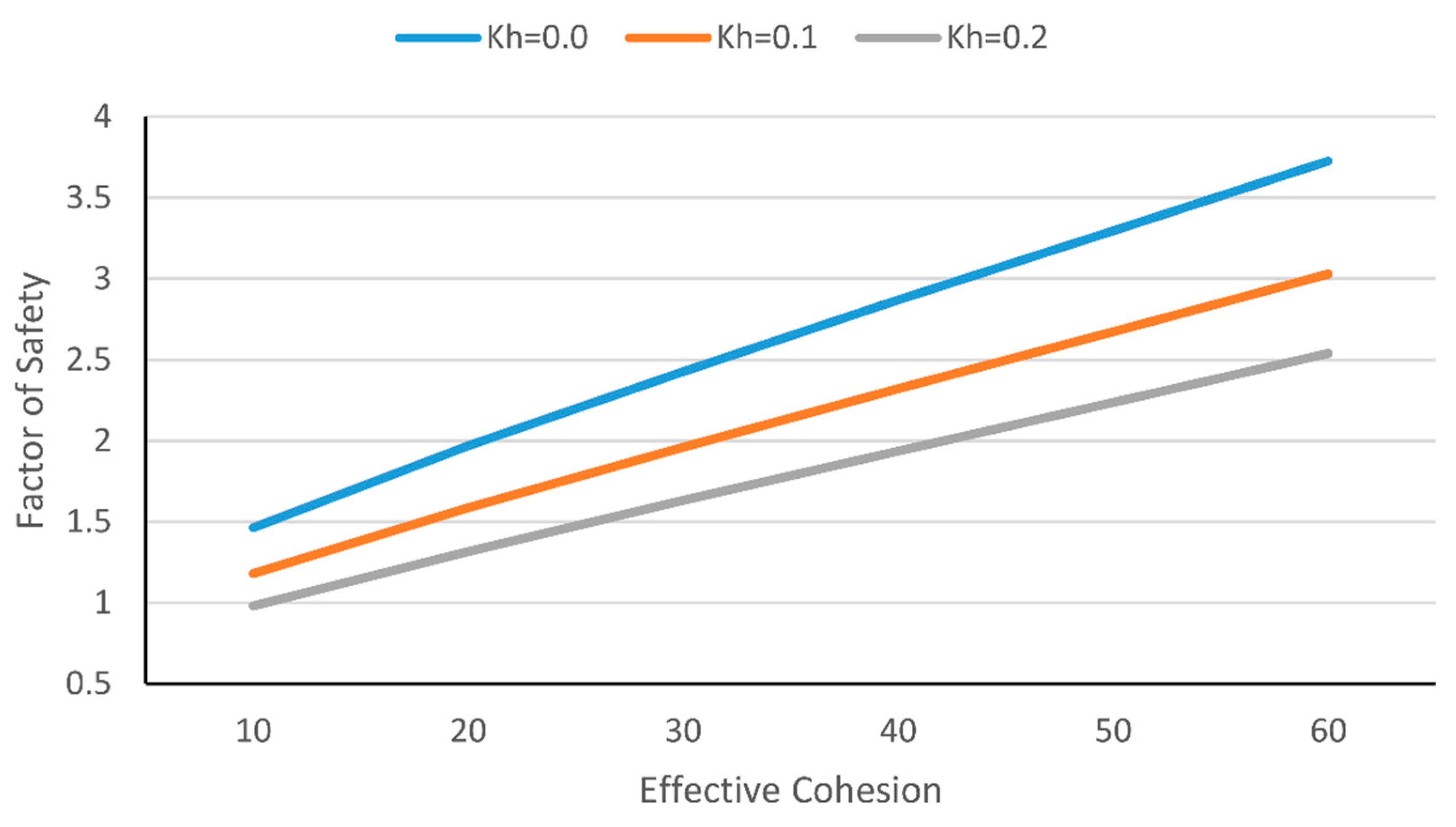
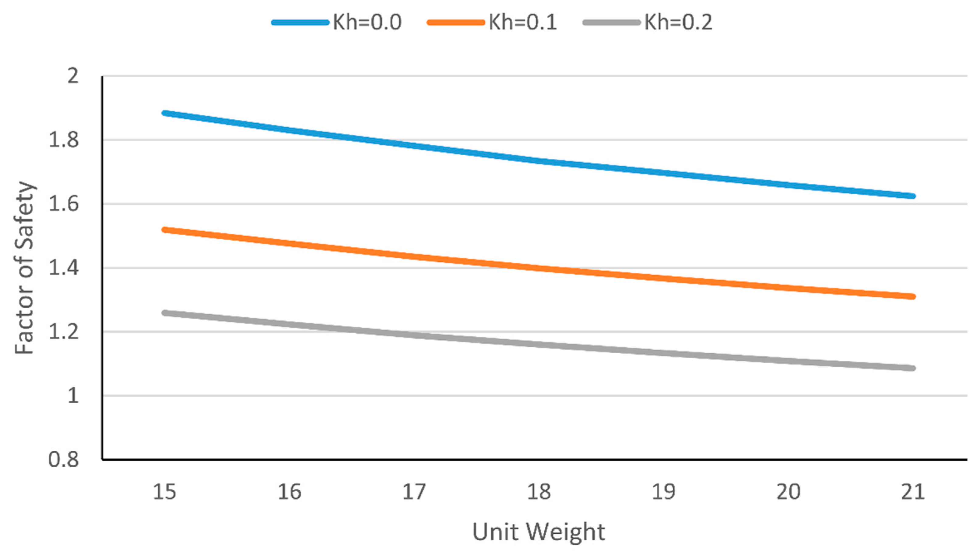
In addition, in this section, we recount how a sensitivity analysis was carried out by using the proposed methodology in order to determine the impact of the horizontal acceleration coefficient and soil characteristics, such as effective friction angle, effective cohesion, and unit weight, on the minimum factor of safety (FOS) for earth slopes. To this aim, the first case study presented in Section 5.1 underwent a sensitivity assessment. The results of the analysis are displayed graphically in Figure 16, Figure 17 and Figure 18.

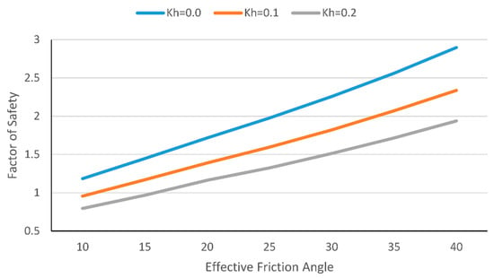
Figure 16. Effect of K_h and effective friction angle on FOS.

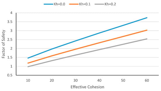
Figure 17. Effect of K_h and effective cohesion on FOS.

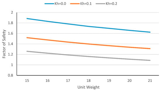
Figure 18. Effect of K_h and unit weight on FOS.

Figure 16, Figure 17 and Figure 18 depict the minimum FOS for various values of K_h (i.e., K_h = 0.0, K_h = 0.1, and K_h = 0.2) when the soil’s friction angle, cohesion, and unit weight all change within their reasonable boundaries. As seen in Figure 16 and Figure 17, as the soil’s friction angle and cohesion increase, the slope’s FOS will also increase. However, as presented in Figure 18, the relationship between FOS and unit weight is reversed, as expected. In addition, as illustrated in these figures, compared to K_h = 0.0, K_h = 0.1 results in an average 19% reduction in FOS. Moreover, when compared to the zero value of K_h, the decrement in FOS for K_h equal to 0.2 is almost 32 percent.

7. Conclusions

This research provides a hybrid optimization technique based on the chaotic sand cat, as well as pattern search (CSCPS), for assessing the safety of soil slopes subjected to seismic loads. The suggested methodology uses the powerful exploratory ability of the chaos sand cat optimization, as well as the efficient local search capacity of the pattern search technique. A variety of benchmark functions, both unimodal and multimodal, were used to assess the performance of the new approach. Considering the obtained results, the CSCPS outperforms the standard SCO and some other commonly used metaheuristic algorithms such as PSO, FA, MVO, SSA, and TSA. The optimization results of benchmark functions revealed that the new method could reach the global optimum for eight functions and a near-optimal solution for the others. Moreover, the standard deviations obtained by the CSCPS are significantly lower than those obtained by other methods, thus indicating the stability of the algorithm. The proposed CSCPS was then used to find the minimum safety factor and its associated critical failure surface of earth slopes in the existence of seismic loading. Two numerical experiments of single-layered and multi-layered soil slopes were considered from the literature. The findings show that the newly suggested methodology can improve the results of the prior methods (i.e., PSO and GA) by up to 10%, indicating that CSCPS is quite efficient for solving such a complex engineering problem. In future work, the proposed method will be further applied to reinforced slopes, three-dimensional slopes, and other geotechnical engineering optimization problems.

References

- Khajehzadeh, M.; Taha, M.R.; El-Shafie, A.; Eslami, M. Locating the general failure surface of earth slope using particle swarm optimization. Civ. Eng. Environ. Syst. 2012, 29, 41–57. [Google Scholar] [CrossRef]
- Chen, Z.; Shao, C. Evaluation of minimum factor of safety in slope stability analysis. Can. Geotech. J. 1988, 25, 735–748. [Google Scholar] [CrossRef]
- Aryal, K.; Sandven, R.; Nordal, S. Slope stability evaluation by limit equilibrium and finite element methods. In Proceedings of the 16th International Conference on Soil Mechanics and Geotechnical Engineering, Osaka, Japan, 12–16 September 2005; pp. 2471–2476. [Google Scholar]
- Baker, R.; Shukha, R.; Operstein, V.; Frydman, S. Stability charts for pseudo-static slope stability analysis. Soil Dyn. Earthq. Eng. 2006, 26, 813–823. [Google Scholar] [CrossRef]
- Tang, H.; Liu, X.; Xiong, C.; Wang, Z.; Ez Eldin, M. Proof of nondeterministic polynomial-time complete problem for soil slope-stability evaluation. Int. J. Geomech. 2016, 16, C4015004. [Google Scholar] [CrossRef]
- Zolfaghari, A.R.; Heath, A.C.; McCombie, P.F. Simple genetic algorithm search for critical non-circular failure surface in slope stability analysis. Comput. Geotech. 2005, 32, 139–152. [Google Scholar] [CrossRef]
- Wang, H.; Moayedi, H.; Kok Foong, L. Genetic algorithm hybridized with multilayer perceptron to have an economical slope stability design. Eng. Comput. 2021, 37, 3067–3078. [Google Scholar] [CrossRef]
- Cheng, Y.; Li, L.; Chi, S. Performance studies on six heuristic global optimization methods in the location of critical slip surface. Comput. Geotech. 2007, 34, 462–484. [Google Scholar] [CrossRef]
- Kashani, A.R.; Gandomi, A.H.; Mousavi, M. Imperialistic competitive algorithm: A metaheuristic algorithm for locating the critical slip surface in 2-dimensional soil slopes. Geosci. Front. 2016, 7, 83–89. [Google Scholar] [CrossRef] [Green Version]
- Gandomi, A.; Kashani, A.; Mousavi, M.; Jalalvandi, M. Slope stability analysis using evolutionary optimization techniques. Int. J. Numer. Anal. Methods Geomech. 2017, 41, 251–264. [Google Scholar] [CrossRef]
- Himanshu, N.; Burman, A. Determination of critical failure surface of slopes using particle swarm optimization technique considering seepage and seismic loading. Geotech. Geol. Eng. 2019, 37, 1261–1281. [Google Scholar] [CrossRef]
- Khajehzadeh, M.; Taha, M.; El-Shafie, A. Reliability analysis of earth slopes using hybrid chaotic particle swarm optimization. J. Cent. South Univ. Technol. 2011, 18, 1626–1637. [Google Scholar] [CrossRef]
- Eslami, M.; Shareef, H.; Mohamed, A.; Khajehzadeh, M. Optimal location of PSS using improved PSO with chaotic sequence. In Proceedings of the International Conference on Electrical, Control and Computer Engineering 2011 (InECCE), Kuantan, Malaysia, 21–22 June 2011; pp. 253–258. [Google Scholar]
- Delice, Y.; Aydoğan, E.K.; Özcan, U.; İlkay, M.S. A modified particle swarm optimization algorithm to mixed-model two-sided assembly line balancing. J. Intell. Manuf. 2017, 28, 23–36. [Google Scholar] [CrossRef]
- Eslami, M.; Shareef, H.; Mohamed, A. Optimization and coordination of damping controls for optimal oscillations damping in multi-machine power system. Int. Rev. Electr. Eng. 2011, 6, 1984–1993. [Google Scholar]
- Cheng, Y.; Li, L.; Lansivaara, T.; Chi, S.; Sun, Y. An improved harmony search minimization algorithm using different slip surface generation methods for slope stability analysis. Eng. Optim. 2008, 40, 95–115. [Google Scholar] [CrossRef]
- Khajehzadeh, M.; Taha, M.R.; Eslami, M. Multi-objective optimisation of retaining walls using hybrid adaptive gravitational search algorithm. Civ. Eng. Environ. Syst. 2014, 31, 229–242. [Google Scholar] [CrossRef]
- Ji, Y.; Tu, J.; Zhou, H.; Gui, W.; Liang, G.; Chen, H.; Wang, M. An adaptive chaotic sine cosine algorithm for constrained and unconstrained optimization. Complexity 2020, 2020, 6084917. [Google Scholar] [CrossRef]
- Hegazy, A.E.; Makhlouf, M.; El-Tawel, G.S. Improved salp swarm algorithm for feature selection. J. King Saud Univ.-Comput. Inf. Sci. 2020, 32, 335–344. [Google Scholar] [CrossRef]
- Gao, W. Modified ant colony optimization with improved tour construction and pheromone updating strategies for traveling salesman problem. Soft Comput. 2021, 25, 3263–3289. [Google Scholar] [CrossRef]
- Duan, D.; Poursoleiman, R. Modified teaching-learning-based optimization by orthogonal learning for optimal design of an electric vehicle charging station. Util. Policy 2021, 72, 101253. [Google Scholar] [CrossRef]
- Li, L.-L.; Liu, Z.-F.; Tseng, M.-L.; Zheng, S.-J.; Lim, M.K. Improved tunicate swarm algorithm: Solving the dynamic economic emission dispatch problems. Appl. Soft Comput. 2021, 108, 107504. [Google Scholar] [CrossRef]
- Ali, M.H.; Kamel, S.; Hassan, M.H.; Tostado-Véliz, M.; Zawbaa, H.M. An improved wild horse optimization algorithm for reliability based optimal DG planning of radial distribution networks. Energy Rep. 2022, 8, 582–604. [Google Scholar] [CrossRef]
- Qi, C.; Tang, X. Slope stability prediction using integrated metaheuristic and machine learning approaches: A comparative study. Comput. Ind. Eng. 2018, 118, 112–122. [Google Scholar] [CrossRef]
- Azarafza, M.; Akgün, H.; Ghazifard, A.; Asghari-Kaljahi, E.; Rahnamarad, J.; Derakhshani, R. Discontinuous rock slope stability analysis by limit equilibrium approaches—A review. Int. J. Digit. Earth 2021, 14, 1918–1941. [Google Scholar] [CrossRef]
- Azarafza, M.; Akgün, H.; Feizi-Derakhshi, M.-R.; Azarafza, M.; Rahnamarad, J.; Derakhshani, R. Discontinuous rock slope stability analysis under blocky structural sliding by fuzzy key-block analysis method. Heliyon 2020, 6, e03907. [Google Scholar] [CrossRef] [PubMed]
- Azarafza, M.; Akgün, H.; Ghazifard, A.; Asghari-Kaljahi, E. Key-block based analytical stability method for discontinuous rock slope subjected to toppling failure. Comput. Geotech. 2020, 124, 103620. [Google Scholar] [CrossRef]
- Goh, A. Search for critical slip circle using genetic algorithms. Civ. Eng. Environ. Syst. 2000, 17, 181–211. [Google Scholar] [CrossRef]
- Cheng, Y.M.; Li, L.; Chi, S.-C.; Wei, W. Particle swarm optimization algorithm for the location of the critical non-circular failure surface in two-dimensional slope stability analysis. Comput. Geotech. 2007, 34, 92–103. [Google Scholar] [CrossRef]
- Chan, C.M.; Zhang, L.; Ng, J.T. Optimization of pile groups using hybrid genetic algorithms. J. Geotech. Geoenviron. Eng. 2009, 135, 497–505. [Google Scholar] [CrossRef]
- Kahatadeniya, K.S.; Nanakorn, P.; Neaupane, K.M. Determination of the critical failure surface for slope stability analysis using ant colony optimization. Eng. Geol. 2009, 108, 133–141. [Google Scholar] [CrossRef]
- Khajehzadeh, M.; Taha, M.R.; El-Shafie, A.; Eslami, M. Modified particle swarm optimization for optimum design of spread footing and retaining wall. J. Zhejiang Univ.-Sci. A 2011, 12, 415–427. [Google Scholar] [CrossRef]
- Camp, C.V.; Akin, A. Design of retaining walls using big bang–big crunch optimization. J. Struct. Eng. 2012, 138, 438–448. [Google Scholar] [CrossRef]
- Camp, C.V.; Assadollahi, A. CO2 and cost optimization of reinforced concrete footings using a hybrid big bang-big crunch algorithm. Struct. Multidiscip. Optim. 2013, 48, 411–426. [Google Scholar] [CrossRef]
- Khajehzadeh, M.; Taha, M.R.; Eslami, M. A new hybrid firefly algorithm for foundation optimization. Natl. Acad. Sci. Lett. 2013, 36, 279–288. [Google Scholar] [CrossRef]
- Kang, F.; Li, J.; Ma, Z. An artificial bee colony algorithm for locating the critical slip surface in slope stability analysis. Eng. Optim. 2013, 45, 207–223. [Google Scholar] [CrossRef]
- Khajehzadeh, M.; Taha, M.R.; Eslami, M. Multi-objective optimization of foundation using global-local gravitational search algorithm. Struct. Eng. Mech. Int. J. 2014, 50, 257–273. [Google Scholar] [CrossRef]
- Gordan, B.; Jahed Armaghani, D.; Hajihassani, M.; Monjezi, M. Prediction of seismic slope stability through combination of particle swarm optimization and neural network. Eng. Comput. 2016, 32, 85–97. [Google Scholar] [CrossRef]
- Gandomi, A.H.; Kashani, A.R. Construction cost minimization of shallow foundation using recent swarm intelligence techniques. IEEE Trans. Ind. Inform. 2017, 14, 1099–1106. [Google Scholar] [CrossRef]
- Aydogdu, I. Cost optimization of reinforced concrete cantilever retaining walls under seismic loading using a biogeography-based optimization algorithm with Levy flights. Eng. Optim. 2017, 49, 381–400. [Google Scholar] [CrossRef]
- Mahdiyar, A.; Hasanipanah, M.; Armaghani, D.J.; Gordan, B.; Abdullah, A.; Arab, H.; Majid, M.Z.A. A Monte Carlo technique in safety assessment of slope under seismic condition. Eng. Comput. 2017, 33, 807–817. [Google Scholar] [CrossRef]
- Gandomi, A.; Kashani, A.; Zeighami, F. Retaining wall optimization using interior search algorithm with different bound constraint handling. Int. J. Numer. Anal. Methods Geomech. 2017, 41, 1304–1331. [Google Scholar] [CrossRef]
- Chen, H.; Asteris, P.G.; Jahed Armaghani, D.; Gordan, B.; Pham, B.T. Assessing dynamic conditions of the retaining wall: Developing two hybrid intelligent models. Appl. Sci. 2019, 9, 1042. [Google Scholar] [CrossRef] [Green Version]
- Koopialipoor, M.; Jahed Armaghani, D.; Hedayat, A.; Marto, A.; Gordan, B. Applying various hybrid intelligent systems to evaluate and predict slope stability under static and dynamic conditions. Soft Comput. 2019, 23, 5913–5929. [Google Scholar] [CrossRef]
- Yang, H.; Koopialipoor, M.; Armaghani, D.J.; Gordan, B.; Khorami, M.; Tahir, M. Intelligent design of retaining wall structures under dynamic conditions. Steel Compos. Struct. Int. J. 2019, 31, 629–640. [Google Scholar]
- Xu, C.; Gordan, B.; Koopialipoor, M.; Armaghani, D.J.; Tahir, M.; Zhang, X. Improving performance of retaining walls under dynamic conditions developing an optimized ANN based on ant colony optimization technique. IEEE Access 2019, 7, 94692–94700. [Google Scholar] [CrossRef]
- Kalemci, E.N.; İkizler, S.B.; Dede, T.; Angın, Z. Design of reinforced concrete cantilever retaining wall using Grey wolf optimization algorithm. Structures 2020, 23, 245–253. [Google Scholar] [CrossRef]
- Kaveh, A.; Hamedani, K.B.; Bakhshpoori, T. Optimal design of reinforced concrete cantilever retaining walls utilizing eleven meta-heuristic algorithms: A comparative study. Period Polytech. Civ. Eng. 2020, 64, 156–168. [Google Scholar] [CrossRef]
- Kashani, A.R.; Gandomi, M.; Camp, C.V.; Gandomi, A.H. Optimum design of shallow foundation using evolutionary algorithms. Soft Comput. 2020, 24, 6809–6833. [Google Scholar] [CrossRef]
- Wang, L.; Wu, C.; Tang, L.; Zhang, W.; Lacasse, S.; Liu, H.; Gao, L. Efficient reliability analysis of earth dam slope stability using extreme gradient boosting method. Acta Geotech. 2020, 15, 3135–3150. [Google Scholar] [CrossRef]
- Moayedi, H.; Osouli, A.; Nguyen, H.; Rashid, A.S.A. A novel Harris hawks’ optimization and k-fold cross-validation predicting slope stability. Eng. Comput. 2021, 37, 369–379. [Google Scholar] [CrossRef]
- Sharma, S.; Saha, A.K.; Lohar, G. Optimization of weight and cost of cantilever retaining wall by a hybrid metaheuristic algorithm. Eng. Comput. 2021, 1–27. [Google Scholar] [CrossRef]
- Kaveh, A.; Seddighian, M.R. Optimization of Slope Critical Surfaces Considering Seepage and Seismic Effects Using Finite Element Method and Five Meta-Heuristic Algorithms. Period. Polytech. Civ. Eng. 2021, 65, 425–436. [Google Scholar] [CrossRef]
- Temur, R. Optimum design of cantilever retaining walls under seismic loads using a hybrid TLBO algorithm. Geomech. Eng. 2021, 24, 237–251. [Google Scholar]
- Li, S.; Wu, L. An improved salp swarm algorithm for locating critical slip surface of slopes. Arab. J. Geosci. 2021, 14, 1–11. [Google Scholar] [CrossRef]
- Arabali, A.; Khajehzadeh, M.; Keawsawasvong, S.; Mohammed, A.H.; Khan, B. An Adaptive Tunicate Swarm Algorithm for Optimization of Shallow Foundation. IEEE Access 2022, 10, 39204–39219. [Google Scholar] [CrossRef]
- Khajehzadeh, M.; Keawsawasvong, S.; Nehdi, M.L. Effective hybrid soft computing approach for optimum design of shallow foundations. Sustainability 2022, 14, 1847. [Google Scholar] [CrossRef]
- Khajehzadeh, M.; Kalhor, A.; Tehrani, M.S.; Jebeli, M. Optimum design of retaining structures under seismic loading using adaptive sperm swarm optimization. Struct. Eng. Mech. 2022, 81, 93–102. [Google Scholar]
- Kashani, A.R.; Camp, C.V.; Azizi, K.; Rostamian, M. Multi-objective optimization of mechanically stabilized earth retaining wall using evolutionary algorithms. Int. J. Numer. Anal. Methods Geomech. 2022, 46, 3352. [Google Scholar] [CrossRef]
- Seyyedabbasi, A.; Kiani, F. Sand Cat swarm optimization: A nature-inspired algorithm to solve global optimization problems. Eng. Comput. 2022, 1–25. [Google Scholar] [CrossRef]
- Dolan, E.D.; Lewis, R.M.; Torczon, V. On the local convergence of pattern search. SIAM J. Optim. 2003, 14, 567–583. [Google Scholar] [CrossRef]
- Duncan, J.M. State of the art: Limit equilibrium and finite-element analysis of slopes. J. Geotech. Eng. 1996, 122, 577–596. [Google Scholar] [CrossRef]
- Morgenstern, N.R.; Price, V.E. The analysis of the stability of general slip surfaces. Geotechinque 1965, 15, 79–93. [Google Scholar] [CrossRef]
- Zhu, D.; Lee, C.; Qian, Q.; Chen, G. A concise algorithm for computing the factor of safety using the Morgenstern–Price method. Can. Geotech. J. 2005, 42, 272–278. [Google Scholar] [CrossRef] [Green Version]
- Cheng, Y. Location of critical failure surface and some further studies on slope stability analysis. Comput. Geotech. 2003, 30, 255–267. [Google Scholar] [CrossRef]
- Huang, G.; Rosowski, J.; Ravicz, M.; Peake, W. Mammalian ear specializations in arid habitats: Structural and functional evidence from sand cat (Felis margarita). J. Comp. Physiol. A 2002, 188, 663–681. [Google Scholar]
- Torczon, V. On the convergence of pattern search algorithms. SIAM J. Optim. 1997, 7, 1–25. [Google Scholar] [CrossRef]
- Cherki, I.; Chaker, A.; Djidar, Z.; Khalfallah, N.; Benzergua, F. A Sequential Hybridization of Genetic Algorithm and Particle Swarm Optimization for the Optimal Reactive Power Flow. Sustainability 2019, 11, 3862. [Google Scholar] [CrossRef] [Green Version]
- Zervoudakis, K.; Tsafarakis, S. A mayfly optimization algorithm. Comput. Ind. Eng. 2020, 145, 106559. [Google Scholar] [CrossRef]
- Kaur, S.; Awasthi, L.K.; Sangal, A.; Dhiman, G. Tunicate swarm algorithm: A new bio-inspired based metaheuristic paradigm for global optimization. Eng. Appl. Artif. Intell. 2020, 90, 103541. [Google Scholar] [CrossRef]
- Kennedy, J.; Eberhart, R. Particle swarm optimization. In Proceedings of the ICNN’95-International Conference on Neural Networks, Perth, WA, Australia, 27 November 1995; pp. 1942–1948. [Google Scholar]
- Yang, X.S. Firefly algorithms for multimodal optimization. Lect. Notes Comput. Sci. 2009, 5792, 169–178. [Google Scholar]
- Mirjalili, S.; Mirjalili, S.M.; Hatamlou, A. Multi-verse optimizer: A nature-inspired algorithm for global optimization. Neural Comput. Appl. 2016, 27, 495–513. [Google Scholar] [CrossRef]
Publisher’s Note: MDPI stays neutral with regard to jurisdictional claims in published maps and institutional affiliations. |
© 2022 by the authors. Licensee MDPI, Basel, Switzerland. This article is an open access article distributed under the terms and conditions of the Creative Commons Attribution (CC BY) license (https://creativecommons.org/licenses/by/4.0/).