
Applying PCA to Deep Learning Forecasting Models for Predicting PM2.5


Abstract
1. Introduction
2. Previous Research
3. Data
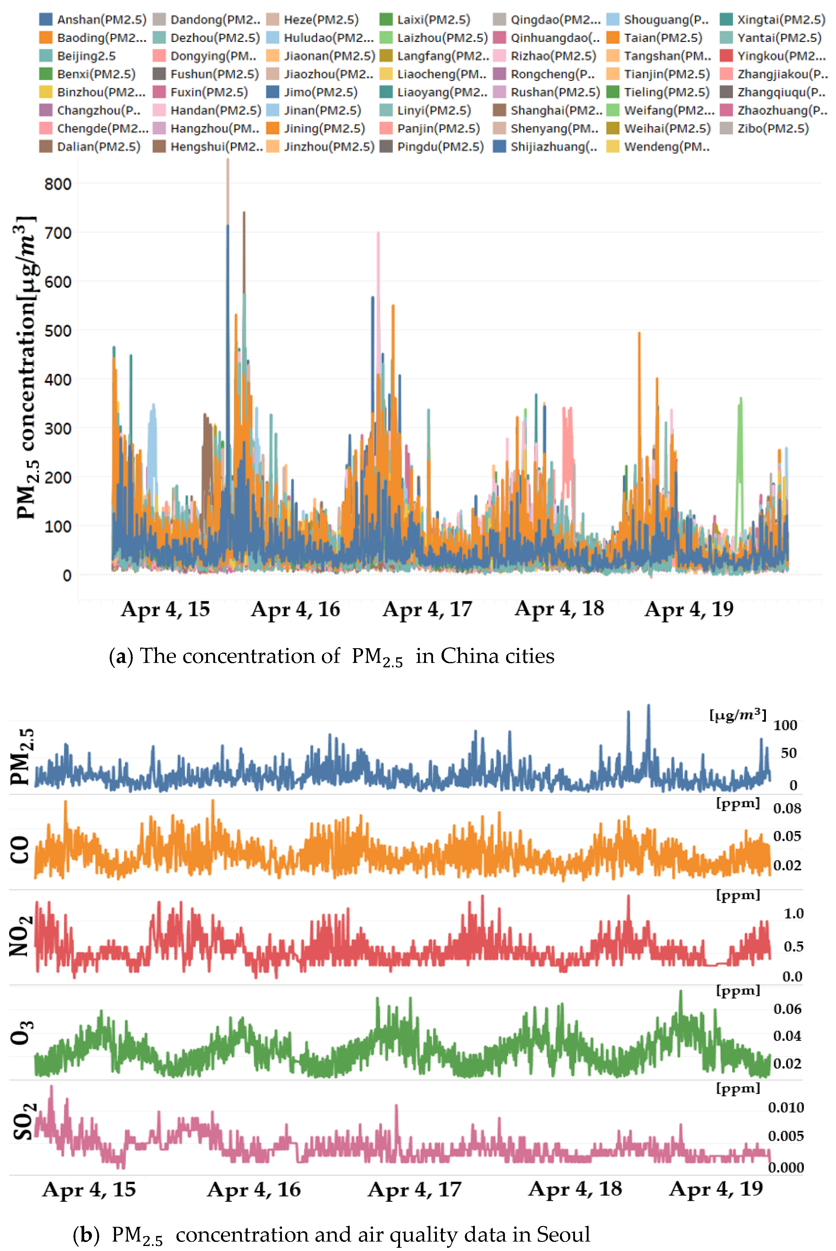
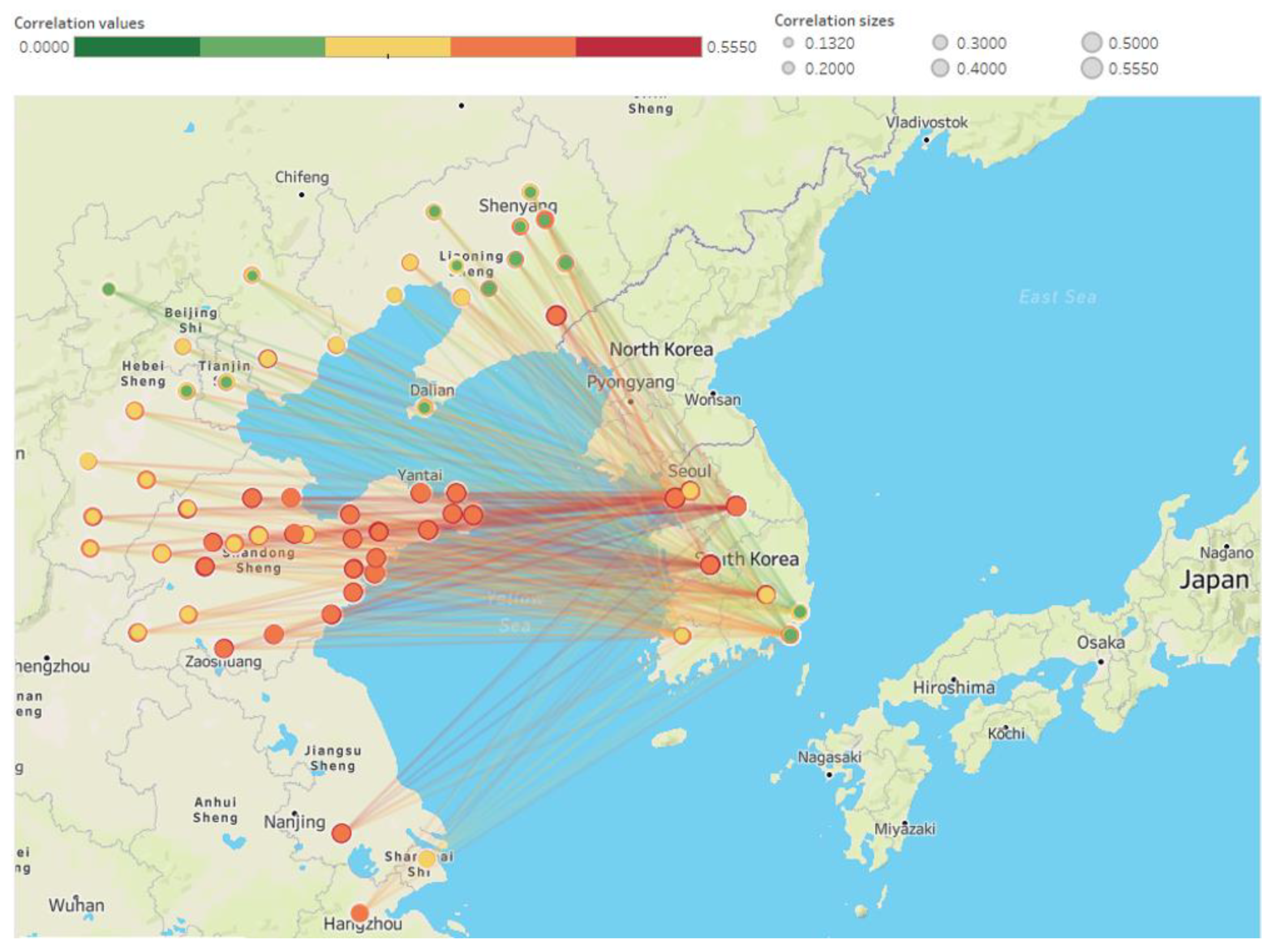
3.1. Spatial Area
3.2. Data Preprocessing
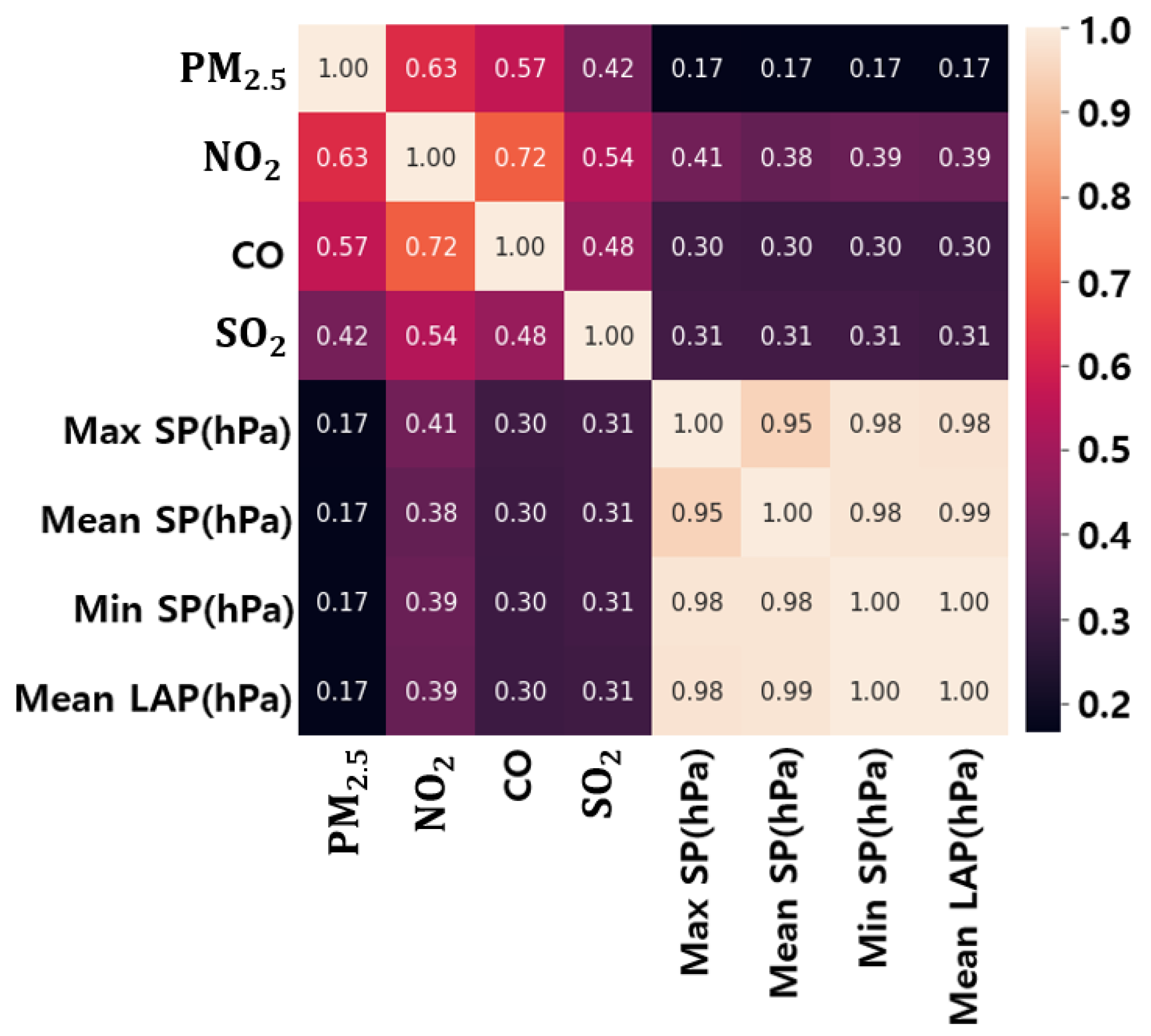
3.3. Variable Correlation Analysis
4. Analytical Methods
4.1. PCA
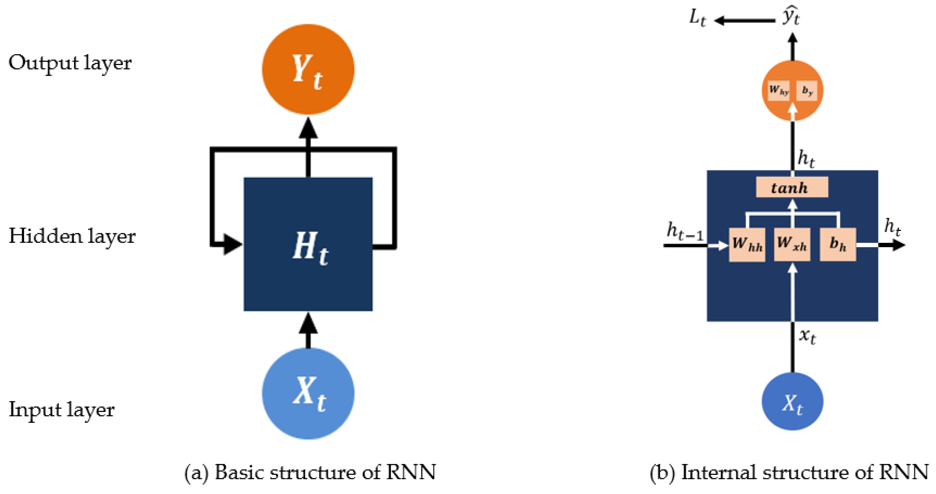
4.2. RNN
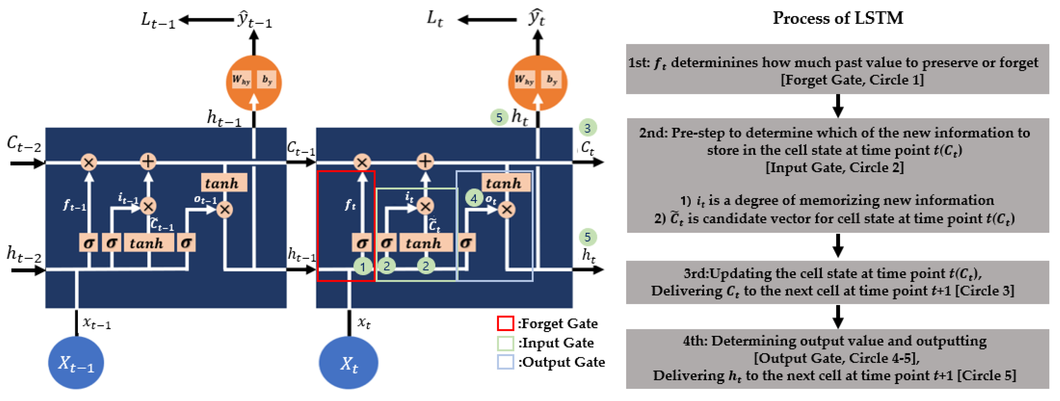
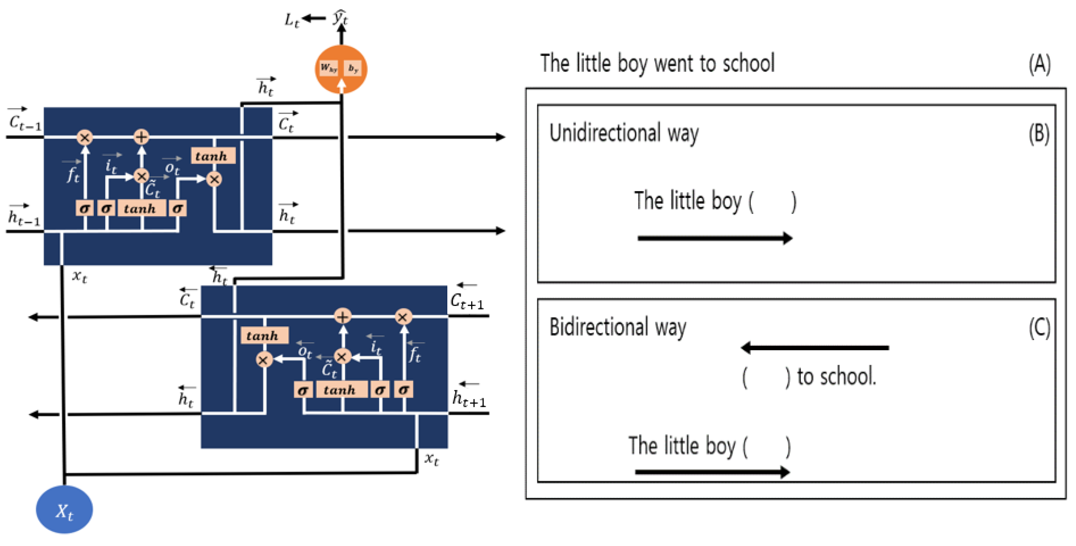
4.3. LSTM and BiLSTM
4.4. Evaluation Model Performance
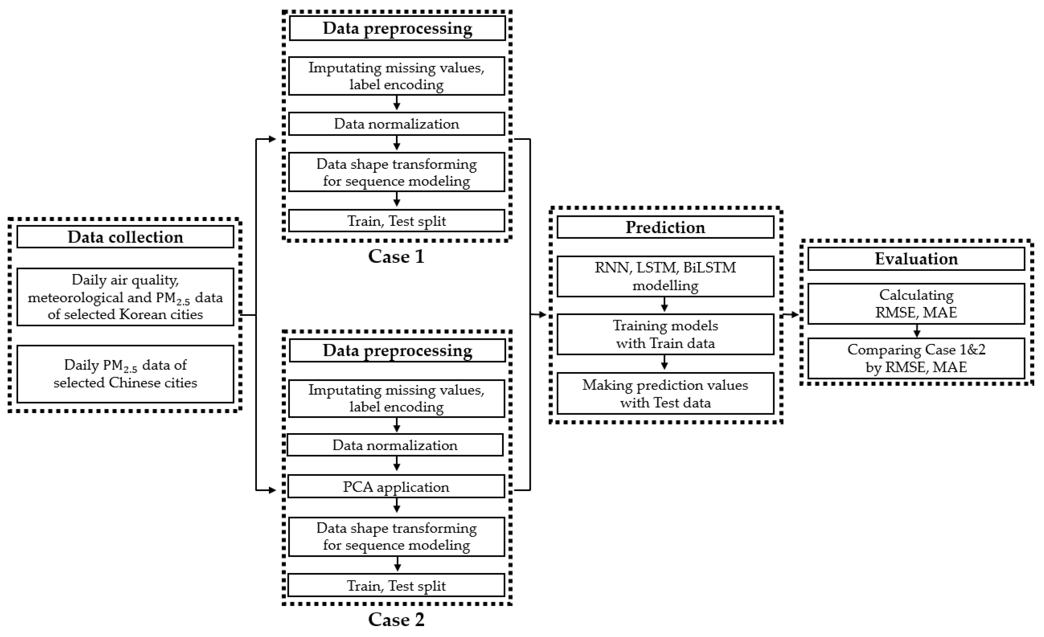
4.5. Workflow
5. Results
5.1. PC Selection
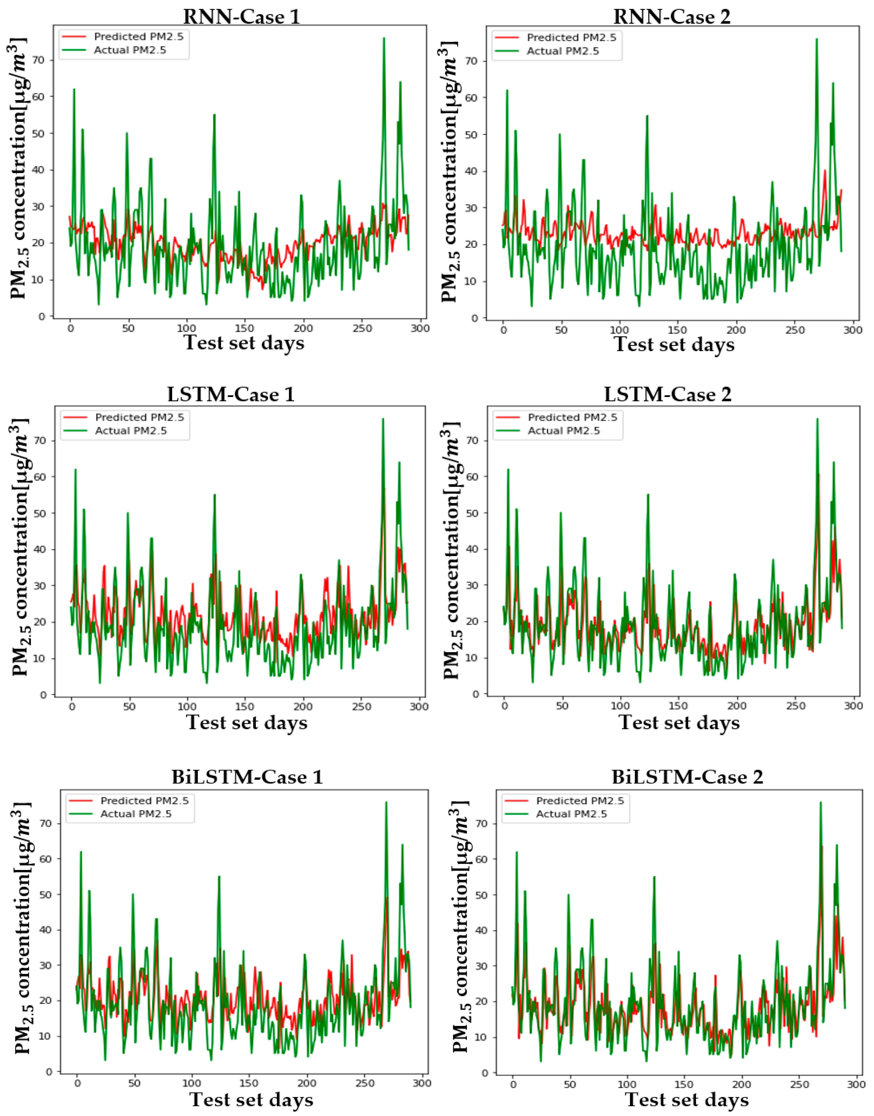
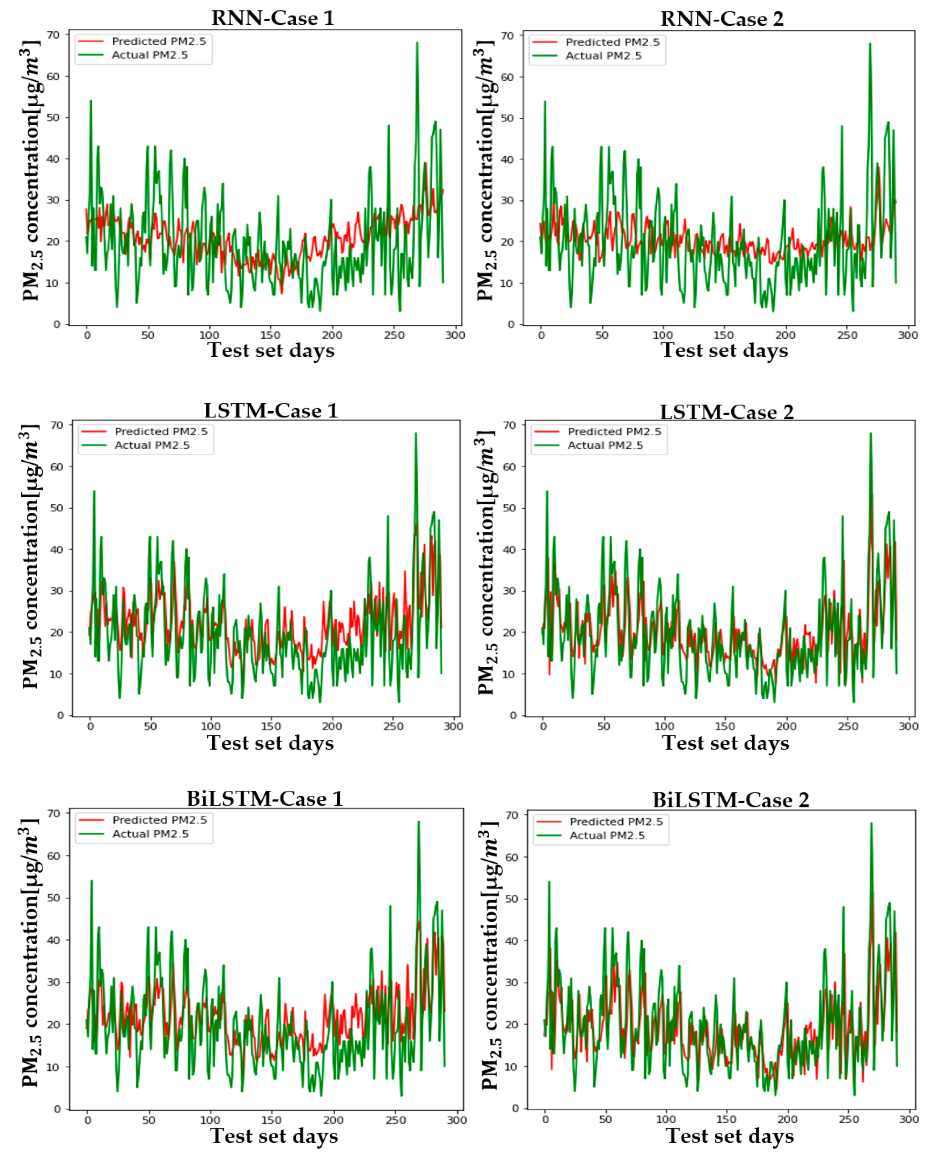
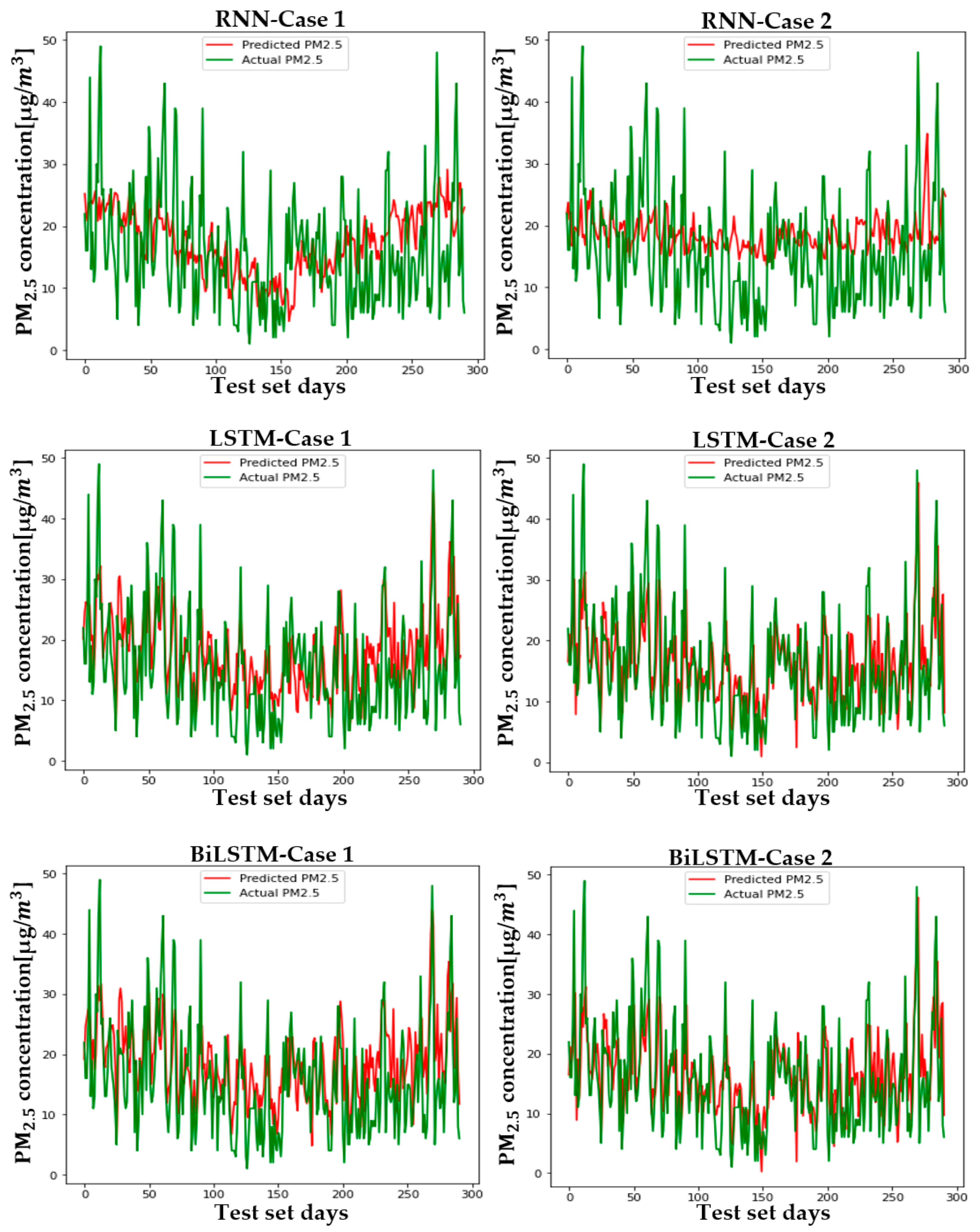
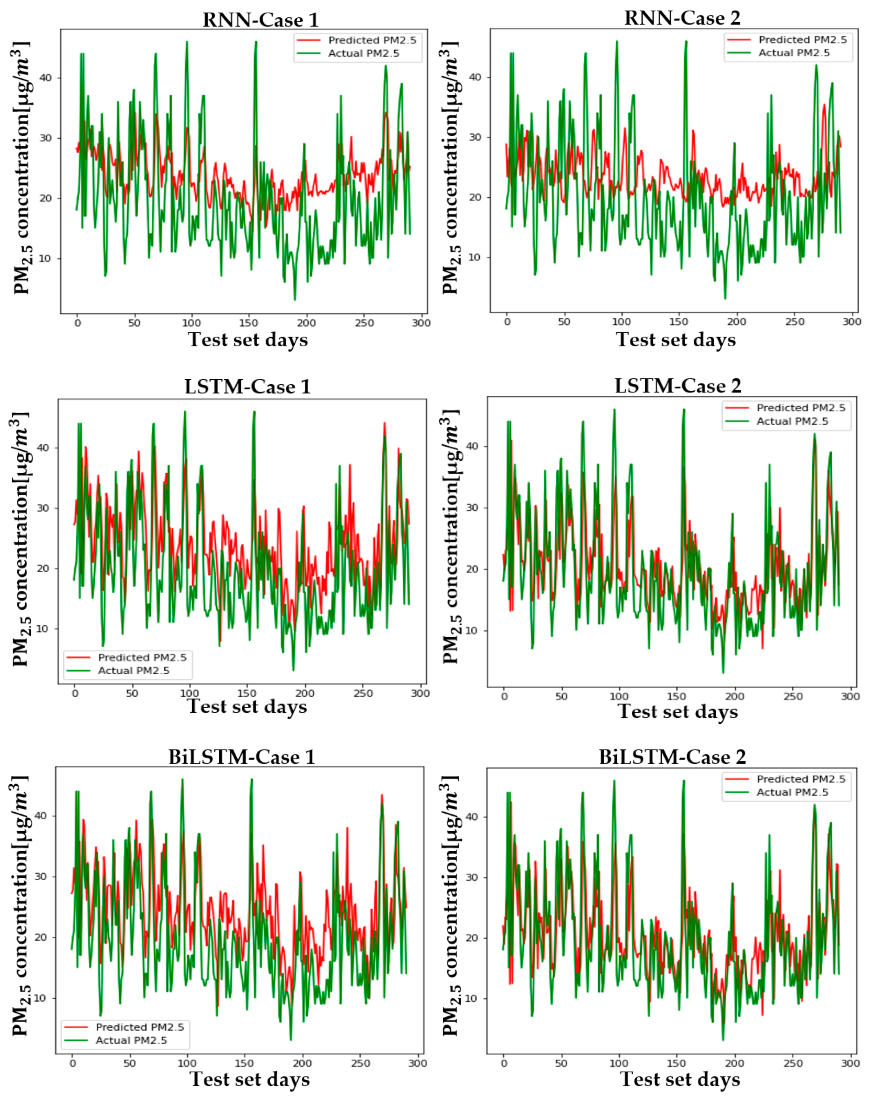
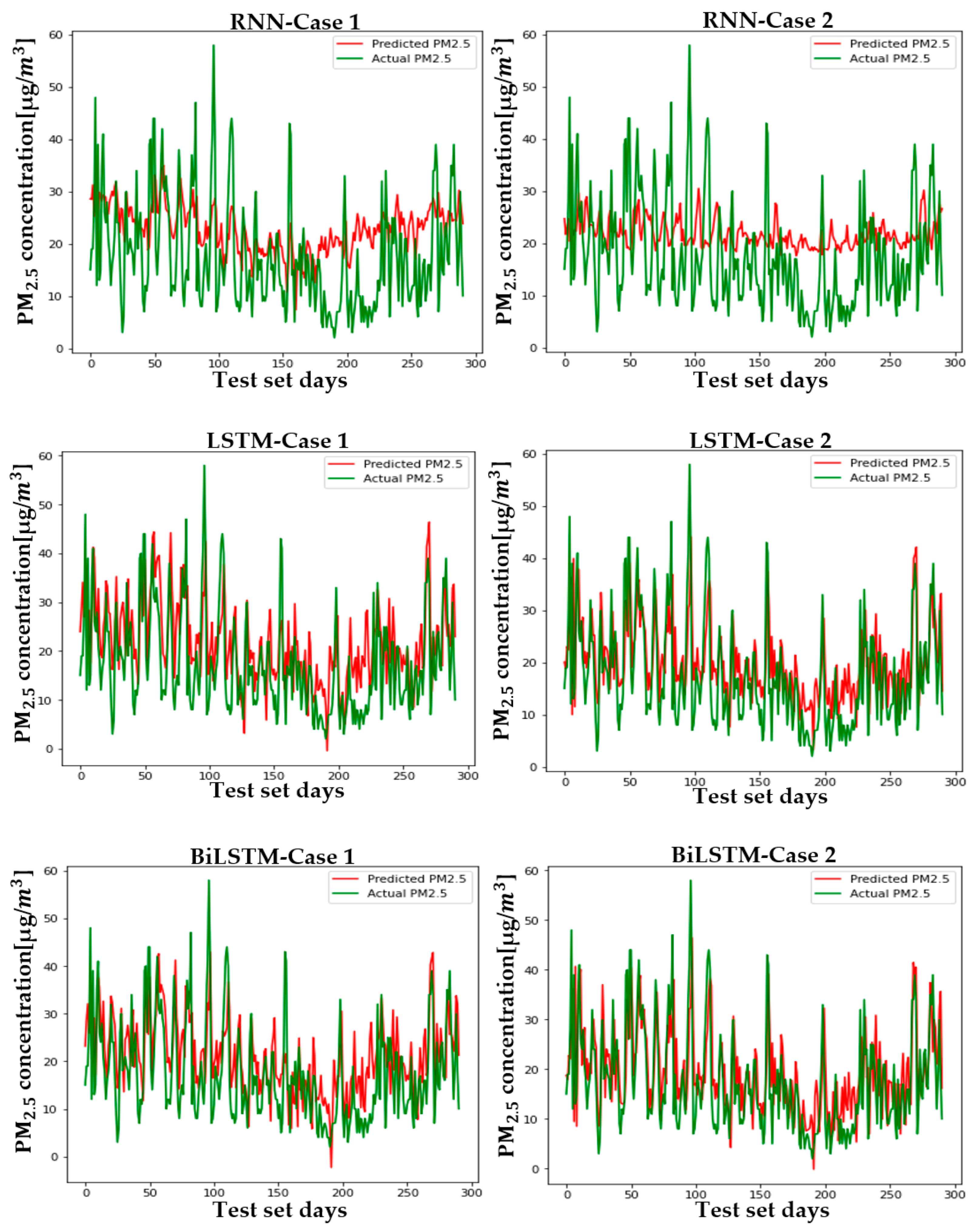
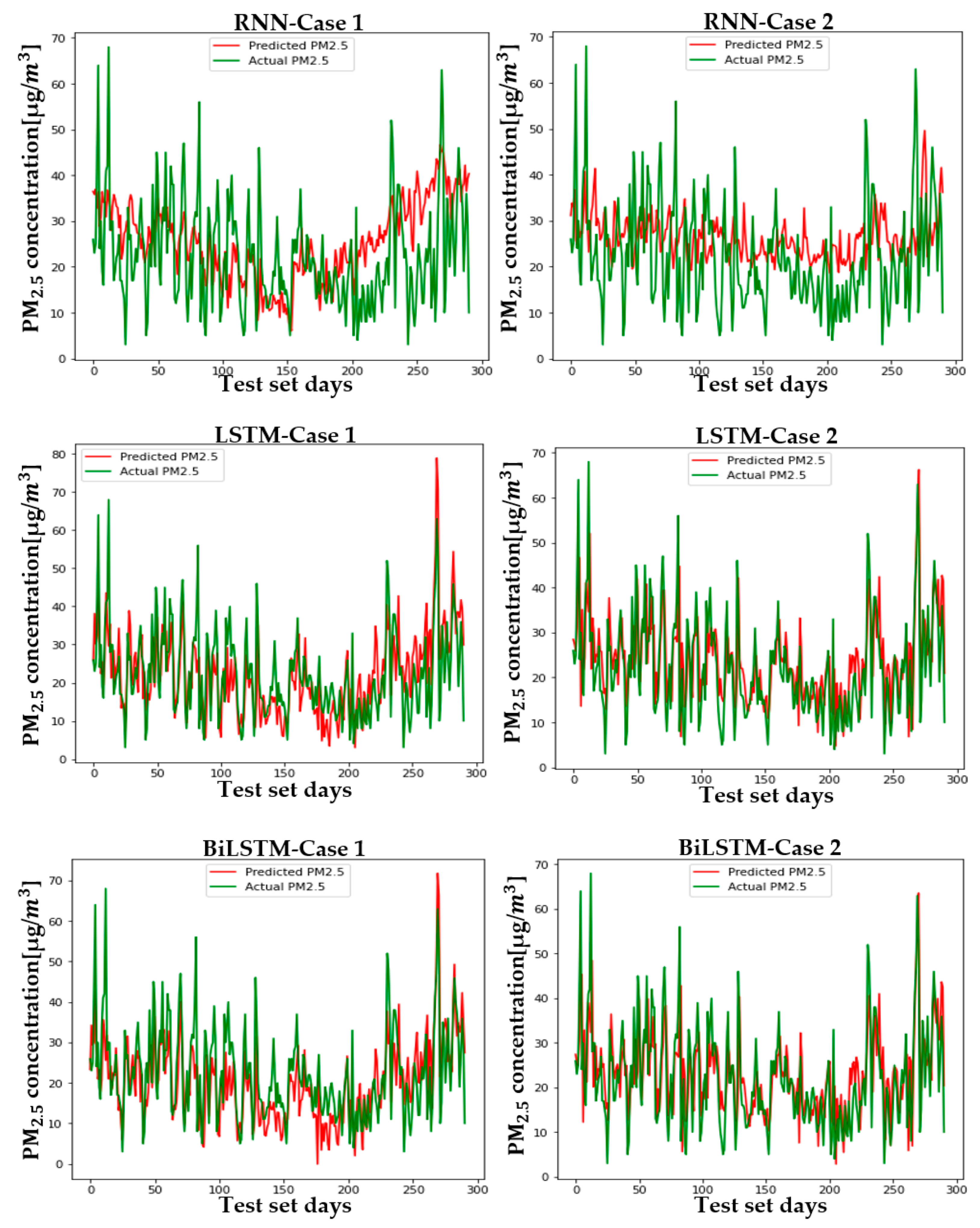
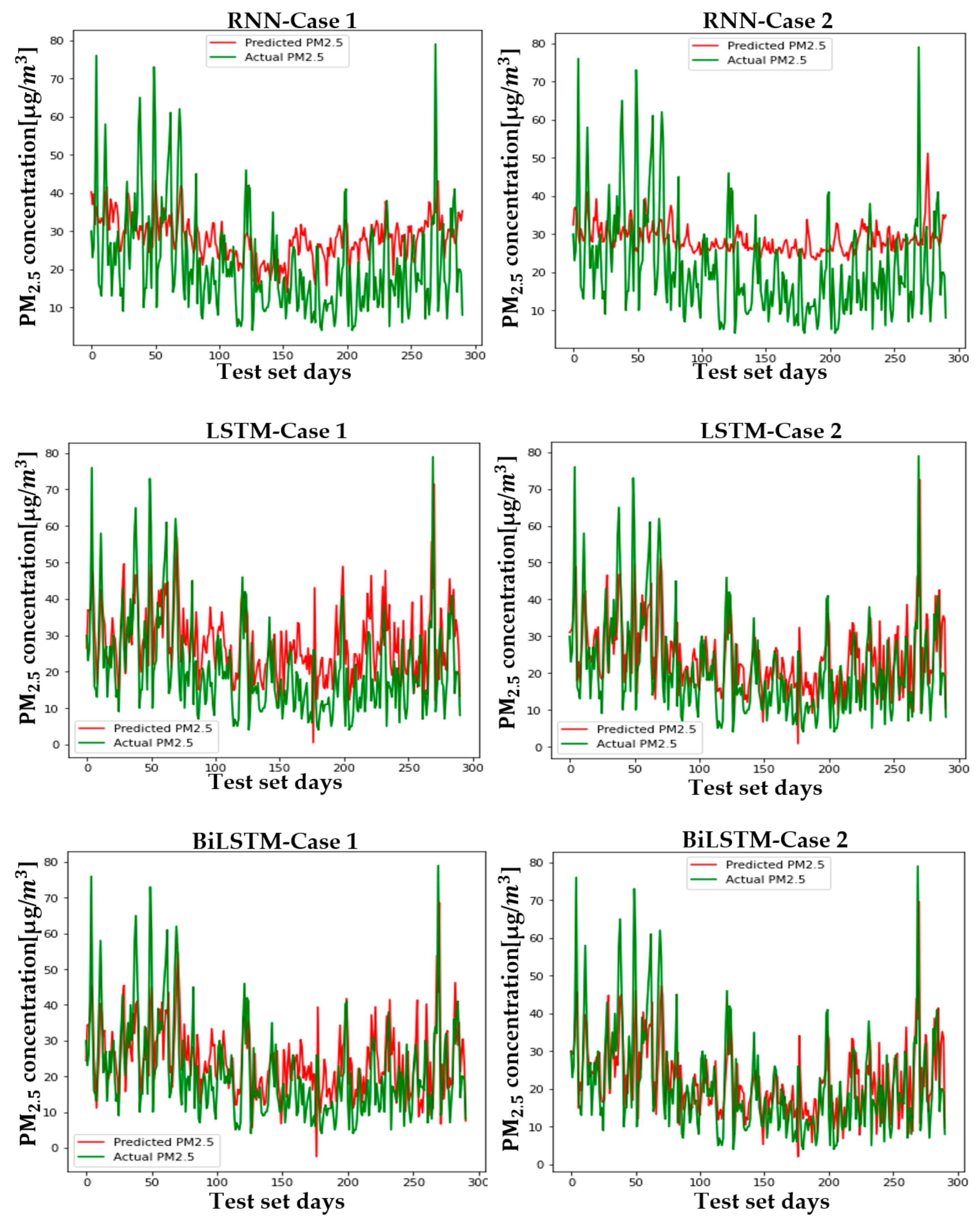
5.2. Setup and Case Comparison
6. Conclusions
Author Contributions
Funding
Institutional Review Board Statement
Informed Consent Statement
Data Availability Statement
Acknowledgments
Conflicts of Interest
Appendix A

| Acronym | Meaning |
|---|---|
| Min Temp | Minimum temperature (°C) |
| Max Temp | Maximum temperature (°C) |
| Mean Temp | Mean temperature (°C) |
| Daily prep | Daily precipitation (mm) |
| Max inst WS | Maximum instantaneous wind speed (m/s) |
| Max inst WSD | Maximum instantaneous wind speed directions (16 cardinal points) |
| Max WS | Maximum wind speed (m/s) |
| Max WSD | Maximum wind speed directions (16 cardinal points) |
| Mean WS | Mean wind speed (m/s) |
| WFS | Wind flow sum (100 m) |
| Max freq WD | Maximum frequent wind directions (16 cardinal points) |
| Mean DP | Mean dew point (°C) |
| Mean RH | Mean relative humidity (%) |
| Mean LAP | Mean local atmospheric pressure (hPa) |
| Max SP | Maximum sea-level pressure (hPa) |
| Min SP | Minimum sea-level pressure (hPa) |
| Mean SP | Mean sea-level pressure (hPa) |
| Min RH | Minimum relative humidity (%) |
| NPC | The number of principal components |
| CV | Cumulative variance |
| Air quality factors | O3 (ppm) | −0.021 | Meteorological factors | Min Temp | −0.175 | Max inst WS | −0.196 | Mean WS | −0.174 | Mean RH | 0.013 | Mean SP | 0.168 |
| CO (ppm) | 0.565 | Max Temp | −0.185 | Max inst WSD | 0.09 | WFS | −0.175 | Mean LAP | 0.166 | Min RH | −0.047 | ||
| NO2 (ppm) | 0.627 | Mean Temp | −0.156 | Max WS | −0.098 | Max freqWD | 0.041 | Max SP | 0.17 | ||||
| SO2 (ppm) | 0.417 | Daily prep | −0.143 | Max WSD | 0.118 | Mean DP | −0.141 | Min SP | 0.169 |
| Air quality factors | O3 (ppm) | 0.108 | Meteorological factors | Min Temp | −0.223 | Max inst WS | −0.226 | Mean WS | −0.28 | Mean RH | −0.164 | Mean SP | 0.192 |
| CO (ppm) | 0.532 | Max Temp | −0.122 | Max inst WSD | 0.108 | WFS | −0.281 | Mean LAP | 0.192 | Min RH | −0.235 | ||
| NO2 (ppm) | 0.562 | Mean Temp | −0.179 | Max WS | −0.214 | Max freq WD | 0.11 | Max SP | 0.186 | ||||
| SO2 (ppm) | 0.276 | Daily prep | −0.212 | Max WSD | 0.102 | Mean DP | −0.2 | Min SP | 0.196 |
| Air quality factors | O3 (ppm) | −0.113 | Meteorological factors | Min Temp | −0.291 | Max inst WS | −0.305 | Mean WS | −0.373 | Mean RH | −0.056 | Mean SP | 0.256 |
| CO (ppm) | 0.665 | Max Temp | −0.193 | Max inst WSD | 0.156 | WFS | −0.374 | Mean LAP | 0.252 | Min RH | −0.128 | ||
| NO2 (ppm) | 0.702 | Mean Temp | −0.244 | Max WS | −0.317 | Max freq WD | 0.053 | Max SP | 0.26 | ||||
| SO2 (ppm) | 0.437 | Daily prep | −0.157 | Max WSD | 0.14 | Mean DP | −0.214 | Min SP | 0.253 |
| Air quality factors | O3 (ppm) | −0.086 | Meteorological factors | Min Temp | −0.299 | Max ins tWS | −0.241 | Mean WS | −0.265 | Mean RH | −0.101 | Mean SP | 0.272 |
| CO (ppm) | 0.535 | Max Temp | −0.236 | Max inst WSD | 0.121 | WFS | −0.265 | Mean LAP | 0.271 | Min RH | −0.173 | ||
| NO2 (ppm) | 0.483 | Mean Temp | −0.272 | Max WS | −0.239 | Max freq WD | 0.211 | Max SP | 0.27 | ||||
| SO2 (ppm) | 0.41 | Daily prep | −0.18 | Max WSD | 0.1 | Mean DP | −0.271 | Min SP | 0.272 |
| Air quality factors | O3 (ppm) | 0.029 | Meteorological factors | Min Temp | −0.139 | Max inst WS | −0.231 | Mean WS | −0.162 | Mean RH | −0.126 | Mean SP | 0.104 |
| CO (ppm) | 0.32 | Max Temp | −0.095 | Max inst WSD | 0.196 | WFS | −0.162 | Mean LAP | 0.102 | Min RH | −0.187 | ||
| NO2 (ppm) | 0.554 | Mean Temp | −0.119 | Max WS | −0.07 | Max freqWD | 0.178 | Max SP | 0.086 | ||||
| SO2 (ppm) | 0.366 | Daily prep | −0.17 | Max WSD | 0.249 | Mean DP | −0.125 | Min SP | 0.124 |
| Air quality factors | O3 (ppm) | 0.095 | Meteorological factors | Min Temp | −0.084 | Max inst WS | −0.198 | Mean WS | −0.318 | Mean RH | −0.125 | Mean SP | 0.032 |
| CO (ppm) | 0.665 | Max Temp | 0.053 | Max inst WSD | 0.023 | WFS | −0.319 | Mean LAP | 0.064 | Min RH | −0.233 | ||
| NO2 (ppm) | 0.667 | Mean Temp | −0.015 | Max WS | −0.166 | Max freq WD | −0.055 | Max SP | 0.016 | ||||
| SO2 (ppm) | 0.525 | Daily prep | −0.167 | Max WSD | 0.014 | Mean DP | −0.055 | Min SP | 0.051 |
| Air quality factors | O3 (ppm) | −0.129 | Meteorological factors | Min Temp | −0.384 | Max inst WS | −0.187 | Mean WS | −0.257 | Mean RH | −0.018 | Mean SP | 0.309 |
| CO (ppm) | 0.686 | Max Temp | −0.339 | Max inst WSD | 0.171 | WFS | −0.259 | Mean LAP | 0.299 | Min RH | −0.077 | ||
| NO2 (ppm) | 0.675 | Mean Temp | −0.366 | Max WS | −0.187 | Max freq WD | 0.077 | Max SP | 0.318 | ||||
| SO2 (ppm) | 0.575 | Daily prep | −0.184 | Max WSD | 0.14 | Mean DP | −0.326 | Min SP | 0.302 |
| Air quality factors | O3 (ppm) | −0.102 | Meteorological Factors | Min Temp | −0.15 | Max inst WS | −0.288 | Mean WS | −0.308 | Mean RH | 0.214 | Mean SP | 0.149 |
| CO (ppm) | 0.621 | Max Temp | −0.122 | Max inst WSD | 0.045 | WFS | −0.309 | Mean LAP | 0.143 | Min RH | 0.091 | ||
| NO2 (ppm) | 0.667 | Mean Temp | −0.142 | Max WS | −0.254 | Max freq WD | 0.07 | Max SP | 0.155 | ||||
| SO2 (ppm) | 0.559 | Daily prep | −0.144 | Max WSD | 0.049 | Mean DP | −0.054 | Min SP | 0.151 |
| NPC | CV | NPC | CV | NPC | CV | NPC | CV | NPC | CV | NPC | CV | NPC | CV | NPC | CV |
|---|---|---|---|---|---|---|---|---|---|---|---|---|---|---|---|
| 1 | 82.06% | 11 | 97.88% | 21 | 98.99% | 31 | 99.49% | 41 | 99.77% | 51 | 99.92% | 61 | 99.99% | 71 | 100.00% |
| 2 | 93.11% | 12 | 98.04% | 22 | 99.06% | 32 | 99.52% | 42 | 99.79% | 52 | 99.93% | 62 | 100.00% | 72 | 100.00% |
| 3 | 94.58% | 13 | 98.19% | 23 | 99.12% | 33 | 99.56% | 43 | 99.81% | 53 | 99.94% | 63 | 100.00% | 73 | 100.00% |
| 4 | 95.71% | 14 | 98.33% | 24 | 99.18% | 34 | 99.59% | 44 | 99.82% | 54 | 99.95% | 64 | 100.00% | 74 | 100.00% |
| 5 | 96.31% | 15 | 98.45% | 25 | 99.23% | 35 | 99.62% | 45 | 99.84% | 55 | 99.96% | 65 | 100.00% | 75 | 100.00% |
| 6 | 96.69% | 16 | 98.56% | 26 | 99.28% | 36 | 99.65% | 46 | 99.85% | 56 | 99.97% | 66 | 100.00% | 76 | 100.00% |
| 7 | 97.01% | 17 | 98.66% | 27 | 99.33% | 37 | 99.68% | 47 | 99.87% | 57 | 99.98% | 67 | 100.00% | 77 | 100.00% |
| 8 | 97.28% | 18 | 98.76% | 28 | 99.37% | 38 | 99.70% | 48 | 99.88% | 58 | 99.98% | 68 | 100.00% | ||
| 9 | 97.50% | 19 | 98.85% | 29 | 99.41% | 39 | 99.72% | 49 | 99.90% | 59 | 99.99% | 69 | 100.00% | ||
| 10 | 97.70% | 20 | 98.92% | 30 | 99.45% | 40 | 99.75% | 50 | 99.91% | 60 | 99.99% | 70 | 100.00% |
| NPC | CV | NPC | CV | NPC | CV | NPC | CV | NPC | CV | NPC | CV | NPC | CV | NPC | CV |
|---|---|---|---|---|---|---|---|---|---|---|---|---|---|---|---|
| 1 | 79.42% | 11 | 97.44% | 21 | 98.79% | 31 | 99.38% | 41 | 99.72% | 51 | 99.90% | 61 | 99.99% | 71 | 100.00% |
| 2 | 91.66% | 12 | 97.64% | 22 | 98.87% | 32 | 99.43% | 42 | 99.74% | 52 | 99.92% | 62 | 100.00% | 72 | 100.00% |
| 3 | 93.45% | 13 | 97.82% | 23 | 98.94% | 33 | 99.47% | 43 | 99.76% | 53 | 99.93% | 63 | 100.00% | 73 | 100.00% |
| 4 | 94.80% | 14 | 97.99% | 24 | 99.01% | 34 | 99.51% | 44 | 99.78% | 54 | 99.94% | 64 | 100.00% | 74 | 100.00% |
| 5 | 95.53% | 15 | 98.13% | 25 | 99.08% | 35 | 99.54% | 45 | 99.80% | 55 | 99.95% | 65 | 100.00% | 75 | 100.00% |
| 6 | 95.98% | 16 | 98.26% | 26 | 99.13% | 36 | 99.58% | 46 | 99.82% | 56 | 99.96% | 66 | 100.00% | 76 | 100.00% |
| 7 | 96.36% | 17 | 98.39% | 27 | 99.19% | 37 | 99.61% | 47 | 99.84% | 57 | 99.97% | 67 | 100.00% | 77 | 100.00% |
| 8 | 96.69% | 18 | 98.52% | 28 | 99.24% | 38 | 99.64% | 48 | 99.86% | 58 | 99.98% | 68 | 100.00% | ||
| 9 | 96.96% | 19 | 98.61% | 29 | 99.29% | 39 | 99.66% | 49 | 99.87% | 59 | 99.98% | 69 | 100.00% | ||
| 10 | 97.21% | 20 | 98.70% | 30 | 99.34% | 40 | 99.69% | 50 | 99.89% | 60 | 99.99% | 70 | 100.00% |
| NPC | CV | NPC | CV | NPC | CV | NPC | CV | NPC | CV | NPC | CV | NPC | CV | NPC | CV |
|---|---|---|---|---|---|---|---|---|---|---|---|---|---|---|---|
| 1 | 89.40% | 11 | 98.69% | 21 | 99.38% | 31 | 99.69% | 41 | 99.86% | 51 | 99.95% | 61 | 100.00% | 71 | 100.00% |
| 2 | 95.70% | 12 | 98.79% | 22 | 99.42% | 32 | 99.71% | 42 | 99.87% | 52 | 99.96% | 62 | 100.00% | 72 | 100.00% |
| 3 | 96.62% | 13 | 98.88% | 23 | 99.46% | 33 | 99.73% | 43 | 99.88% | 53 | 99.97% | 63 | 100.00% | 73 | 100.00% |
| 4 | 97.33% | 14 | 98.96% | 24 | 99.49% | 34 | 99.75% | 44 | 99.89% | 54 | 99.97% | 64 | 100.00% | 74 | 100.00% |
| 5 | 97.70% | 15 | 99.04% | 25 | 99.53% | 35 | 99.77% | 45 | 99.90% | 55 | 99.98% | 65 | 100.00% | 75 | 100.00% |
| 6 | 97.93% | 16 | 99.11% | 26 | 99.56% | 36 | 99.79% | 46 | 99.91% | 56 | 99.98% | 66 | 100.00% | 76 | 100.00% |
| 7 | 98.13% | 17 | 99.17% | 27 | 99.59% | 37 | 99.80% | 47 | 99.92% | 57 | 99.99% | 67 | 100.00% | 77 | 100.00% |
| 8 | 98.30% | 18 | 99.23% | 28 | 99.61% | 38 | 99.82% | 48 | 99.93% | 58 | 99.99% | 68 | 100.00% | ||
| 9 | 98.44% | 19 | 99.28% | 29 | 99.64% | 39 | 99.83% | 49 | 99.94% | 59 | 99.99% | 69 | 100.00% | ||
| 10 | 98.57% | 20 | 99.33% | 30 | 99.66% | 40 | 99.85% | 50 | 99.95% | 60 | 100.00% | 70 | 100.00% |
| NPC | CV | NPC | CV | NPC | CV | NPC | CV | NPC | CV | NPC | CV | NPC | CV | NPC | CV |
|---|---|---|---|---|---|---|---|---|---|---|---|---|---|---|---|
| 1 | 78.91% | 11 | 97.36% | 21 | 98.74% | 31 | 99.36% | 41 | 99.71% | 51 | 99.91% | 61 | 99.99% | 71 | 100.00% |
| 2 | 91.31% | 12 | 97.56% | 22 | 98.82% | 32 | 99.41% | 42 | 99.74% | 52 | 99.92% | 62 | 100.00% | 72 | 100.00% |
| 3 | 93.19% | 13 | 97.75% | 23 | 98.90% | 33 | 99.45% | 43 | 99.76% | 53 | 99.93% | 63 | 100.00% | 73 | 100.00% |
| 4 | 94.62% | 14 | 97.92% | 24 | 98.97% | 34 | 99.49% | 44 | 99.78% | 54 | 99.95% | 64 | 100.00% | 74 | 100.00% |
| 5 | 95.39% | 15 | 98.06% | 25 | 99.04% | 35 | 99.53% | 45 | 99.81% | 55 | 99.96% | 65 | 100.00% | 75 | 100.00% |
| 6 | 95.86% | 16 | 98.20% | 26 | 99.10% | 36 | 99.57% | 46 | 99.83% | 56 | 99.97% | 66 | 100.00% | 76 | 100.00% |
| 7 | 96.26% | 17 | 98.33% | 27 | 99.16% | 37 | 99.60% | 47 | 99.84% | 57 | 99.97% | 67 | 100.00% | 77 | 100.00% |
| 8 | 96.60% | 18 | 98.45% | 28 | 99.21% | 38 | 99.63% | 48 | 99.86% | 58 | 99.98% | 68 | 100.00% | ||
| 9 | 96.88% | 19 | 98.55% | 29 | 99.26% | 39 | 99.66% | 49 | 99.88% | 59 | 99.99% | 69 | 100.00% | ||
| 10 | 97.13% | 20 | 98.65% | 30 | 99.31% | 40 | 99.69% | 50 | 99.89% | 60 | 99.99% | 70 | 100.00% |
| NPC | CV | NPC | CV | NPC | CV | NPC | CV | NPC | CV | NPC | CV | NPC | CV | NPC | CV |
|---|---|---|---|---|---|---|---|---|---|---|---|---|---|---|---|
| 1 | 90.96% | 11 | 98.92% | 21 | 99.49% | 31 | 99.74% | 41 | 99.88% | 51 | 99.96% | 61 | 100.00% | 71 | 100.00% |
| 2 | 96.47% | 12 | 99.00% | 22 | 99.52% | 32 | 99.75% | 42 | 99.89% | 52 | 99.97% | 62 | 100.00% | 72 | 100.00% |
| 3 | 97.22% | 13 | 99.08% | 23 | 99.55% | 33 | 99.77% | 43 | 99.90% | 53 | 99.97% | 63 | 100.00% | 73 | 100.00% |
| 4 | 97.79% | 14 | 99.15% | 24 | 99.58% | 34 | 99.79% | 44 | 99.91% | 54 | 99.98% | 64 | 100.00% | 74 | 100.00% |
| 5 | 98.10% | 15 | 99.21% | 25 | 99.61% | 35 | 99.80% | 45 | 99.92% | 55 | 99.98% | 65 | 100.00% | 75 | 100.00% |
| 6 | 98.30% | 16 | 99.27% | 26 | 99.63% | 36 | 99.82% | 46 | 99.93% | 56 | 99.98% | 66 | 100.00% | 76 | 100.00% |
| 7 | 98.47% | 17 | 99.32% | 27 | 99.65% | 37 | 99.83% | 47 | 99.93% | 57 | 99.99% | 67 | 100.00% | 77 | 100.00% |
| 8 | 98.60% | 18 | 99.37% | 28 | 99.68% | 38 | 99.85% | 48 | 99.94% | 58 | 99.99% | 68 | 100.00% | ||
| 9 | 98.72% | 19 | 99.41% | 29 | 99.70% | 39 | 99.86% | 49 | 99.95% | 59 | 99.99% | 69 | 100.00% | ||
| 10 | 98.83% | 20 | 99.45% | 30 | 99.72% | 40 | 99.87% | 50 | 99.95% | 60 | 100.00% | 70 | 100.00% |
| NPC | CV | NPC | CV | NPC | CV | NPC | CV | NPC | CV | NPC | CV | NPC | CV | NPC | CV |
|---|---|---|---|---|---|---|---|---|---|---|---|---|---|---|---|
| 1 | 83.59% | 11 | 98.04% | 21 | 99.07% | 31 | 99.52% | 41 | 99.78% | 51 | 99.92% | 61 | 99.99% | 71 | 100.00% |
| 2 | 93.60% | 12 | 98.19% | 22 | 99.13% | 32 | 99.55% | 42 | 99.80% | 52 | 99.93% | 62 | 100.00% | 72 | 100.00% |
| 3 | 94.97% | 13 | 98.32% | 23 | 99.18% | 33 | 99.58% | 43 | 99.82% | 53 | 99.94% | 63 | 100.00% | 73 | 100.00% |
| 4 | 96.00% | 14 | 98.45% | 24 | 99.24% | 34 | 99.61% | 44 | 99.83% | 54 | 99.95% | 64 | 100.00% | 74 | 100.00% |
| 5 | 96.55% | 15 | 98.56% | 25 | 99.28% | 35 | 99.64% | 45 | 99.85% | 55 | 99.96% | 65 | 100.00% | 75 | 100.00% |
| 6 | 96.90% | 16 | 98.66% | 26 | 99.33% | 36 | 99.67% | 46 | 99.86% | 56 | 99.97% | 66 | 100.00% | 76 | 100.00% |
| 7 | 97.21% | 17 | 98.76% | 27 | 99.37% | 37 | 99.69% | 47 | 99.88% | 57 | 99.97% | 67 | 100.00% | 77 | 100.00% |
| 8 | 97.46% | 18 | 98.86% | 28 | 99.41% | 38 | 99.71% | 48 | 99.89% | 58 | 99.98% | 68 | 100.00% | ||
| 9 | 97.68% | 19 | 98.93% | 29 | 99.45% | 39 | 99.74% | 49 | 99.90% | 59 | 99.99% | 69 | 100.00% | ||
| 10 | 97.87% | 20 | 99.00% | 30 | 99.48% | 40 | 99.76% | 50 | 99.91% | 60 | 99.99% | 70 | 100.00% |
| NPC | CV | NPC | CV | NPC | CV | NPC | CV | NPC | CV | NPC | CV | NPC | CV | NPC | CV |
|---|---|---|---|---|---|---|---|---|---|---|---|---|---|---|---|
| 1 | 71.67% | 11 | 96.38% | 21 | 98.28% | 31 | 99.13% | 41 | 99.61% | 51 | 99.87% | 61 | 99.99% | 71 | 100.00% |
| 2 | 88.12% | 12 | 96.65% | 22 | 98.39% | 32 | 99.19% | 42 | 99.64% | 52 | 99.89% | 62 | 100.00% | 72 | 100.00% |
| 3 | 90.65% | 13 | 96.91% | 23 | 98.50% | 33 | 99.25% | 43 | 99.68% | 53 | 99.91% | 63 | 100.00% | 73 | 100.00% |
| 4 | 92.60% | 14 | 97.14% | 24 | 98.60% | 34 | 99.31% | 44 | 99.71% | 54 | 99.92% | 64 | 100.00% | 74 | 100.00% |
| 5 | 93.66% | 15 | 97.34% | 25 | 98.69% | 35 | 99.36% | 45 | 99.73% | 55 | 99.94% | 65 | 100.00% | 75 | 100.00% |
| 6 | 94.32% | 16 | 97.53% | 26 | 98.77% | 36 | 99.41% | 46 | 99.76% | 56 | 99.95% | 66 | 100.00% | 76 | 100.00% |
| 7 | 94.86% | 17 | 97.71% | 27 | 98.85% | 37 | 99.45% | 47 | 99.78% | 57 | 99.96% | 67 | 100.00% | 77 | 100.00% |
| 8 | 95.33% | 18 | 97.88% | 28 | 98.93% | 38 | 99.50% | 48 | 99.81% | 58 | 99.97% | 68 | 100.00% | ||
| 9 | 95.71% | 19 | 98.02% | 29 | 99.00% | 39 | 99.54% | 49 | 99.83% | 59 | 99.98% | 69 | 100.00% | ||
| 10 | 96.05% | 20 | 98.15% | 30 | 99.06% | 40 | 99.57% | 50 | 99.85% | 60 | 99.98% | 70 | 100.00% |
| NPC | CV | NPC | CV | NPC | CV | NPC | CV | NPC | CV | NPC | CV | NPC | CV | NPC | CV |
|---|---|---|---|---|---|---|---|---|---|---|---|---|---|---|---|
| 1 | 91.12% | 11 | 98.93% | 21 | 99.49% | 31 | 99.74% | 41 | 99.88% | 51 | 99.96% | 61 | 100.00% | 71 | 100.00% |
| 2 | 96.52% | 12 | 99.01% | 22 | 99.52% | 32 | 99.75% | 42 | 99.89% | 52 | 99.96% | 62 | 100.00% | 72 | 100.00% |
| 3 | 97.25% | 13 | 99.08% | 23 | 99.55% | 33 | 99.77% | 43 | 99.90% | 53 | 99.97% | 63 | 100.00% | 73 | 100.00% |
| 4 | 97.83% | 14 | 99.15% | 24 | 99.58% | 34 | 99.79% | 44 | 99.91% | 54 | 99.97% | 64 | 100.00% | 74 | 100.00% |
| 5 | 98.12% | 15 | 99.21% | 25 | 99.61% | 35 | 99.80% | 45 | 99.92% | 55 | 99.98% | 65 | 100.00% | 75 | 100.00% |
| 6 | 98.31% | 16 | 99.27% | 26 | 99.63% | 36 | 99.82% | 46 | 99.92% | 56 | 99.98% | 66 | 100.00% | 76 | 100.00% |
| 7 | 98.47% | 17 | 99.32% | 27 | 99.65% | 37 | 99.83% | 47 | 99.93% | 57 | 99.99% | 67 | 100.00% | 77 | 100.00% |
| 8 | 98.61% | 18 | 99.37% | 28 | 99.68% | 38 | 99.84% | 48 | 99.94% | 58 | 99.99% | 68 | 100.00% | ||
| 9 | 98.72% | 19 | 99.42% | 29 | 99.70% | 39 | 99.85% | 49 | 99.95% | 59 | 99.99% | 69 | 100.00% | ||
| 10 | 98.83% | 20 | 99.45% | 30 | 99.72% | 40 | 99.87% | 50 | 99.95% | 60 | 99.99% | 70 | 100.00% |


References
- Gong, S. A Study on the Health Impact and Management Policy of PM2.5 in Korea 1.; Korea Environment Institute: Sejong, Korea, 2012; pp. 1–209. (In Korean) [Google Scholar]
- WHO Health Organization. Ambient (Outdoor) Air Pollution. Available online: https://www.who.int/news-room/fact-sheets/detail/ambient-(outdoor)-air-quality-and-health (accessed on 8 December 2019).
- French National Health Agency, InVS, European Environment Agency. Available online: https://news.yahoo.com/micro-pollution-ravaging-china-south-asia-study-031634307.html (accessed on 3 March 2020).
- OECD. Available online: https://data.oecd.org/air/air-pollution-exposure.htm (accessed on 11 December 2019).
- Han, C.; Kim, S.; Lim, Y.-H.; Bae, H.-J.; Hong, Y.-C. Spatial and Temporal Trends of Number of Deaths Attributable to Ambient PM2.5in the Korea. J. Korean Med Sci. 2018, 33, e193. [Google Scholar] [CrossRef]
- Hwang, I.C.; Kim, C.H.; Son, W.I. Benefits of Management Policy of Seoul on Airborne Particulate Matter; The Seoul Institute Policy Research: Seoul, Korea, 2018; pp. 1–113. (In Korean) [Google Scholar]
- Statistics Korea Office Press Release. “Results of Cause of Death Statistics in 2019”, Statistics Korea. Available online: http://kostat.go.kr/portal/korea/kor_nw/1/6/2/index.board?bmode=read&bSeq=&aSeq=385219&pageNo=1&rowNum=10&navCount=10&currPg=&searchInfo=&sTarget=title&sTxt= (accessed on 22 September 2020). (In Korean).
- Joint Association of Related Korean Ministries of Korea. Comprehensive Plan for Fine Dust Management (2020–2024); Joint Association of Related Korean Ministries of Korea: Seoul, Korea, 2019. (In Korean) [Google Scholar]
- Xayasouk, T.; Lee, H.; Lee, G. Air Pollution Prediction Using Long Short-Term Memory (LSTM) and Deep Autoencoder (DAE) Models. Sustainability 2020, 12, 2570. [Google Scholar] [CrossRef]
- Mengara, A.M.; Kim, Y.; Yoo, Y.; Ahn, J. Distributed Deep Features Extraction Model for Air Quality Forecasting. Sustainability 2020, 12, 8014. [Google Scholar] [CrossRef]
- Park, S.; Shin, H. Analysis of the Factors Influencing PM2.5 in Korea: Focusing on Seasonal Factors. J. Environ. Policy Adm. 2017, 25, 227–248. (In Korean) [Google Scholar] [CrossRef]
- Wang, C.; Tu, Y.; Yu, Z.; Lu, R. PM2.5 and Cardiovascular Diseases in the Elderly: An Overview. Int. J. Environ. Res. Public Heal. 2015, 12, 8187–8197. [Google Scholar] [CrossRef]
- César, A.C.G.; Nascimento, L.F.C.; Mantovani, K.C.C.; Vieira, L.C.P. Fine particulate matter estimated by mathematical model and hospitalizations for pneumonia and asthma in children. Rev. Paul. Pediatr. 2016, 34, 18–23. [Google Scholar] [CrossRef] [PubMed]
- Kim, K.-N.; Kim, S.; Lim, Y.-H.; Song, I.G.; Hong, Y.-C. Effects of short-term fine particulate matter exposure on acute respiratory infection in children. Int. J. Hyg. Environ. Health 2020, 229, 113571. [Google Scholar] [CrossRef]
- Vinikoor-Imler, L.C.; Davis, J.A.; Luben, T.J. An Ecologic Analysis of County-Level PM2.5 Concentrations and Lung Cancer Incidence and Mortality. Int. J. Environ. Res. Public Health 2011, 8, 1865–1871. [Google Scholar] [CrossRef]
- Choe, J.-I.; Lee, Y.S. A Study on the Impact of PM2.5 Emissions on Respiratory Diseases. J. Environ. Policy Adm. 2015, 23, 155. (In Korean) [Google Scholar] [CrossRef]
- Ross, Z.; Jerrett, M.; Ito, K.; Tempalski, B.; Thurston, G. A land use regression for predicting fine particulate matter concentrations in the New York City region. Atmos. Environ. 2007, 41, 2255–2269. [Google Scholar] [CrossRef]
- Beelen, R.; Hoek, G.; Pebesma, E.; Vienneau, D.; de Hoogh, K.; Briggs, D.J. Mapping of background air pollution at a fine spatial scale across the European Union. Sci. Total. Environ. 2009, 407, 1852–1867. [Google Scholar] [CrossRef] [PubMed]
- Singh, V.; Carnevale, C.; Finzi, G.; Pisoni, E.; Volta, M. A cokriging based approach to reconstruct air pollution maps, processing measurement station concentrations and deterministic model simulations. Environ. Model. Softw. 2011, 26, 778–786. [Google Scholar] [CrossRef]
- Zhao, J.; Deng, F.; Cai, Y.; Chen, J. Long short-term memory—Fully connected (LSTM-FC) neural network for PM2.5 concentration prediction. Chemosphere 2019, 220, 486–492. [Google Scholar] [CrossRef] [PubMed]
- Karimian, H.; Li, Q.; Wu, C.; Qi, Y.; Mo, Y.; Chen, G.; Zhang, X.; Sachdeva, S. Evaluation of Different Machine Learning Approaches to Forecasting PM2.5 Mass Concentrations. Aerosol Air Qual. Res. 2019, 19, 1400–1410. [Google Scholar] [CrossRef]
- Qadeer, K.; Rehman, W.U.; Sheri, A.M.; Park, I.; Kim, H.K.; Jeon, M. A Long Short-Term Memory (LSTM) Network for Hourly Estimation of PM2.5 Concentration in Two Cities of South Korea. Appl. Sci. 2020, 10, 3984. [Google Scholar] [CrossRef]
- Air Korea. Available online: http://www.airkorea.or.kr/web (accessed on 30 January 2020). (In Korean).
- Korea Meteorological Agency. Available online: https://data.kma.go.kr/cmmn/main.do (accessed on 15 February 2019). (In Korean).
- Nullschool. Available online: https://earth.nullschool.net/ko/ (accessed on 30 January 2020).
- Bao, R.; Zhang, A. Does lockdown reduce air pollution? Evidence from 44 cities in northern China. Sci. Total Environ. 2020, 731, 139052. [Google Scholar] [CrossRef] [PubMed]
- Moritz, S.; Bartz-Beielstein, T. imputeTS: Time Series Missing Value Imputation in R. R J. 2017, 9, 207–218. [Google Scholar] [CrossRef]
- Hunter, J.S. The Exponentially Weighted Moving Average. J. Qual. Technol. 1986, 18, 203–210. [Google Scholar] [CrossRef]
- China National Environmental Monitoring Centre. Available online: http://www.cnemc.cn/sssj/ (accessed on 1 March 2020). (In Chinese).
- Hsieh, T.-J.; Hsiao, H.-F.; Yeh, W.-C. Forecasting stock markets using wavelet transforms and recurrent neural networks: An integrated system based on artificial bee colony algorithm. Appl. Soft Comput. 2011, 11, 2510–2525. [Google Scholar] [CrossRef]
- Franklin, J.A. Recurrent Neural Networks for Music Computation. INFORMS J. Comput. 2006, 18, 321–338. [Google Scholar] [CrossRef]
- Goldberg, Y. Neural Network Methods for Natural Language Processing. Synth. Lect. Hum. Lang. Technol. 2017, 10, 1–309. [Google Scholar] [CrossRef]
- Chen, G. A gentle tutorial of recurrent neural network with error backpropagation. arXiv 2016, arXiv:1610.02583. [Google Scholar]
- Hochreiter, S.; Schmidhuber, J. Long Short-Term Memory. Neural Comput. 1997, 9, 1735–1780. [Google Scholar] [CrossRef] [PubMed]
- Schuster, M.; Paliwal, K. Bidirectional recurrent neural networks. IEEE Trans. Signal Process. 1997, 45, 2673–2681. [Google Scholar] [CrossRef]
- Gonzalez, J.; Yu, W. Non-linear system modeling using LSTM neural networks. IFAC-PapersOnLine 2018, 51, 485–489. [Google Scholar] [CrossRef]
- Kingma, D.P.; Ba, J. Adam: A method for stochastic optimization. In Proceedings of the International Conference Learn, Represent (ICLR), San Diego, CA, USA, 5–8 May 2015. [Google Scholar]
- Ministry of Environment. Ministry of Environment Press Release “Korea-China Joint Research Group to Reduce Fine Dust”. Available online: http://me.go.kr/home/web/board/read.do?boardMasterId=1&boardId=1201300&menuId=286 (accessed on 22 January 2020). (In Korean)


| Crisis Stages | Criteria | Main Contents |
|---|---|---|
| Stage 1 | 150 μg/m3 for 2 h or longer + 75 μg/m3 for the following day | Strengthening the current system |
| Stage 2 | 200 μg/m3 for 2 h or longer + 150 μg/m3 for the following day | Strengthening public sector measures |
| Stage 3 | 400 μg/m3 for 2 h or longer + 200 μg/m3 for the following day | Strengthening private sector measures/disaster response |
| Cities | Minimum | Maximum | Cities | Minimum | Maximum |
|---|---|---|---|---|---|
| Seoul | 0.1993 | 0.4994 | Busan | 0.1320 | 0.5084 |
| Gwangju | 0.1446 | 0.4035 | Ulsan | 0.1419 | 0.5394 |
| Daegu | 0.1813 | 0.5087 | Wonju | 0.1824 | 0.5550 |
| Daejeon | 0.1839 | 0.5087 | Incheon | 0.2556 | 0.5415 |
| Cities | Cumulative Variance | Cities | Cumulative Variance |
|---|---|---|---|
| Seoul | 0.9631(=96.31%) | Busan | 0.98102(=98.102%) |
| Gwangju | 0.9553(=95.53%) | Ulsan | 0.9655(=96.55%) |
| Daegu | 0.9770(=97.70%) | Wonju | 0.9366(=93.66%) |
| Daejeon | 0.9539(=95.39%) | Incheon | 0.98123(=98.123%) |
| City | Model | RMSE | MAE | City | Model | RMSE | MAE |
|---|---|---|---|---|---|---|---|
| Seoul | RNN | 9.730 | 7.328 | Gwangju | RNN | 9.002 | 7.472 |
| LSTM | 8.020 | 6.374 | LSTM | 7.7415 | 5.797 | ||
| BiLSTM | 8.101 | 6.168 | BiLSTM | 8.300 | 6.590 | ||
| Daegu | RNN | 10.171 | 8.110 | Busan | RNN | 8.410 | 7.224 |
| LSTM | 7.654 | 6.223 | LSTM | 7.770 | 6.504 | ||
| BiLSTM | 7.707 | 6.193 | BiLSTM | 7.897 | 6.578 | ||
| Daejeon | RNN | 9.361 | 7.497 | Ulsan | RNN | 10.558 | 8.988 |
| LSTM | 7.042 | 5.753 | LSTM | 8.660 | 6.959 | ||
| BiLSTM | 7.231 | 5.927 | BiLSTM | 8.383 | 6.772 | ||
| Wonju | RNN | 11.603 | 9.208 | Incheon | RNN | 13.686 | 11.408 |
| LSTM | 8.718 | 6.520 | LSTM | 11.900 | 9.828 | ||
| BiLSTM | 8.459 | 6.251 | BiLSTM | 10.393 | 8.285 |
| City | Model | RMSE | MAE | City | Model | RMSE | MAE |
|---|---|---|---|---|---|---|---|
| Seoul | RNN | 11.680 (20%↑) | 9.310 (27%↑) | Gwangju | RNN | 9.492 (5.4%↑) | 7.746 (3.7%↑) |
| LSTM | 7.667 (4.6%↓) | 5.455 (16.8%↓) | LSTM | 7.148 (8.3%↓) | 5.541 (4.6%↓) | ||
| BiLSTM | 7.567 (7.1%↓) | 5.368 (14.9%↓) | BiLSTM | 7.110 (16.7%↓) | 5.455 (20.8%↓) | ||
| Daegu | RNN | 10.208 (0.4%↑) | 7.824 (3.5%↓) | Busan | RNN | 9.924 (18%↑) | 8.316 (15.1%↑) |
| LSTM | 7.491 (2.2%↓) | 5.664 (9.9%↓) | LSTM | 6.668 (16.5%↓) | 4.881 (33.3%↓) | ||
| BiLSTM | 7.552 (2.1%↓) | 5.703 (8.6%↓) | BiLSTM | 6.779 (16.5%↓) | 4.999 (31.6%↓) | ||
| Daejeon | RNN | 9.602 (2.6%↑) | 7.824 (4.4%↑) | Ulsan | RNN | 11.160 (5.7%↑) | 9.389 (4.5%↑) |
| LSTM | 6.967 (1.1%↓) | 5.374 (7.1%↓) | LSTM | 8.021 (8%↓) | 6.251 (11.3%↓) | ||
| BiLSTM | 7.098 (1.9%↓) | 5.537 (7%↓) | BiLSTM | 7.871 (6.5%↓) | 5.993 (13%↓) | ||
| Wonju | RNN | 12.132 (4.6%↑) | 9.758 (6%↑) | Incheon | RNN | 14.744 (7.7%↑) | 12.427 (8.9%↑) |
| LSTM | 8.424 (3.5%↓) | 6.251 (4.3%↓) | LSTM | 10.205 (16.6%↓) | 8.000 (22.9%↓) | ||
| BiLSTM | 8.345 (1.4%↓) | 6.137 (1.9%↓) | BiLSTM | 9.709 (7%↓) | 7.354 (12.7%↓) |
Publisher’s Note: MDPI stays neutral with regard to jurisdictional claims in published maps and institutional affiliations. |
© 2021 by the authors. Licensee MDPI, Basel, Switzerland. This article is an open access article distributed under the terms and conditions of the Creative Commons Attribution (CC BY) license (http://creativecommons.org/licenses/by/4.0/).
Share and Cite
Choi, S.W.; Kim, B.H.S. Applying PCA to Deep Learning Forecasting Models for Predicting PM2.5. Sustainability 2021, 13, 3726. https://doi.org/10.3390/su13073726
Choi SW, Kim BHS. Applying PCA to Deep Learning Forecasting Models for Predicting PM2.5. Sustainability. 2021; 13(7):3726. https://doi.org/10.3390/su13073726
Chicago/Turabian StyleChoi, Sang Won, and Brian H. S. Kim. 2021. "Applying PCA to Deep Learning Forecasting Models for Predicting PM2.5" Sustainability 13, no. 7: 3726. https://doi.org/10.3390/su13073726
APA StyleChoi, S. W., & Kim, B. H. S. (2021). Applying PCA to Deep Learning Forecasting Models for Predicting PM2.5. Sustainability, 13(7), 3726. https://doi.org/10.3390/su13073726