Abstract
With the rapid development of the economy, the disparity between supply and demand of resources is becoming increasingly prominent in engineering design. In this paper, an improved gray wolf optimization algorithm is proposed (IGWO) to optimize engineering design problems. First, a tent map is used to generate the initial location of the gray wolf population, which evenly distributes the gray wolf population and lays the foundation for a diversified global search process. Second, Gaussian mutation perturbation is used to perform various operations on the current optimal solution to avoid the algorithm falling into local optima. Finally, a cosine control factor is introduced to balance the global and local exploration capabilities of the algorithm and to improve the convergence speed. The IGWO algorithm is applied to four engineering optimization problems with different typical complexity, including a pressure vessel design, a tension spring design, a welding beam design and a three-truss design. The experimental results show that the IGWO algorithm is superior to other comparison algorithms in terms of optimal performance, solution stability, applicability and effectiveness; and can better solve the problem of resource waste in engineering design. The IGWO also optimizes 23 different types of function problems and uses Wilcoxon rank-sum test and Friedman test to verify the 23 test problems. The results show that the IGWO algorithm has higher convergence speed, convergence precision and robustness compared with other algorithms.
1. Introduction
Many countries see the importance of resource optimization and sustainable development and consequently direct research to save resources and maintain sustainable development. As an important part of the entire life cycle of engineering construction projects, engineering design is essential to transform science and technology into actual production and is also at the key stage of determining and controlling engineering costs. Engineering design directly affects the construction of the project.
In the process of engineering construction, an unreasonable construction process will consume large amounts of raw materials and produce large amounts of construction waste, lead to natural resources shortage and environmental pollution [1]. Reasonable engineering structure design can save materials and costs, thus saves resources and alleviates the disparity between resource supply and economic and social development. It is also important for achieving sustainable economic and social development and protecting national resources, security and the environment in the long run. Therefore, the engineering optimization design problem has attracted the increasing attention of scholars.
As a new optimization algorithm, an intelligent optimization algorithm can better solve engineering design optimization problems without global information and has gradually become a new method to solve engineering optimization problems [2]. It is based on the collective behavior of creatures living in swarms or colonies. The common intelligent optimization algorithms include particle swarm optimization [3] (PSO), moth–flame optimization algorithm [4] (MFO), and the novel ant lion optimization [5] (ALO), sine–cosine algorithm [6] (SCA), the bat algorithm [7] (BA), flower pollination algorithm [8] (FPA) and salp swarm algorithm [9].
In recent years, many scholars have applied intelligent optimization algorithms to resource conservation, low green carbon and other problems. Afsharis used constrained particle swarm optimization to solve the multi-reservoir cogeneration scheduling problem [10]. Kim studied the relationship between road transportation cost and carbon dioxide emissions, proposed the main factors affecting carbon dioxide emissions in the transportation process, optimized the cargo transportation mode, and reduced carbon dioxide emissions within a reasonable cost and time limit [11]. Lin et al. proposed an integrated model and teaching optimization (TLBO) algorithm for machining parameter optimization and flow shop scheduling to minimize the maximum completion time and carbon emissions [12]. He et al. proposed an energy-saving optimization method. They used machine tool selection to reduce machine processing energy consumption and adjusted operation sequence to reduce energy waste when the machine was idle [13]. Du et al. explored a new solution to the optimal allocation of water resources to alleviate the contradiction between supply and demand of water resources and improve the utilization rate of water resources. The objective function is constructed by integrating social, economic and ecological benefits, and the optimal allocation model based on simulated annealing particle swarm optimization is designed [14]. Huang et al. proposed a multipollutant cost-effective optimization system based on genetic algorithm (GA) in machine learning to provide a cost-effective air quality control strategy for large-scale applications [2].
Gray wolf optimization (GWO) was proposed by scholar Mirjalili in 2014, which was inspired by the leadership hierarchy and hunting mechanism of gray wolves in nature [15]. The optimization process mainly includes social hierarchy, encircling the prey and attacking the prey. GWO algorithm is a new type of swarm intelligence optimization algorithm and has many characteristics of swarm intelligence optimization algorithm. For example, gray wolf has no special requirements on the objective function, does not depend on the rigorous mathematical characteristics of the optimization problem. Additionally, their mechanisms are easy to implement. In terms of algorithm implementation, the gray wolf algorithm can design a reasonable algorithm implementation method according to specific problems, so the algorithm has strong versatility. At present, the algorithm has been applied to practical problems, such as the workshop scheduling problem [16], control system [17], thermal power system [18,19], image segmentation [20], mechanical design [21], neural network [22], and achieved good optimization results.
As a new optimization method, the gray wolf algorithm also has pros and cons. The algorithm has good optimization potentials, and at the same time, it suffers from issues, including low exploration and slow convergence rates. With the continuous research of this algorithm, many scholars have analyzed and studied these existing problems of the algorithm and put forward some improvement methods [23]. Jagdish Chand Bansal et al. proposed an exploration equation to explore a large area of search space in view of the insufficient exploration ability and ease of falling into local optimization of the gray wolf algorithm. In addition, opposition-based learning was added to enrich the initial population diversity and improve the learning, search and optimization capabilities of the GWO [23]. Wang et al. proposed an improved gray wolf optimization algorithm with an evolutionary elimination mechanism. By adding the principle of survival of the fittest (SOF), biological evolution and differential evolution algorithm, the algorithm avoids falling into local optima, further accelerates the convergence speed of the GWO and improves the convergence accuracy [24]. Hi Jun T et al. proposed a GWO algorithm combined with a PSO algorithm, which retains the optimal position information of individuals and avoids the algorithm falling into local optima. This algorithm is used to test 18 benchmark functions and has better results than other algorithms [25]. Zhang et al. added elite opposition-based learning and a simple method to solve the problem of poor population diversity and slow convergence speed of the GWO, which increased the population diversity of gray wolf and improved the exploration ability of gray wolf [26].
In the basic gray wolf algorithm, the initialization and evolution process of the gray wolf population is random, which produces certain blindness for the position and velocity update of the gray wolf, such as the tendency to fall into local optima and premature convergence. To solve the above problems, an improved optimization algorithm of gray wolf (IGWO) is proposed. The tent chaos is used to increase the population diversity, the Gaussian perturbation is used to expand the search range, and the cosine control factor is used to balance the global exploration and local development ability so as to avoid the basic gray wolf algorithm falling into the local optima and improve the solution accuracy. IGWO is applied to four engineering problems: pressure vessel design, spring design, welding beam design and three truss design. The results show that the cost of engineering problems solved by the IGWO algorithm is effectively reduced compared with other algorithms. The IGWO is also tested on seven unimodal, six multimodal and ten various fixed dimension multimodal functions, and the results are verified by a comparative study with SCA, MFO, PSO, BA, FPA and SSA. The validation of the proposed modification is done on a set of 23 standard benchmark test problems using the Wilcoxon rank-sum and Friedman test. The results show that the IGWO algorithm has higher convergence speed, convergence precision and robustness compared with other algorithms.
2. Gray Wolf Optimization
GWO is inspired by the hierarchy and hunting behavior of gray wolf populations. The algorithm achieves optimization by mathematically simulating the tracking, surrounding, hunting and attacking the process of gray wolf populations. The gray wolf hunting process involves three steps: social hierarchy stratification, encircling the prey and attacking the prey.
2.1. Social Hierarchy
Gray wolves are social canids at the top of the food chain and follow a strict hierarchy of social dominance. The best solution is marked as the ; the second-best solutions are marked as the , the third-best solutions are marked as the , the rest of solutions are marked as . Its dominant social hierarchy, as shown in Figure 1:
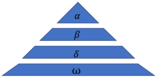
Figure 1.
Hierarchy of wolves.
2.2. Encircling the Prey
Gray wolves encircle prey during the hunt; in order to mathematically model encircling behavior, the following equations are used:
where indicates the position vector of the gray wolf, indicates the position vectors of prey, indicates the current iteration, and are coefficient vectors, and are random vectors in [0, 1] ^n, is distance control parameter, and its value decreases linearly from 2 to 0 over the course of iterations, and Max_iter is the maximum iterations.
2.3. Attacking the Prey
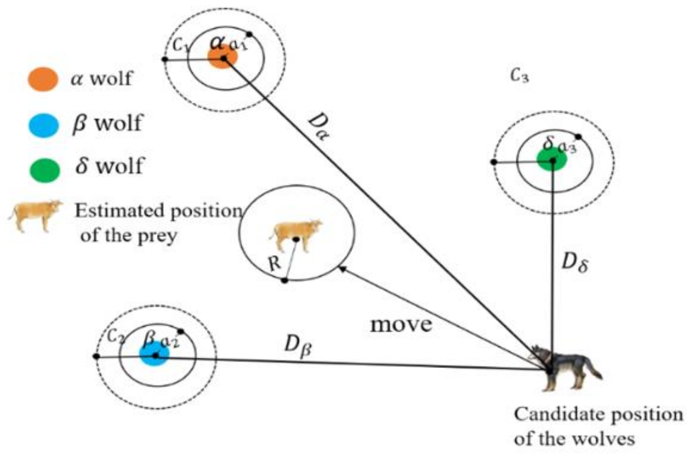
Gray wolves have the ability to recognize the location of potential prey, and the search process is mainly carried out by the guidance of , , wolves. In each iteration, the best three wolves (, ,) in the current population are retained, and then the positions of other search agents are updated according to their position information. The following formulas are proposed in this regard:
In the above equation, , and are the position vectors of α, β and δ wolves, respectively, the calculations of , and are similar to , and the calculations of , and are similar to .−, −, − represents the distance between the current candidate wolves and the best three wolves. As can be seen from Figure 2, the candidate solution finally falls within the random circle defined by and . Then, under the guidance of the current best three wolves, the other candidates randomly update their positions near the prey. They start to search the prey position information in a scattered way and then concentrate on attacking the prey.

Figure 2.
Position updating in the gray wolf optimization (GWO).
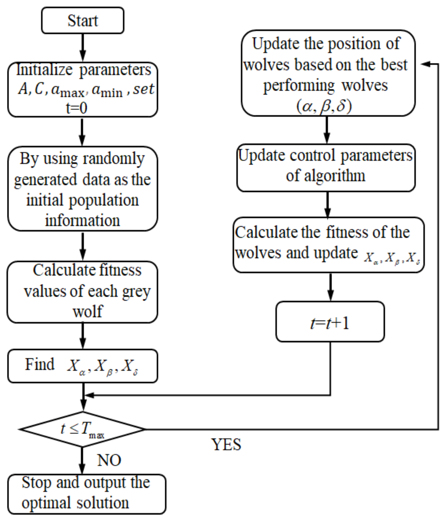
The flowchart of the GWO is given in Figure 3.

Figure 3.
GWO algorithm optimization process.
3. Improved Gray Wolf Optimization Algorithm (IGWO)
3.1. Tent Chaos Initialization
When solving practical problems, GWO usually uses the randomly generated data as the initial population information, which will make it difficult to retain the diversity of the population and lead to poor results. However, chaotic motion has the characteristics of randomness, ergodicity and regularity [27], and using these characteristics to optimize the search can maintain the diversity of the population and improve the global searchability. In general, the random motion state obtained by the deterministic equation is called chaos, and the variable representing the chaotic state is called chaotic variable. Chaos is a common phenomenon in nonlinear systems [28].
Many scholars have introduced chaotic maps and chaotic search into the GWO. The existing chaotic maps include logistic maps, tent maps, etc. However, different chaotic maps have a great impact on the chaos optimization process. At present, most of the existing chaotic maps used in the literature contain logistic maps, and the inhomogeneity of logistic traversals will affect the optimization speed, thereby reducing the efficiency of the algorithm.
Reference [29] pointed out that tent map has better ergodicity, regularity and faster speed than a logistic map. It is also proved that the tent map has a prerequisite for optimizing the chaotic sequence of algorithms by strict mathematical reasoning. Tent map is a kind of piecewise linear mapping mathematically, which is named because its function is like tent [28]. Moreover, it is a 2D chaotic map, which is widely used in chaotic encryption systems (such as image encryption), and the chaotic spread spectrum code generation, chaos encryption system construction and implementation of the chaotic optimization algorithm are also often used.
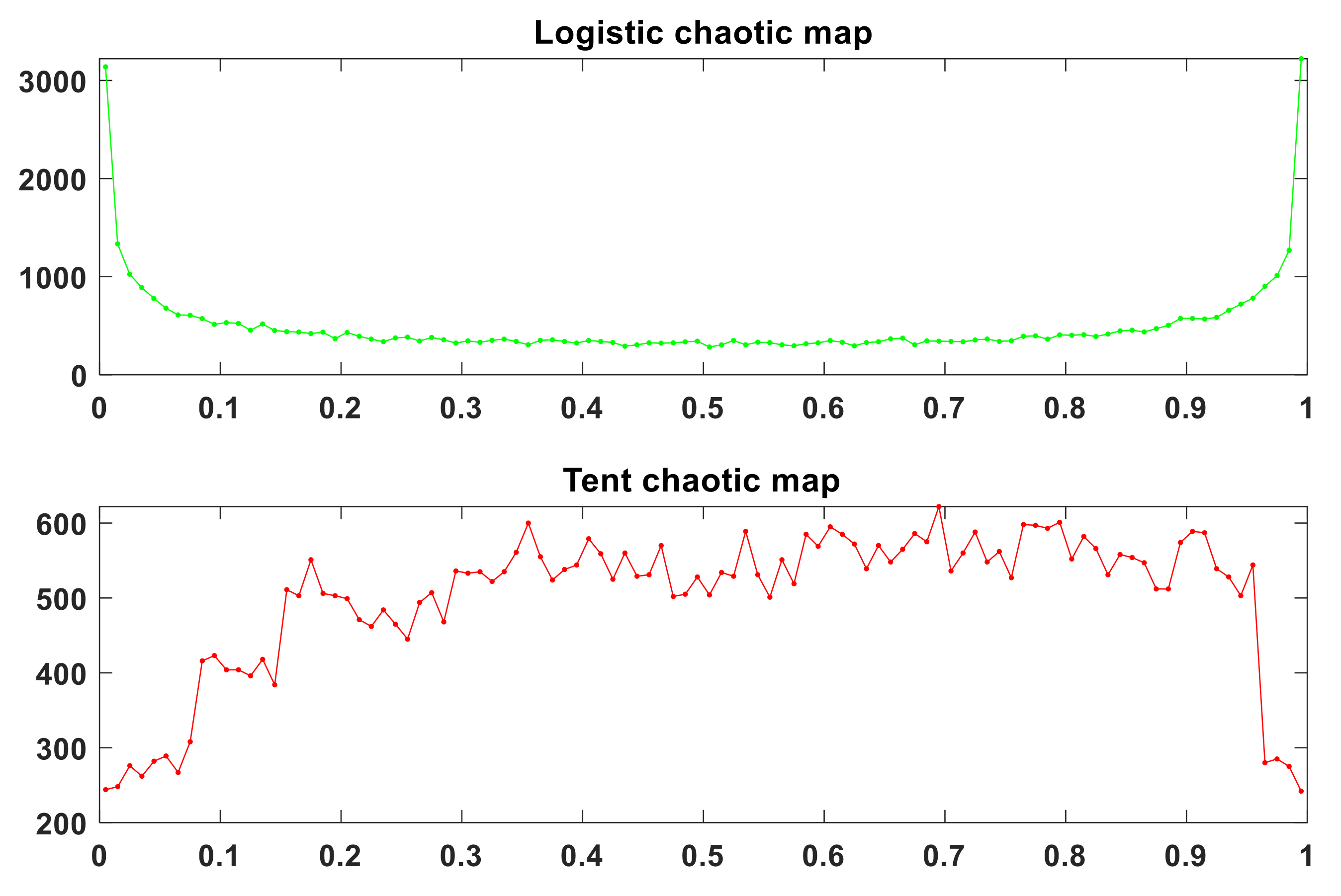
Figure 4 shows the distribution of logistic chaotic sequence and tent chaotic sequence. It can be found from Figure 4 that the probability of value in the interval of [0, 0.05] and [0.95, 1] is greater than that of other sections, and the probability of tent in each feasible region is relatively uniform. The uniformity of tent chaotic sequence generated by tent chaotic map is obviously better than that of logistic chaotic map.

Figure 4.
Chaotic sequence distribution.
In this paper, the tent chaotic map is used to optimize the search by using randomness, ergodicity and regularity, which can effectively maintain the diversity of the population, suppress the algorithm to fall into the local optima, and improve the global searchability.
In recent years, tent chaotic map has been applied to various algorithms, and good results have been achieved. Li et al. proposed a new image encryption scheme based on the tent chaotic map. They used known methods to analyze the performance and security of the proposed image encryption scheme and proved the effectiveness and security of the scheme through fault security analysis [30]. Indu et al. proposed an improved tent map particle swarm optimization algorithm (ITM-CPSO), which solved the nonlinear congestion management cost problem, realized the nonlinear congestion management cost problem of the algorithm, and further reduced the deviation of the timing pulse generator output predetermined level to reduce the overall unloading and cost [31]. Gokhale SS et al. proposed a tent chaos firefly algorithm (CFA) to optimize the time coordination of the relay, and tested it in a number of systems, obtained better results [32]. Petrovic et al. added chaotic map to the initialization of the fruit fly optimization algorithm and studied 10 different chaotic maps. The statistical results showed that FOA was improved in terms of convergence speed and overall performance [33].
The tent mapping model, which generates a chaotic sequence for population initialization, and its mathematical expression is:
Theoretical research shows that tent chaotic map is represented by Bernoulli shift transformation, as follows [29]:
where is a chaotic variable, i = 1, 2… n represents the ordinal number of chaotic variables, j = 1, 2… n represents the population size. In this paper, = 0.7.
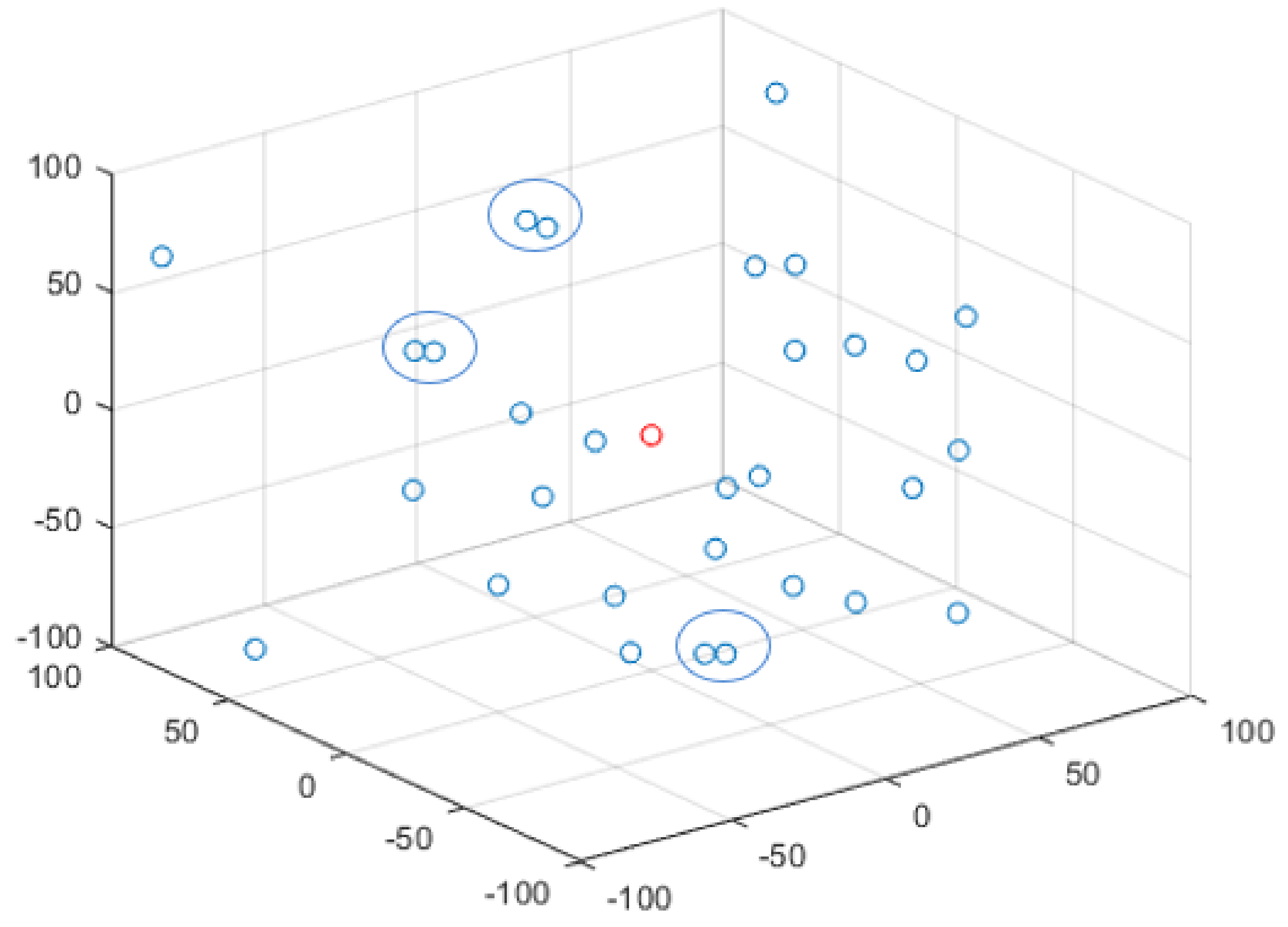
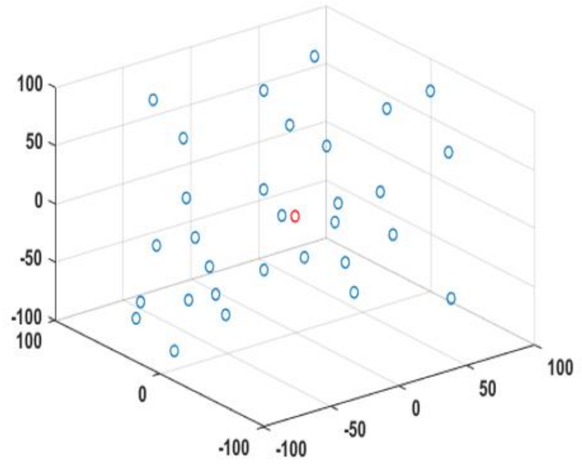
Figure 5 and Figure 6, respectively, show the initial population of the GWO and IGWO when solving the sphere function. Among them, n = 30, d = 3, and the search space range is [−100, 100]. The red circle represents the global optimal point, and the blue circle represents the gray wolf population. In the initialization phase of the algorithm, gray wolves are randomly dispersed in the search space, and the more uniform the population is, the stronger the global exploration ability will be. It can be seen from Figure 5 and Figure 6 that the tent map makes the initial population distribution more uniform, enriches the diversity of the population, reduces the probability of the algorithm falling into local optima and improves the convergence accuracy.
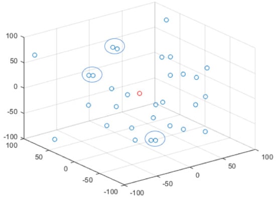
Figure 5.
Random initialization.

Figure 6.
Tent chaotic initialization.
3.2. Gaussian Perturbation
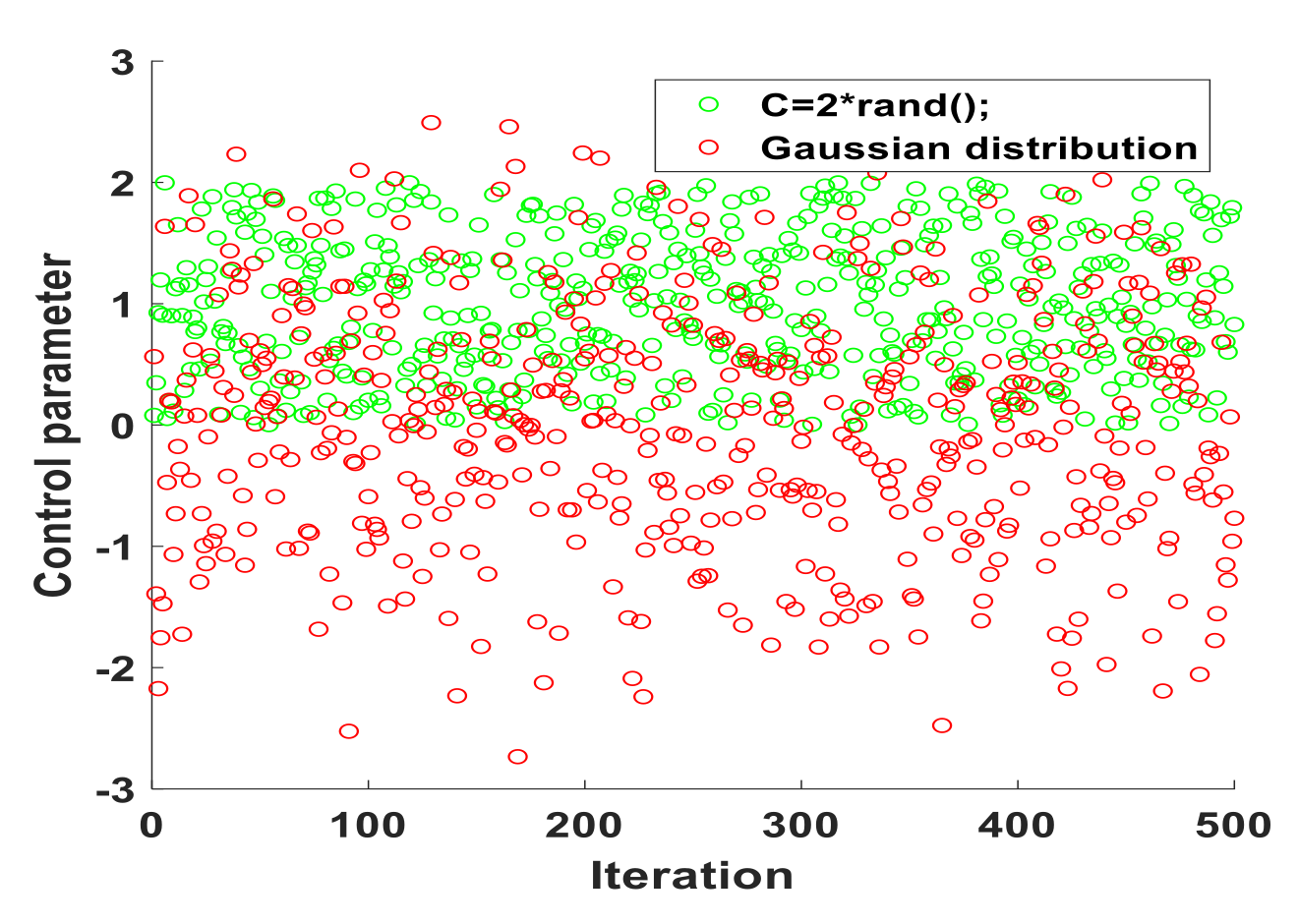
According to Equation (1), the GWO’s also plays a decisive role, Equation (3) shows that is a random vector in [0, 2], the provides random weights for prey, which can increase ( > 1) or reduce ( < 1) distance between the gray wolves and the prey. The size of helps GWO to display random search behavior during the optimization process so as to avoid the algorithm falling into local optima [16]. The leading wolf position in a population plays an important role in guiding the group to move towards the best solution. If the leading wolf’s position falls into local optima, it is easy to stop searching and lack diversity within the group. During the movement of wolves, their leading wolves were randomly generated and unpredictable. In order to avoid the premature convergence and balance the global and local exploration capabilities, the original random generation coefficient was changed to Gaussian perturbation, which will cause some perturbation to the leader and maintain the diversity of the population.
Figure 7 is the random value generated by the original and Gaussian distribution. It can be clearly seen from the figure that the random number generated by Gaussian distribution has a wider range, which can show the random walk behavior of gray wolves in the GWO algorithm more accurately.

Figure 7.
Values of Gaussian perturbations.
3.3. Cosine Control Factor
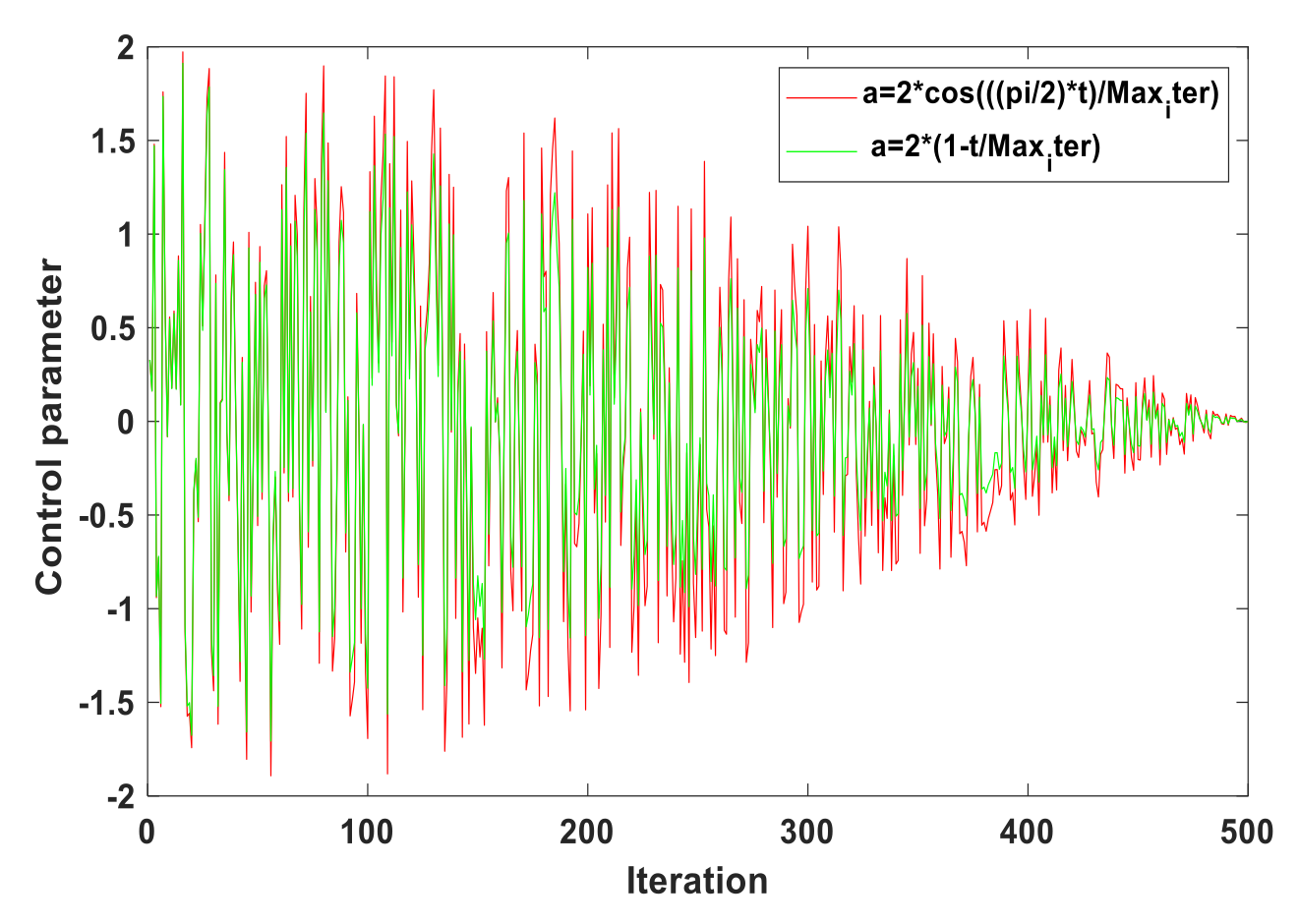
In the GWO, the coefficient vector balances the global and local search capabilities. When > 1, the gray wolves will expand the search scope, namely global searching. When < 1, the gray wolves will shrink the search scope to attack their prey, namely local search. In the early-stage of optimization, gray wolf individuals should be widely distributed in the entire search space. In the late-stage of optimization, gray wolf individuals should converge to the optimal global value by using the collected information. According to Equation (2), the attenuation factor affects the coefficient vector , which further affects the balance between GWO’s exploration and development capacity. When > 1 (the exploration stage), the gray wolves will engage in search and hunting activities, and when < 1 (the development stage), the gray wolves will only engage in hunting activities.
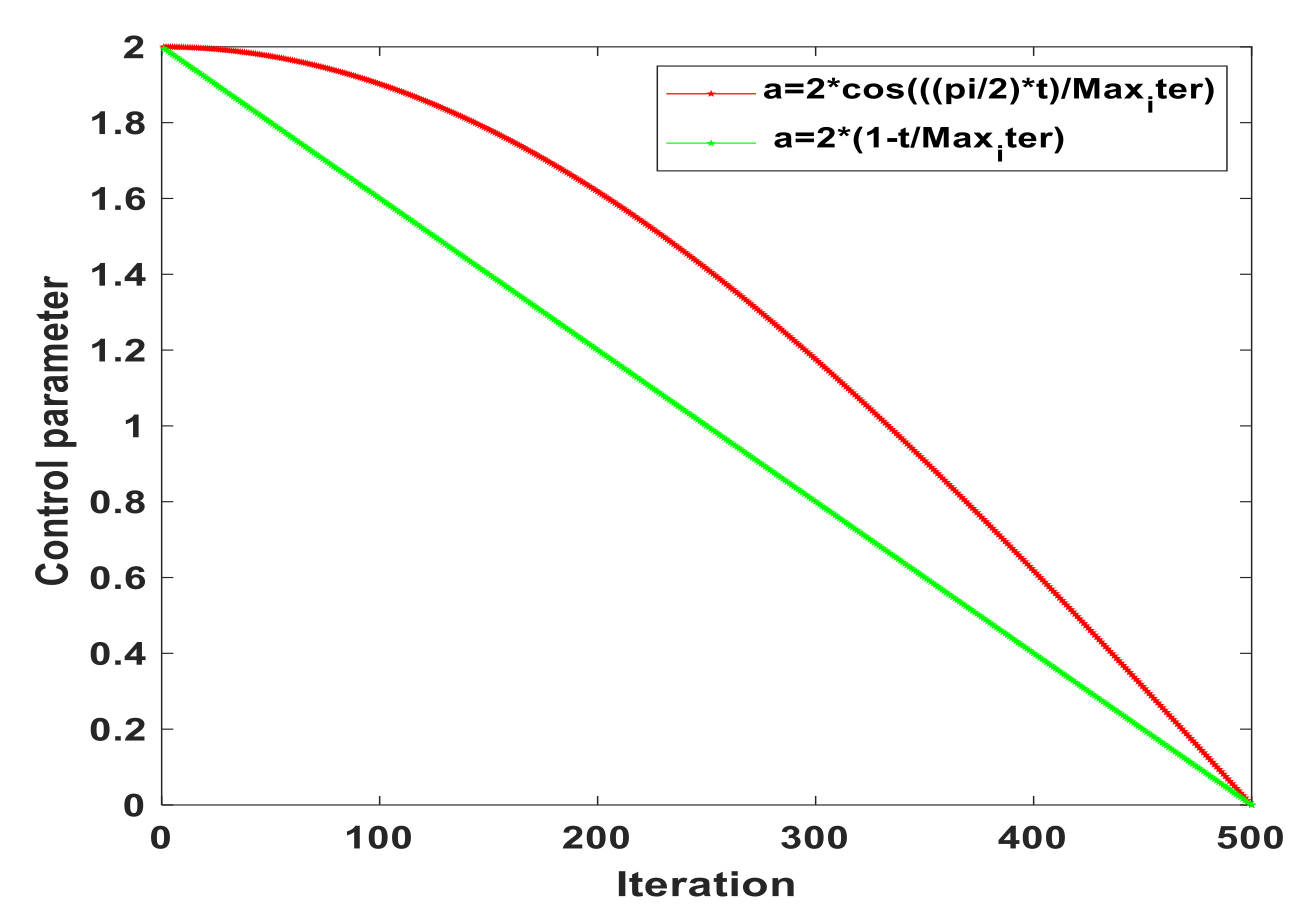
In the GWO, the convergence factor A decreases linearly with the number of iterations from 2 to 0, but the individual gray wolf does not change linearly in the process of searching prey, so the linear decline of the convergence factor A cannot fully reflect the actual optimization search process. It can be seen from Figure 8 and Figure 9, the improved and A can better reflect the actual optimization search process.

Figure 8.
Convergence curve of parameter a.

Figure 9.
Value of control parameter A.
Therefore, inspired by reference [34], the control factor of linear change is replaced by the control factor of cosine change, and its expression is as follows:
The inertia weight factor is a very important parameter [35]. When the inertia weight is large, the algorithm has a strong global searching ability, which can expand the search range. When the inertia weight is small, the local search ability of the algorithm is strong, and it can search around the optimal solution and accelerate the convergence speed.
Combined with the cosine change of the control parameter above, this paper introduces a weight cosine control factor B(t) that changes synchronously with into the position update of the GWO to further enhance the global exploration capability. With the increase of iterations, the algorithm adjustment step length becomes smaller, the global search ability gradually weakens, and the local search ability gradually strengthens. When B(t) is very small, the position of the individual population is finetuned instead of approaching the origin.
4. The Simulation Results
4.1. Optimization Function and Experimental Environment
In this section, to analyze the performance of the IGWO algorithm, 7 unimodal test functions, 6 multimodal optimization functions and 10 fixed dimensional multimodal optimization functions in reference [15] are selected. Table 1, Table 2 and Table 3 show the names, specific expressions, search space and optimal values of these functions. Among them, F1–F7 are the unimodal optimization functions, F8–F13 are the multimodal optimization functions, F14–F23 are the fixed dimensional multimodal functions. The unimodal test function is mainly used to estimate the solution accuracy and convergence speed of the IGWO, and the multimodal test function is mainly used to estimate the global surveying ability of the IGWO.

Table 1.
Unimodal optimization function.

Table 2.
Multimodal optimization function.

Table 3.
Fixed dimensional multimodal optimization function.
In order to improve the accuracy of the experiment, the 8 selected algorithms all adopt the same experimental parameters, namely, the swarm size n = 30, dimension d = 30, the maximum iterations Max_iter = 500, each algorithm is run 30 times independently and the results recorded. In, which C1 = C2 = 2, W = 0.7294 in PSO, A = 0.5, r = 0.5 in BA and P = 0.2 in FPA. In the simulation experiment, the hardware configuration of the simulation environment is Windows 10 Professional operating system; the CPU is Intel® Celeron® CPU N3060 @1.60 GHz processor, 4 GB memory, and the software configuration of the simulation environment is MATLABR2016a.
4.2. Analysis of Different Strategies
Different improvement strategies have different effects on the optimization results, and their contributions to the whole improved algorithm are also different. In order to analyze the effectiveness of the improved strategy of the IGWO algorithm, three strategies of Tent map, Gaussian distribution and cosine control factor are combined with the basic GWO, respectively, to study the influence of each strategy on the effectiveness of the algorithm. GWO1 means the combination of the GWO algorithm and tent map, GWO2 means the combination of the GWO algorithm and Gaussian distribution, and GWO3 means the combination of the GWO algorithm and cosine control factor. The test results are shown in Table 4 below.

Table 4.
Test the results of different strategies.
From Table 4, it can be seen that different strategies can improve the performance of the GWO algorithm, and GWO2 plays a greater role in improving the performance of the GWO algorithm. Overall, the combination of different strategies makes the performance of the IGWO algorithm greatly improved.
4.3. Analysis of Experimental Results
4.3.1. Compared with Other Algorithms
To further evaluate the performance of the IGWO, the IGWO algorithm was tested on 23 benchmark functions, and the results were compared with the GWO, SCA, MFO, PSO, BA, FPA and SSA 7 algorithms. The average values and standard deviation of each algorithm running 30 times are used as the evaluation criteria, and the solution with the highest accuracy is bolded in the table. The experimental test results are shown in Table 5, Table 6 and Table 7.

Table 5.
Simulation results of unimodal functions.

Table 6.
Simulation results of multimodal functions.

Table 7.
Simulation results of the fixed dimensional multimodal function.
The average values and standard deviation in Table 5, Table 6 and Table 7 can reflect the convergence accuracy and optimization capability of the IGWO. For the 7 unimodal functions, the IGWO performs better in accuracy and standard deviation when solving F1, F2, F3, F4 and F6 functions, although the optimization accuracy does not reach the theoretical optimal value of 0. For the 7 multimodal functions, the optimization accuracy reaches the theoretical optimal value 0, and the standard deviation is also 0 when solving the F9 and F11 functions, which fully demonstrates the algorithm’s solution accuracy and strong robustness. Meanwhile, compared with other optimization algorithms, the IGWO also achieves a better value when solving the F10 function. For the 10 fixed dimensional multimodal functions, F15 gets a better value than other algorithms, and the results of the remaining functions are less different from those of the contrast algorithm. It can be seen that the IGWO has advantages in solving unimodal, multimodal and fixed dimensional multimodal functions.
4.3.2. Convergence Analysis
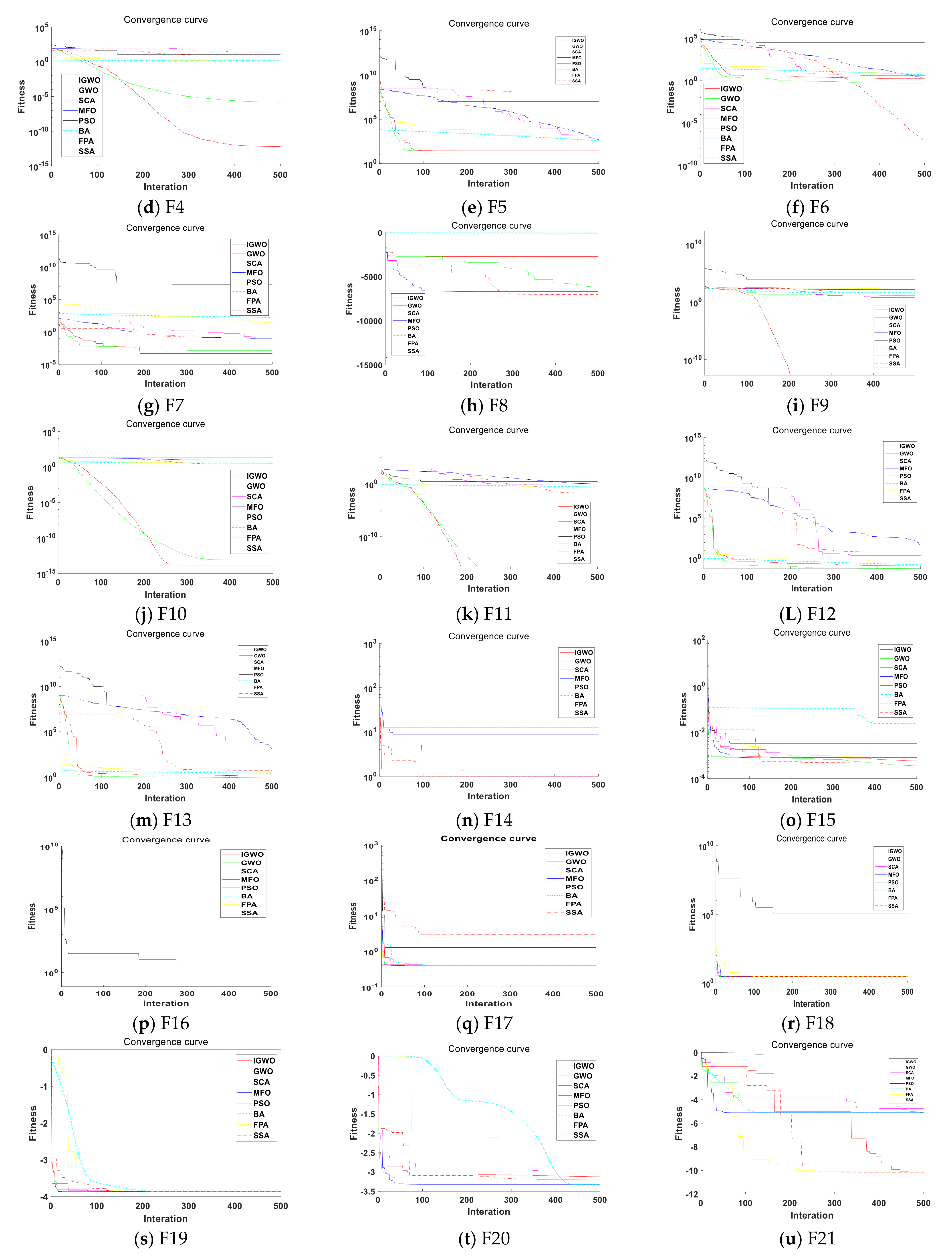
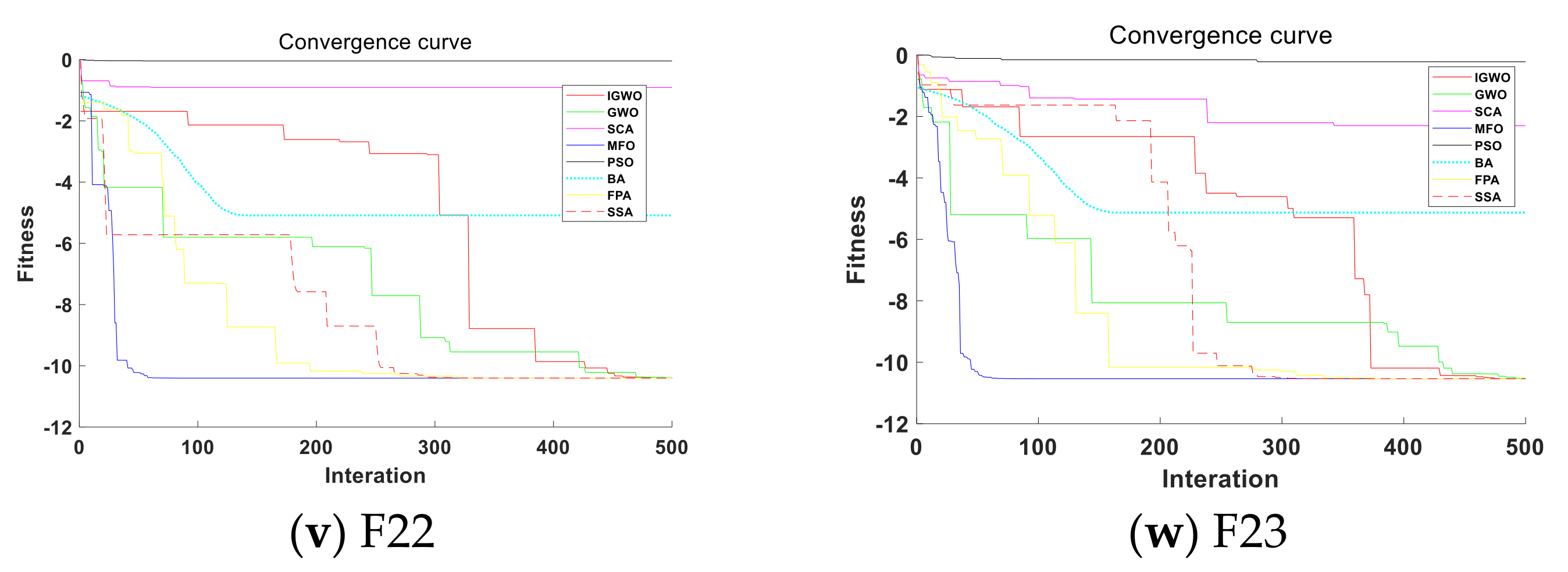
The convergence rate of the algorithm is an important index to measure the performance of the algorithm, and the algorithm convergence curve can directly compare the convergence performance of the algorithm. Figure 10a–w shows the convergence curves of fitness values of 8 algorithms, the IGWO, GWO, SCA, MFO, PSO, BA, FPA and SSA when solving 23 different types of test functions. The convergence curves are plotted by extracting the values generated by random running once when dimension d = 30.


Figure 10.
Evolution curve of the function (d = 30).
According to (a–w) in Figure 10, when solving the unimodal test function, the convergence curve of the IGWOS algorithm decreases to the lower right corner as the iterations increase, and the convergence accuracy is higher than other algorithms. Among the multimodal test functions, the IGWO tests other functions except F8 have better performance. In particular, F9 and F11 can quickly find the optimal solution with fast convergence speed and high precision. For the fixed dimensional multimodal functions, most of the function curve drops in a stepped way. This is because the algorithm keeps exploring in the iterative process, jumps out of the optimal local solution and looks for the optimal global solution, and its convergence accuracy is relatively good.
In conclusion, the IGWO algorithm combining tent maps, Gaussian distribution and control factor can fully expand the search range in the early iteration, avoid the algorithm falling into local optima, and better balance the global and local search capabilities.
4.3.3. Numerical Result Test
In this section, Wilcoxon rank-sum test [36] will be carried out on the algorithm results of 30 independent runs, and the Friedman test will be carried out on the average values in Table 5, Table 6 and Table 7. The following results were analyzed in IBM SPSS Statistics 21, and the significance level was set at 0.05. Table 8 shows the Wilcoxon rank-sum test results based on the IGWO algorithm. The bold data indicates that there is no significant difference between the comparison algorithm and the calculation results of the IGWO algorithm. Table 9 shows the rank generated by the Friedman test according to the mean values in Table 5, Table 6 and Table 7.

Table 8.
Results of the p value Wilcoxon rank-sum test on the functions.

Table 9.
The numerical results of 8 algorithms.
From Table 8, it can be concluded that the proposed IGWO significantly outperforms algorithms GWO, SCA, MFO, PSO, BA, FPA and SSA.
According to the results of Table 9, the rank means of the 8 algorithms are 2.39 (IGWO), 3.22 (GWO), 3.93 (SCA), 5.70 (MFO), 4.96(PSO), 5.73 (BA), 5.61 (FPA), and 4.37 (SSA). The priority order is IGWO > GWO > SCA > SSA > PSO > FPA > MFO > BA. IGWO compared with SCA p = 0.011 < 0.05 indicates that there is a statistically significant difference between IGWO and SCA. IGWO compared with MFO p = 0.001 < 0.05 indicates that there is a statistically significant difference between IGWO and MFO. IGWO compared with PSO p = 0.002 < 0.05 indicated that there was a statistically significant difference between IGWO and PSO. IGWO compared with BA p = 0 < 0.05 indicates that there is a statistically significant difference between IGWO and BA. IGWO compared with FPA was p = 0.01 < 0.05 indicated that there was a statistically significant difference between IGWO and FPA. IGWO compared with SSA p = 0.005 < 0.05 indicates that there is a statistically significant difference between IGWO and SSA.
5. Application to Solve Engineering Optimization Problem
In this section, four structural design problems with constraints in mechanical engineering are optimized to reduce the cost of engineering design and save resources. For these constraints, the penalty function method is used to construct the fitness function. For the objective problem , the constraint , is treated, as shown in Equation (17), is a newly constructed objective function. Both and represent a positive integer large enough (such as 10 × 1012). and are the numbers of inequality constraints and equality constraints. Parameters and take 2 and 1, respectively. When dealing with the objective problem, this method excludes all the solutions that do not meet the constraints from the candidate solutions. If the search solution satisfies the constraints, then the objective function is . When solving these engineering optimization problems, the population size n = 30, the maximum iteration number Max_iter = 500, and the results in the table are the best values obtained by running 30 times independently. The bold values indicate the best one among all methods.
5.1. Pressure Vessel Design Problem
Figure 11 shows that the objective of the pressure vessel design optimization problem is to minimize the sum of material cost, synthesis cost and welding cost while satisfying the decision variables of pressure tube thickness Ts, head cover thickness Th, inner radius R and cylindrical length. Equation (18) gives its mathematical model.
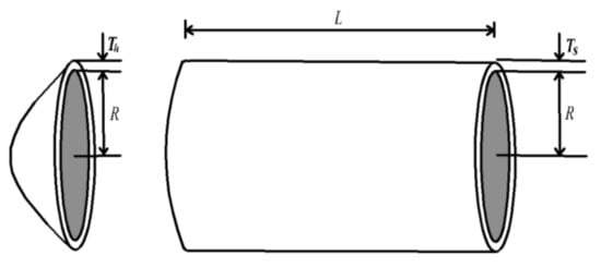
Figure 11.
Pressure vessel design problem.
Subjected to:
In order to objectively demonstrate the performance of the IGWO, the MVO in [37], GSA algorithm in [38], PSO algorithm in [39], MSCA algorithm in [40], GA (Coello) algorithm in [41], GA (Coello and Montes) algorithm in [42], GA (Deb et al.) algorithm in [43], ES algorithm in [44], DE (Huang et al.) algorithm in [45], ACO (Kaveh et al.) algorithm in [46], IHS algorithm in [47] and WOA algorithm in [48] are selected. Table 10 suggests that the IGWO finds a design with the minimum cost for this problem.

Table 10.
Comparison results of pressure vessel design problem.
According to the results of Table 10, the IGWO, obtaining the optimum cost of 5888.6000, found the best feasible optimal design among all these algorithms. Therefore, it can be concluded that the IGWO is excellent in solving the pressure vessel design problem.
5.2. Spring Design Problem
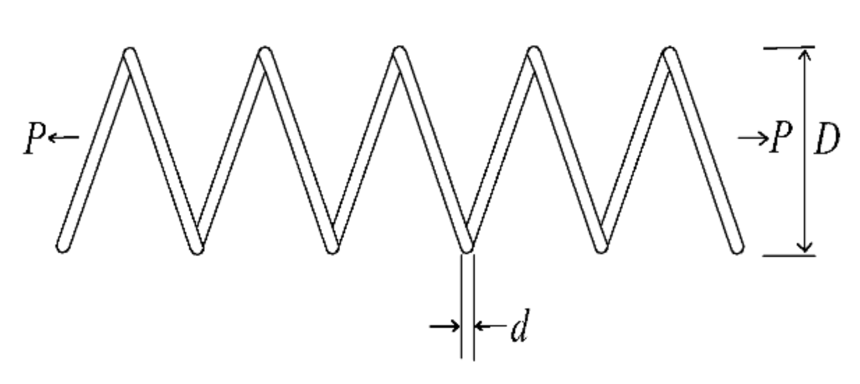
This subsection is an optimized test of the spring design problem. When the spring is applied in engineering, it is necessary to minimize the gravity of the spring and reduce the waste of materials under the setting conditions of factors, such as tortuosity, shear pressure, impact frequency and outer diameter. A schematic diagram of the spring design structure is shown in Figure 12; the effect variable is the diameter of the coil d (x1), the wire diameter D(x2), the number of effective windings P(x3). For this problem, the mathematical model of the objective function and constraint function is shown in Equation (19).
subjected to:

Figure 12.
Spring design problem.
In order to objectively demonstrate the performance of the IGWO, the mathematical optimization method (Belegundu) algorithm in [49], GSA algorithm in [38], GSA algorithm in [46], SCA algorithm in [6], and MVO algorithm in [37] are selected. The comparison results are shown in Table 11.

Table 11.
Comparison results of results for the spring design problem.
As can be seen from Table 11, the IGWO outperforms other comparison algorithms except for the GWO. However, the difference between IGWO and GWO is small.
5.3. Welded Beam Design Problem
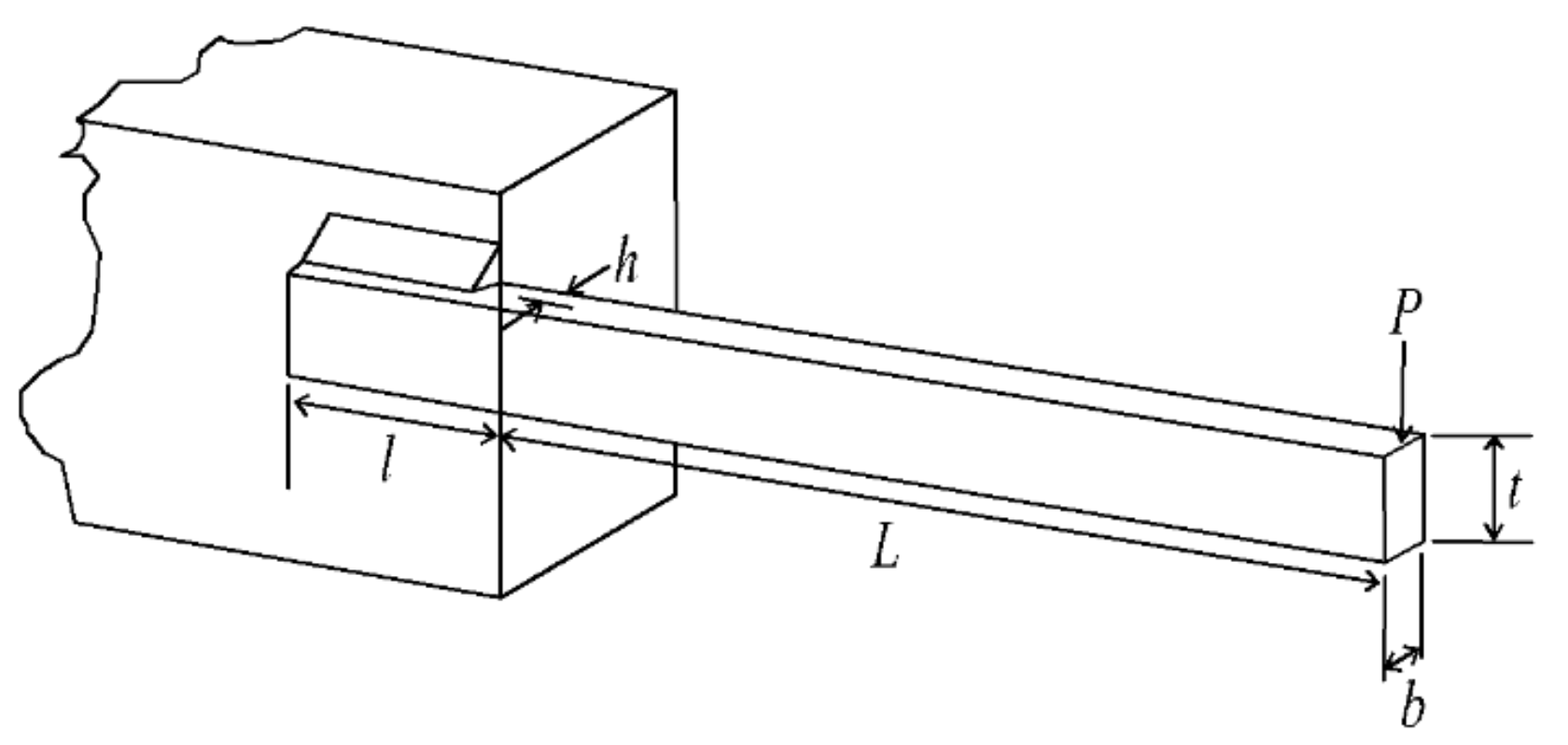
In practical engineering application, the stressed part of the engineering can be described as a welded beam design problem. That is, one end of the beam wall does not produce axial direction, does not rotate and has no vertical displacement, and the other end is a free end. As shown in Figure 13, this problem is very widespread in engineering design. The mathematical model is shown in Equation (20), where the function represents the shear stress of the joint, the bending stress of the member, the buckling stress of the member and the deflection function of the end of the member. The optimization goal of the welded beam design problem is to minimize the total manufacturing cost when the constraints are met, that is, to reduce the waste of resources.

Figure 13.
Welding beam problem.
Subjected to:
IGWO was used to solve the welding beam problem. The comparison algorithm includes NGS-WOA [50], WOA algorithm [48], RO algorithm [51], MVO algorithm [37], CPSO algorithm [52], CPSO algorithm [53], HS algorithm [54], GSA algorithm [38], GA algorithm [55], GA algorithm [56], Coello algorithm [40], and Coello and Monters algorithm [41]. The comparison results are shown in Table 12.

Table 12.
Comparison results of results for welding beam problem.
According to Table 12 statistics, the data results of each algorithm in solving the welding beam design problem; compared with the basic GWO algorithm, the solution result of the IGWO algorithm is better than that of the GWO algorithm. Judging from the results of other algorithms, the IGWO algorithm is superior to other algorithms except for MVO.
5.4. Three Truss Design Problem
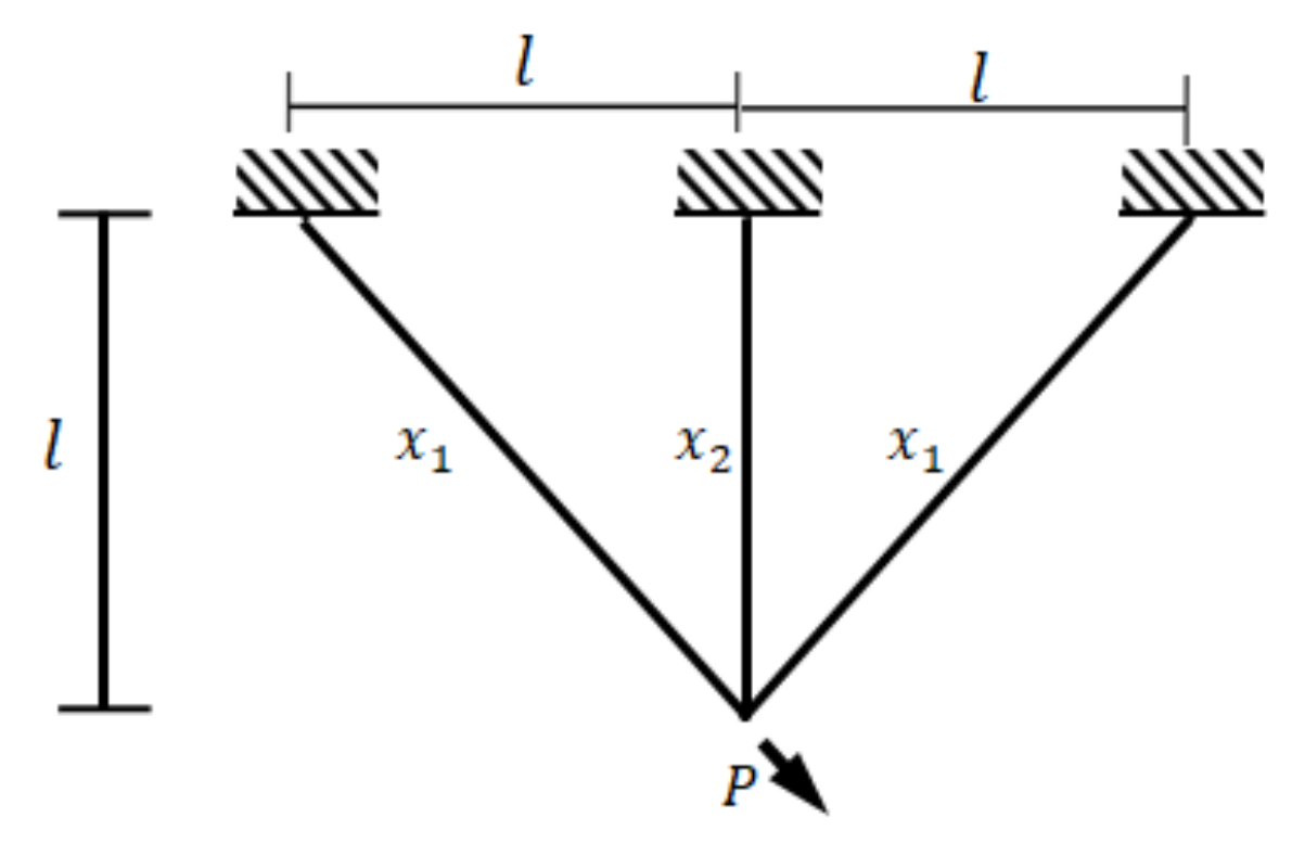
The three-truss design problem is a nonlinear optimization problem with three nonlinear inequality constraints and two continuous decision variables to minimize the cost. The goal is to optimize the cross-sectional areas of rod 1 and 3, x1, and the cross-sectional areas of rod 2, x2. The mathematical model is shown in Equation (21). The schematic diagram is shown in Figure 14.

Figure 14.
The three truss design problem.
Subjected to:
In order to objectively demonstrate the performance of the IGWO, the PSO-DE in [39], MBA algorithm in [57], DEDS algorithm in [58] CS algorithm in [59], Ray and Sain algorithm in [60], and Tsa algorithm in [61] are selected. Table 13 shows the comparison of solution results between the IGWO algorithm and other algorithms.

Table 13.
Comparison results of results for the three truss design problem.
It can be seen from Table 13 that the solution result of the IGWO algorithm is slightly inferior to the Tsa algorithm. However, compared with other algorithms, the IGWO algorithm still has some advantages. Therefore, the IGWO algorithm has certain practicability in the engineering design of three truss structures.
6. Conclusions and Future Work
To save materials and cost in the process of engineering construction, an improved gray wolf optimization algorithm termed IGWO is proposed. It combines tent chaos, Gaussian perturbation and cosine control factor to achieve a better promote the conservation and rational use of resources, alleviate the contradiction between resource supply and socioeconomic development. Twenty-three functions with different characteristics of unimodal, multimodal and fixed dimensional multimodal with different characteristics are tested, and the results are compared with seven algorithms. The experimental results show that the IGWO optimization performance and stability of the algorithm are superior to the other seven different types of comparable algorithms. Then four challenging engineering constraint optimization problems with different objective functions, constraint conditions and properties, including pressure vessel design, spring design, welded beam design and truss design, are solved. Meanwhile, the Wilcoxon rank-sum test and Friedman were used to evaluate the results of the IGWO algorithm. The experimental results show that the IGWO is more competitive than other comparison algorithms and can be an effective tool to solve engineering design problems and save resources.
For the study of this paper, the results show that the IGWO was successfully implemented to solve the practical constraints of engineering design problems. Additionally, the IGWO is able to provide very competitive results in terms of minimizing total cost. It was observed that the IGWO has the ability to converge to a better quality near-optimal solution and possesses better convergence characteristics than other prevailing techniques reported in the literature. It is also clear from the results obtained by different functions that the IGWO shows a good balance between exploration and exploitation that results in high local optima avoidance. It can be concluded that the IGWO is an effective and efficient algorithm.
However, the IGWO algorithm still has some shortcomings in some aspects, for example, it cannot be effectively applied to all problems, and the convergence accuracy can be further improved. Therefore, research on the IGWO still has much room for improvement. Our future work is divided into two parts: (1) to apply the proposed method to more practical cases to exert its full effective merits, especially in the areas of engineering optimization control; and (2) to reconstruct the proposed method as a fusion procedure with other metaheuristics to further investigate its performance thoroughly.
Author Contributions
J.L.: methodology. X.L.: resources, writing—original draft. Y.L.: writing—review and editing. All authors have read and agreed to the published version of the manuscript.
Funding
This study is supported by the National Natural Science Foundation of China (No. 71601071), the Science & Technology Program of Henan Province, China (No. 182102310886 and 162102110109), and an MOE Youth Foundation Project of Hu-manities and Social Sciences (No. 15YJC630079).
Institutional Review Board Statement
Not applicable.
Informed Consent Statement
Not applicable.
Data Availability Statement
The study did not report any data.
Acknowledgments
This study is supported by the National Natural Science Foundation of China (No. 71601071), the Science and Technology Program of Henan Province, China (No. 182102310886 and 162102110109), and a MOE Youth Foundation Project of Humanities and Social Sciences (No. 15YJC630079).
Conflicts of Interest
There are no conflicts to declare.
References
- Begum, R.A.; Siwar, C.; Pereira, J.J.; Jaafar, A.H. A benefit–cost analysis on the economic feasibility of construction waste minimisation: The case of Malaysia. Resour. Conserv. Recycl. 2006, 48, 86–98. [Google Scholar] [CrossRef]
- Huang, J.; Zhu, Y.; Kelly, J.T.; Jang, C.; Wang, S.; Xing, J.; Yu, L. Large-scale optimization of multi-pollutant control strategies in the Pearl River Delta region of China using a genetic algorithm in machine learning. Sci. Total Environ. 2020, 722, 137701. [Google Scholar] [CrossRef] [PubMed]
- Guo-Chu, C.; Jin-Shou, Y.U. Particle swarm optimization algorithm. Inf. Control 2005, 186, 454–458. [Google Scholar]
- Mirjalili, S. Moth-flame optimization algorithm: A novel nature-inspired heuristic paradigm. Knowl. Based Syst. 2015, 89, 228–249. [Google Scholar] [CrossRef]
- Mirjalili, S. The Ant Lion Optimizer. Adv. Eng. Softw. 2015, 83, 80–98. [Google Scholar] [CrossRef]
- Mirjalili, S. SCA: A Sine Cosine Algorithm for solving optimization problems. Knowl. Based Syst. 2016, 96, 120–133. [Google Scholar] [CrossRef]
- Gandomi, A.H.; Yang, X.-S. Chaotic bat algorithm. J. Comput. Sci. 2014, 5, 224–232. [Google Scholar] [CrossRef]
- Yang, X.-S. Flower Pollination Algorithm for Global Optimization. In International Conference on Unconventional Computing and Natural Computation; Springer: Berlin, Heidelberg, 2012; Volume 7445, pp. 240–249. [Google Scholar]
- Mirjalili, S.; Gandomi, A.H.; Mirjalili, S.Z.; Saremi, S.; Faris, H.; Mirjalili, S.M. Salp Swarm Algorithm: A bio-inspired optimizer for engineering design problems. Adv. Eng. Softw. 2017, 114, 163–191. [Google Scholar] [CrossRef]
- Afshar, M.H. Extension of the constrained particle swarm optimization algorithm to optimal operation of mul-ti-reservoirs system. Int. J. Electr. Power Energy Syst. 2013, 51, 71–81. [Google Scholar] [CrossRef]
- Kim, N.S.; Janic, M.; Van Wee, B. Trade-off between carbon dioxide emissions and logistics costs based on multi-objective optimization. Transp. Res. Rec. 2009, 2139, 107–116. [Google Scholar] [CrossRef]
- Lin, W.; Yu, D.Y.; Zhang, C.; Liu, X.; Zhang, S.; Tian, Y.; Xie, Z. A multi-objective teaching−learning-based opti-mization algorithm to scheduling in turning processes for minimizing makespan and carbon footprint. J. Clean. Prod. 2015, 101, 337–347. [Google Scholar] [CrossRef]
- He, Y.; Li, Y.; Wu, T.; Sutherland, J.W. An energy-responsive optimization method for machine tool selection and operation sequence in flexible machining job shops. J. Clean. Prod. 2015, 87, 245–254. [Google Scholar] [CrossRef]
- Du, B.; Zhang, J.F.; Gao, Z.H.; Li, T.; Huang, Z.Q.; Zhang, N. Based on simulated annealing particle swarm algorithm of optimal allocation of water resources research. J. Drain. Irrig. Mach. Eng. 2020, 1–10. Available online: http://kns.cnki.net/kcms/detail/32.1814.th.20200927.0952.002.html (accessed on 1 February 2021).
- Mirjalili, S.; Mirjalili, S.M.; Lewis, A. Grey wolf optimizer. Adv. Eng. Softw. 2014, 69, 46–61. [Google Scholar] [CrossRef]
- Maharana, D.; Kotecha, P. Optimization of Job Shop Scheduling Problem with Grey Wolf Optimizer and JAYA Al-gorithm. In Smart Innovations in Communication and Computational Sciences; Springer: Singapore, Singapore, 2019; Volume 669, pp. 47–58. [Google Scholar]
- Precup, R.-E.; David, R.-C.; Petriu, E.M. Grey Wolf Optimizer Algorithm-Based Tuning of Fuzzy Control Systems With Reduced Parametric Sensitivity. IEEE Trans. Ind. Electron. 2016, 64, 527–534. [Google Scholar] [CrossRef]
- Sharma, Y.; Saikia, L.C. Automatic generation control of a multi-area ST—Thermal power system using Grey Wolf Optimizer algorithm based classical controllers. Int. J. Electr. Power Energy Syst. 2015, 73, 853–862. [Google Scholar] [CrossRef]
- Shakarami, M.; Davoudkhani, I.F. Wide-area power system stabilizer design based on Grey Wolf Optimization algorithm considering the time delay. Electr. Power Syst. Res. 2016, 133, 149–159. [Google Scholar] [CrossRef]
- Yao, X.; Li, Z.; Liu, L.; Cheng, X. Multi-Threshold Image Segmentation Based on Improved Grey Wolf Optimization Algorithm. IOP Conf. Series: Earth Environ. Sci. 2019, 252, 042105. [Google Scholar] [CrossRef]
- Yang, J.C.; Long, W. Improved Grey Wolf Optimization Algorithm for Constrained Mechanical Design Problems. Appl. Mech. Mater. 2016, 851, 553–558. [Google Scholar] [CrossRef]
- Chandar, S.K. Grey Wolf optimization-Elman neural network model for stock price prediction. Soft Comput. 2021, 25, 649–658. [Google Scholar] [CrossRef]
- Bansal, J.C.; Singh, S. A better exploration strategy in Grey Wolf Optimizer. J. Ambient. Intell. Humaniz. Comput. 2021, 12, 1099–1118. [Google Scholar] [CrossRef]
- Wang, J.-S.; Li, S.-X. An Improved Grey Wolf Optimizer Based on Differential Evolution and Elimination Mechanism. Sci. Rep. 2019, 9, 1–21. [Google Scholar] [CrossRef] [PubMed]
- Teng, Z.-J.; Lv, J.-L.; Guo, L.-W. An improved hybrid grey wolf optimization algorithm. Soft Comput. 2019, 23, 6617–6631. [Google Scholar] [CrossRef]
- Zhang, S.; Luo, Q.; Zhou, Y. Hybrid Grey Wolf Optimizer Using Elite Opposition-Based Learning Strategy and Simplex Method. Int. J. Comput. Intell. Appl. 2017, 16, 1750012. [Google Scholar] [CrossRef]
- Tian, D.P. Particle Swarm Optimization Based on Tent Chaotic Sequences. Comput. Eng. 2010, 4, 180–182. [Google Scholar]
- Shan, L.; Qiang, H.; Li, J.; Wang, Z. Chaos optimization algorithm based on Tent mapping. Control Decis. 2005, 2, 179–182. [Google Scholar]
- Kennedy, J.; Eberhart, R. Particle swarm optimization. In Proceedings of the IEEE International Conference on Neural Networks, Perth, WA, Australia, 27 November–1 December 1995. [Google Scholar]
- Li, C.; Luo, G.; Qin, K.; Li, C. An image encryption scheme based on chaotic tent map. Nonlinear Dyn. 2017, 87, 127–133. [Google Scholar] [CrossRef]
- Batra, I.; Ghosh, S. An Improved Tent Map-Adaptive Chaotic Particle Swarm Optimization (ITM-CPSO)-Based Novel Approach Toward Security Constraint Optimal Congestion Management. Iran. J. Sci. Technol. Trans. Electr. Eng. 2018, 42, 261–289. [Google Scholar] [CrossRef]
- Gokhale, S.; Kale, V. An application of a tent map initiated Chaotic Firefly algorithm for optimal overcurrent relay coordination. Int. J. Electr. Power Energy Syst. 2016, 78, 336–342. [Google Scholar] [CrossRef]
- Mitić, M.; Vuković, N.; Petrović, M.; Miljković, Z. Chaotic fruit fly optimization algorithm. Knowl. Based Syst. 2015, 89, 446–458. [Google Scholar] [CrossRef]
- Huang, Q.; Li, J.; Song, C.; Xu, C.; Lin, X. A whale optimization algorithm based on cosine control factor and polynomial variation. Control Decis. 2020, 35, 50–59. [Google Scholar]
- Chatterjee, A.; Siarry, P. Nonlinear inertia weight variation for dynamic adaptation in particle swarm optimization. Comput. Oper. Res. 2006, 33, 859–871. [Google Scholar] [CrossRef]
- Derrac, J.; García, S.; Molina, D.; Herrera, F. A practical tutorial on the use of nonparametric statistical tests as a methodology for comparing evolutionary and swarm intelligence algorithms. Swarm Evol. Comput. 2011, 1, 3–18. [Google Scholar] [CrossRef]
- Mirjalili, S.; Mirjalili, S.M.; Hatamlou, A. Multi-verse optimizer: A nature-inspired algorithm for global optimization. Neural Comput. Appl. 2016, 27, 495–513. [Google Scholar] [CrossRef]
- Rashedi, E.; Nezamabadi-Pour, H.; Saryazdi, S. GSA: A Gravitational Search Algorithm. Inf. Sci. 2009, 179, 2232–2248. [Google Scholar] [CrossRef]
- Chen, H.; Wang, M.; Zhao, X. A multi-strategy enhanced sine cosine algorithm for global optimization and con-strained practical engineering problems. Appl. Math. Comput. 2020, 369, 124872. [Google Scholar]
- Coello, C.A.C.; Montes, E.M. Constraint-handling in genetic algorithms through the use of dominance-based tournament selection. Adv. Eng. Inform. 2002, 16, 193–203. [Google Scholar] [CrossRef]
- Coello, C.A.C. Use of a self-adaptive penalty approach for engineering optimization problems. Comput. Ind. 2000, 41, 113–127. [Google Scholar] [CrossRef]
- Deb, K. GeneAS: A Robust Optimal Design Technique for Mechanical Component Design. In Evolutionary Algorithms in Engineering Applications; Springer: Berlin, Heidelberg, 1997; pp. 497–514. [Google Scholar]
- Mezura-Montes, E.; Coello, C.A.C. An empirical study about the usefulness of evolution strategies to solve con-strained optimization problems. Int. J. Gen. Syst. 2008, 37, 443–473. [Google Scholar] [CrossRef]
- Huang, F.-Z.; Wang, L.; He, Q. An effective co-evolutionary differential evolution for constrained optimization. Appl. Math. Comput. 2007, 186, 340–356. [Google Scholar] [CrossRef]
- Kaveh, A.; Talatahari, S. An improved ant colony optimization for constrained engineering design problems. Eng. Comput. 2010, 27, 155–182. [Google Scholar] [CrossRef]
- Mahdavi, M.; Fesanghary, M.; Damangir, E. An improved harmony search algorithm for solving optimization problems. Appl. Math. Comput. 2007, 188, 1567–1579. [Google Scholar] [CrossRef]
- Mirjalili, S.; Lewis, A. The Whale Optimization Algorithm. Adv. Eng. Softw. 2016, 95, 51–67. [Google Scholar] [CrossRef]
- Belegundu, A.D.; Arora, J.S. A study of mathematical programming methods for structural optimization. Part I: Theory. Int. J. Numer. Methods Eng. 1985, 21, 1583–1599. [Google Scholar] [CrossRef]
- Zhang, J.; Wang, J.S. Improved Whale Optimization Algorithm Based on Nonlinear Adaptive Weight and Golden Sine Operator. IEEE Access 2020, 8, 77013–77048. [Google Scholar] [CrossRef]
- Kaveh, A.; Khayatazad, M. A new meta-heuristic method: Ray Optimization. Comput. Struct. 2012, 112–113, 283–294. [Google Scholar] [CrossRef]
- Krohling, R.A.; Coelho, L.D.S. Coevolutionary Particle Swarm Optimization Using Gaussian Distribution for Solving Constrained Optimization Problems. IEEE Trans. Syst. Man, Cybern. Part B 2006, 36, 1407–1416. [Google Scholar] [CrossRef]
- He, Q.; Wang, L. An effective co-evolutionary particle swarm optimization for constrained engineering design problems. Eng. Appl. Artif. Intell. 2007, 20, 89–99. [Google Scholar] [CrossRef]
- Sun, W.-Z.; Wang, J.-S.; Wei, X. An Improved Whale Optimization Algorithm Based on Different Searching Paths and Perceptual Disturbance. Symmetry 2018, 10, 210. [Google Scholar] [CrossRef]
- Coello, C.A.C. Constraint-handling using an evolutionary multiobjective optimization technique. Civ. Eng. Environ. Syst. 2000, 17, 319–346. [Google Scholar] [CrossRef]
- Deb, K. An efficient constraint handling method for genetic algorithms. Comput. Methods Appl. Mech. Eng. 2000, 186, 311–338. [Google Scholar] [CrossRef]
- Coello, C.A.C. Theoretical and numerical constraint-handling techniques used with evolutionary algorithms: A survey of the state of the art. Comput. Methods Appl. Mech. Eng. 2002, 191, 1245–1287. [Google Scholar] [CrossRef]
- Sadollah, A.; Bahreininejad, A.; Eskandar, H.; Hamdi, M. Mine blast algorithm: A new population based algorithm for solving constrained engineering optimization problems. Appl. Soft Comput. 2013, 13, 2592–2612. [Google Scholar] [CrossRef]
- Zhang, M.; Luo, W.; Wang, X. Differential evolution with dynamic stochastic selection for constrained optimization. Inf. Sci. 2008, 178, 3043–3074. [Google Scholar] [CrossRef]
- Gandomi, A.H.; Yang, X.-S.; Alavi, A.H. Cuckoo search algorithm: A metaheuristic approach to solve structural optimization problems. Eng. Comput. 2013, 29, 17–35. [Google Scholar] [CrossRef]
- Ray, T.; Saini, P. Engineering design optimization using a swarm with an intelligent information sharing among individuals. Eng. Optim. 2001, 33, 735–748. [Google Scholar] [CrossRef]
- Tsai, J.-F. Global optimization of nonlinear fractional programming problems in engineering design. Eng. Optim. 2005, 37, 399–409. [Google Scholar] [CrossRef]
Publisher’s Note: MDPI stays neutral with regard to jurisdictional claims in published maps and institutional affiliations. |
© 2021 by the authors. Licensee MDPI, Basel, Switzerland. This article is an open access article distributed under the terms and conditions of the Creative Commons Attribution (CC BY) license (http://creativecommons.org/licenses/by/4.0/).


