An Effective Hybrid Approach for Forecasting Currency Exchange Rates

Abstract

Accurately forecasting the movement of exchange rates is of interest in a variety of fields, such as international business, financial management, and monetary policy, though this is not an easy task due to dramatic fluctuations caused by political and economic events. In this study, we develop a new forecasting approach referred to as FSPSOSVR, which is able to accurately predict exchange rates by combining particle swarm optimization (PSO), random forest feature selection, and support vector regression (SVR). PSO is used to obtain the optimal SVR parameters for predicting exchange rates. Our analysis involves the monthly exchange rates from January 1971 to December 2017 of seven countries including Australia, Canada, China, the European Union, Japan, Taiwan, and the United Kingdom. The out-of-sample forecast performance of the FSPSOSVR algorithm is compared with six competing forecasting models using the mean absolute percentage error (MAPE) and root mean square error (RMSE), including random walk, exponential smoothing, autoregressive integrated moving average (ARIMA), seasonal ARIMA, SVR, and PSOSVR. Our empirical results show that the FSPSOSVR algorithm consistently yields excellent predictive accuracy, which compares favorably with competing models for all currencies. These findings suggest that the proposed algorithm is a promising method for the empirical forecasting of exchange rates. Finally, we show the empirical relevance of exchange rate forecasts arising from FSPSOSVR by use of foreign exchange carry trades and find that the proposed trading strategies can deliver positive excess returns of more than 3% per annum for most currencies, except for AUD and NTD.

1. Introduction

Forecasting the movement of exchange rates has long been a hot topic in various application fields, attracting the interest of academics, financial traders, and monetary authorities alike. For foreign exchange traders and stock market investors, the ability to accurately forecast exchange rates is helpful in reducing risk and maximizing returns from transactions [1,2]. From the point of view of monetary authorities, reliable exchange rate forecasting also contributes to the management of exchange rates and conduction of monetary policies. Under a managed exchange rate regime, exchange rates are allowed to fluctuate within an undisclosed band, and the authorities may intervene in this regime depending on their future expectations of the exchange rates [3]. Moreover, when a government uses monetary policies such as cutting interest rates to stimulate the economy, this will increase the income and demand for the imported goods of a country, appreciating the currency, which will ultimately negatively affect the competitiveness of exported goods. Hence, an accurate forecast of exchange rates can help a government to determine the sufficient level of interest rate cuts, which is related to evaluating the performance of monetary policies [4,5]. To accurately forecast exchange rates, academic researchers begin to study the behavior of exchange rates from a theoretical point of view. Many studies have been devoted to developing a variety of exchange rate determination models that link exchange rate levels to macro-economic variables [6,7]. The international debt theory, purchasing power parity, interest rate parity, and the asset market theory are well-known approaches that provide theoretical explanations for the relationship between exchange rates and economic fundamentals, such as a country’s balance of payments, price levels, real income levels, money supply, and interest rates, and other economic factors [8,9].

To understand whether these theories can provide a good approximation to the behavior of exchange rates, Meese and Rogoff investigated these and found that many economic forecasting models perform worse in terms of the out-of-sample forecasting of exchange rates than a simple driftless random walk (RW) model that only presumes that exchange rate forecasts are at the same level as the previous level of exchange rates [10]. The subsequent literature further indicated that during the floating exchange rate period, the relationship between the nominal exchange rate and fundamentals such as money supplies, outputs, and interest rates is clearly weak; this is referred to as the “exchange rate disconnect puzzle” [11]. Forecasting exchange rates, therefore, seems to be a difficult task.

Recent years have seen major progress in the development of sophisticated exchange rate forecasts. Ince, for example, used a specially constructed quarterly real-time dataset to evaluate the out-of-sample forecasting performance of linear models using purchasing power parity and Taylor rule fundamentals, with the former to work better at the 16-quarter and the latter at the one-quarter horizon [12]. Cavusoglu and Neveu examined the role of consensus forecast dispersion in forecasting exchange rates; they found that consensus forecasts largely appear to be unbiased predictors of exchange rates in the long run, but most do not hold in the short run [13]. Pierdzioch and Rülke examined whether the exchange rate forecasts made by experts reliably predict the future behavior of exchange rates in emerging markets; however, they obtained different results for different currencies. Their overall conclusion was that forecasts are often informative with respect to directional changes of exchange rates [14]. Dick et al. used survey data concerning forecasts collected by individual professionals and showed that good performance in forecasting short-term exchange rates is correlated with good performance in forecasting fundamentals, especially interest rates [15]. Ahmed et al. applied linear factor models that utilize the unconditional and conditional expectations of three currency-based risk factors to examining the predictability of exchange rates. They found that all the models had worse performance than a random walk with drift in out-of-sample forecasting of monthly exchange rate returns, and that the information embedded in currency-based risk factors does not produce systematic economic value for investors [16].

Recent studies suggested that the relationship between exchange rates and fundamentals may be difficult to detect using the Meese and Rogoff approach. Amat et al. discarded conventional rolling or recursive regressions to obtain exchange rate forecasts and adopted a no-estimation approach from machine leaning to show that fundamentals can provide useful information to improve forecasts at a 1-month horizon, providing an improvement in the RW model [17]. Cheung et al. comprehensively examined exchange rate forecasts from a large set of models and made a comparison of forecast performance against the RW model at various horizons by using different metrics and found that model/specification/currency combinations that could perform well in one period and one performance metric do not necessarily perform well in another period and/or performance metric [18].

Given the shortcomings of the above models, this paper adopts another approach by using machine learning (ML) to forecast changes in exchange rates. ML has received attention from academia and industry. In particular, artificial neural networks (ANNs) and statistical learning methods frequently appear in the recent exchange rate prediction literature. Several complex artificial intelligence (AI) techniques are capable of handling nonlinear and nonstationary data across various areas. Specifically, they can be used in the management of medical insurance costs [19], the refinement of multivariate regression methods [20], the management of missing IoT data [21], and the analysis of data on cancer mortality and survival [22,23].

Nosratabadi et al. conducted a comprehensive review of state-of-the-art ML and advanced deep learning (DL) methods in emerging economic and financial applications [24]. Recent novel ML methods include the following: Lin et al. exerted feature selection and ensemble learning to improve the accuracy for bankruptcy prediction. Chen et al. proposed a bagged-pSVM and boosted-pSVM for bankruptcy prediction [25]. Lee et al. used a support vector regression for the safety monitoring of commercial aircraft [26]. Husejinovic applied naïve Bayesian and c4.5 decision tree classifiers to investigate credit card fraud detection [27]. Benlahbib and Nfaoui proposed a hybrid approach based on opinion fusion and sentiment analysis to investigate reputation generation mechanisms [28]. Zhang proposed an improved backpropagation neural network to analyze and forecast the aquatic product export [29]. Sundar and Satyanarayana performed stock price prediction using multi-layer feed-forward neural networks [30]. Hew et al. applied an artificial neural network (ANN) to investigate the resistances driving mobile social commerce. Lahmiri et al. utilized ensemble learning in financial data classification [31]. Sermpinis et al. introduced a hybrid neural network structure based on particle swarm optimization and adaptive radial basis functions (ARBF-PSO), and a neural network fitness function for financial forecasting. This was achieved by benchmarking the ARBF-PSO results with those of three different neural network architectures (nearest neighbor algorithm (k-NN), autoregressive moving average model (ARMA), moving average convergence/divergence model (MACD), and naïve strategy) [32].

Recent notable hybrid DL methods include the following: Lei et al. presented a time-driven feature-aware joint deep reinforcement learning (DRL) for financial signal representation and algorithmic trading [33]. Vo et al. applied a long short-term memory (LSM) recurrent neural network to optimize socially responsible investment and portfolio decision making [34]. Moews et al. proposed a DL method based on lagged correlation to forecast the directional trend changes in financial time series [35]. Fang et al. provided a hybrid method that combined LSTM and support vector regression (SVR) on quantitative investment strategies [36]. Long et al. presented a hybrid DL scheme based on a convolutional neural network (CNN) and recurrent neural network (RNN) for stock price movement prediction [37]. Shamshoddin et al. suggested a DL-based collaborative filtering technique to predict consumer preferences in the electronic market [38]. Altan et al. promoted a DL method based on LSTM and wavelet transform (EWT) for digital currency forecasting [39]. Wang et al. proposed a hybrid method consisting of a long short-term memory network and a mean-variance model to optimize the formation of investment portfolios combined with asset pre-selection, thereby capturing the long-term dependence of financial time series data. The experiment used a lot of sample data from the British Stock Exchange 100 Index between March 1994 and March 2019. The study found that long short-term memory networks are suitable for financial time series forecasting, defeating other benchmark models by a clear advantage [40].

Recent notable ML methods in exchange rate forecasting include the following: Amat exploited ML on the fundamentals of simple exchange rate models (purchasing power parity or uncovered interest parity) or Taylor’s rule-based models to improve exchange rate forecasts. The study concluded that fundamentals contain useful information and that exchange rates are predictable even at shorter horizons [17]. Yaohao and Albuquerque’s work is based on a basic model consisting of 13 explanatory variables and analyzes spot exchange rate forecasts for ten currency pairs using support vector regression (SVR). Different nonlinear dependence structures introduced by the other nine kernel functions were tested, and the estimates were compared with a random walk benchmark. They tested the SVR model’s explanatory power gain over random walk by applying White’s Reality Check Test. Their results show that most SVR models achieve better out-of-sample performance than random walk, but they fail to achieve a statistically significant predictive advantage [41]. Zhang and Hamoir adopted random forest, support vector machine, and neural network models in four fundamental models (uncovered interest rate parity, purchasing power parity, monetary model, and Taylor’s rule model). They used six different maturities of government bonds and four price indices to perform an integrated robustness test. Their findings show that the basic model incorporating modern ML has superior performance in predicting future exchange rates compared to the effects of random walks [42]. Galeshchuk’s work discovered artificial neural networks’ economic purpose via describing and empirically testing foreign exchange market data. Panel data on exchange rates (USD/EUR, JPY/USD, USD/GBP) were examined and optimized for time series forecasting with neural networks. The best neural network with the best predictive power was found based on specific performance metrics [43]. For DL methods, the deep belief network (DBN) model based on DL is a new forecasting method of exchange rate data. Its structure design and parameter learning rules are essential parts of the DBN model. Shen proposed an improved DBN for exchange rate forecasting. The DBN was constructed using a continuous restricted Boltzmann machine (CRBM), and the conjugate gradient method was used to accelerate learning. Weekly GBP/USD, BRL/USD exchange rates, and INR/USD exchange rate return values were predicted by the improved DBN [44]. Zheng et al. conducted research, analyzed the results of training analysis, set up the nodes, adjusted the number of hidden nodes, input nodes, and hidden layers, and used multivariate analysis of variance to determine the sensitive range of the nodes. Finally, experiments on Indian Rupee/US dollar and RMB/US dollar exchange rates show that the improved DBN model can better predict the exchange rate than the feed-forward neural network model [45]. Go and Hong employed DL to forecast stock value streams while analyzing patterns in stock prices. In the study, a deep neural network DL algorithm was designed to find patterns using time series techniques, which achieved high accuracy. The results were assessed by the percentage of the test set of 20 firms. An accuracy value of 86% was obtained for the DNN [46].

Deep reinforcement learning (DRL) features scalability and has the potential to be applied to high-dimensional problems by combining noisy and nonlinear patterns of economic data. According to Mosavi et al.’s comprehensive review paper, the use of deep reinforcement learning in economics is proliferating [47]. DRL opens vast opportunities for addressing complex dynamic economic systems through a wide range of capabilities from reinforcement learning (RL) to DL. A comprehensive survey revealed that DRL could offer better performance and higher efficiency than conventional algorithms while facing real economic problems in the face of increasing risk parameters and uncertainty [47]. Recently emerging studies related to the use of DRL in economics include the following works. Zhang et al. used a DRL algorithm to design a trading strategy for continuous futures contracts. They compared their algorithm with a classical time series momentum strategy and showed that the study’s approach outperforms the baseline model and can lead to positive profits, but with the limitation of high transaction costs [48]. The applications of deep deterministic policy gradient (DDPG) and deep Q-network (DQN) have received much attention in recent years. Xiong et al. introduced a DDPG-based DRL approach for stock trading [49]. Li et al. proposed an adaptive DRL method based on DDPG for stock portfolio allocation [50]. Liang used DDPG-based DRL in portfolio management [51]. Li et al. presented a DQN-based DRL method to conduct an empirical study on efficient market strategy [52]. Azhikodan introduced a stock trading bot based on a recurrent convolutional neural network (RCNN) and DRL [53]. The applications of DRL in portfolio management also include advanced strategy in portfolio trading [54] and dynamic portfolio optimization [55]. Furthermore, online services’ application involves recommendation architecture [56] and pricing algorithms for the online market [57].

The literature review indicates that ML and DL have been widely used in economics research in stock markets, cryptocurrencies, marketing, corporate insolvency, and e-commerce. It reflects that ML and DL methods have received attention from economics in recent years, and the trends reveal that hybrid models outperform other single learning algorithms. A future trend will be the development of complex hybrid DL models [24].

Although the predictive performance of these nonlinear AI methods is reported to surpass that of econometric models, issues such as hyperparameter optimization and overfitting may pose difficulties [58]. For statistical learning methods, Vapnik developed a support vector machine (SVM) and successfully applied this to classification and regression problems in a variety of research fields such as tourism management, marketing, and bioinformatics [59,60,61,62,63]. SVM is one of the most established methods in statistical learning. In particular, SVM based on the radial basis function (RBF) kernel has been widely utilized to deal with nonlinear problems. Support vector regression (SVR) is a closely related statistical learning approach and can be considered the application of SVM to regression. It is based on the theory of structural risk minimization (SRM) and minimizes errors on the basis of generalized errors. Therefore, SVR can theoretically guarantee that the optima it finds are global ones; neural network models, by contrast, easily fall into local optima. However, SVR needs appropriate model parameters to work effectively [64,65].

Recently, hybrid SVR models using evolutionary algorithms have also attracted much attention because of their promising predictive performance [64,66,67]. Nevertheless, a hybrid SVR with hyperparameter optimization may not be able to meet robustness criteria. Moreover, several studies have shown that ML methods such as SVR and ANN are less accurate than conventional time series models for the problem of univariate time series with one-step prediction [68,69]. Clearly, there is still room for improvement in the accuracy of exchange rate forecasting. Feature selection is also a topic currently of great interest in machine learning. The feature selection method based on ensemble learning has received particular attention. This method, in which many different classifiers are generated as feature selectors and total results are then aggregated, is superior to the conventional single-feature selection method in several respects, most outstandingly in its ability to deal with robustness issues that often thwart existing single-feature selection methods [70]. Hence, this study develops a new SVR-based forecasting approach named FSPSOSVR, in order to accurately predict exchange rates. It is known that the benefits of artificial intelligence approaches depend on the use of appropriate parameter settings. Although different methods have been proposed to determine a suitable set of parameter values, there is still a lack of comprehensive guidelines for empirical researchers wishing to obtain robust results [71]. To alleviate the negative effect of parameter settings on our empirical results, we combine particle swarm optimization (PSO), ensemble feature selection, and SVR to forecast the exchange rates. FSPSOSVR uses an ensemble feature selection mechanism. Compared to conventional single-feature selection techniques, ensemble feature selection has the advantage of robustness and shows great promise for use with high-dimensional samples of small size [72]. More specifically, we used the random forest method, an ensemble approach based on a bagged strategy that samples a subset from the entire dataset to train the classifier. Several studies have shown that the random forest algorithm is robust to noise data [73,74]. As the monthly exchange rate is a dataset with a high dimension and small sample size, we expect FSPSOSVR to excel in robustness and predictive power.

Our analysis was conducted using the monthly data of exchange rates from January 1971 to December 2017 for seven countries. The out-of-sample forecast performance of the FSPSOSVR is compared with six competing forecasting models through the use of mean absolute percentage error (MAPE) and root mean square error (RMSE), including RW, exponential smoothing (ETS) [75], autoregressive integrated moving average (ARIMA) [76], seasonal ARIMA (SARIMA), SVR [77], and PSOSVR. The contribution of this paper is in synthesizing the SVR model with an evolutionary mechanism, the PSO algorithm, which adjusts the SVR hyperparameters, and also in integrating it with a feature selection mechanism based on ensemble learning. Our algorithm was able to discover the exchange rates and achieve accurate and stable performance despite the nonlinearity of the problem. The robustness of the proposed algorithm was demonstrated by comparison with empirical results. To conclude, this approach incorporates foreign exchange carry trades to demonstrate the empirical relevance of exchange rate forecasts and specifically demonstrates the practicality of this approach for exchange carry trades. This work’s findings can contribute to the sustainability of business operations and the effective implementation of the central bank’s monetary policy to maintain a sustainable economic performance. For business sustainability, the findings can be applied to exchange rate risk management, enhancing foreign exchange risk visibility to reduce operational risk. The accurate currency forecasts can improve the profitability of carrying trade and achieve sustainable return performance. In terms of the sustainability of economies, the findings can design monetary policies to curb inflation, stabilize the consumer price index (CPI), achieve full employment and gross domestic product (GDP) growth, stabilize national economies, and promote stable economic growth.

2. Materials and Methods

2.1. Overview of Techniques

In order to accurately predict the exchange rate, a hybrid model named FSPSOSVR is proposed, which consists of random forest (RF), PSO, and SVR. In the FSPSOSVR model, the reliable lag variable is identified using RF, the approximate optimal coefficient of SVR is obtained by PSO, and SVR is used as the prediction model. The above techniques are introduced as follows.

2.1.1. Support Vector Regression

Vapnik et al. introduced support vector machines (SVMs) to solve classification problems [78]. Support vector regression (SVR) is an SVM-based algorithm proposed by Drucker for regression applications [77]. The basic function of SVR is to find a nonlinear function that maps training data to a high-dimensional feature space.

Given a training dataset {(x_i, y_i); i = 1, 2, …, N}, where each x_i ∈ X ∈ Rⁿ, x_i is the ith input, X represents the input sample space, the match true output is y_i ∈ Rⁿ, and N is the size of the dataset. The estimation function is defined as

$$y=f(x_i)=w^T\phi (x_i)+b,$$

(1)

where w ∈ R^m and b ∈ Rⁿ are adjustable coefficients, and φ(x) represents a nonlinear function from Rⁿ to the high-dimensional space R^m(m > n). The penalty function R(C) is defined by using the penalty function to estimate the values of the coefficients w and b as

$$R(C)=\frac{1}{2}{\Vert w\Vert }^2+C\cdot \frac{1}{n}{\displaystyle \sum _{i=1}^n{\left|y_i-f(x)\right|}_{\epsilon }},$$

(2)

$${\left|y-f(x)\right|}_{\epsilon }=\{\begin{array}{c}0,\hfill \\ \left|y-f(x)\right|-\epsilon ,\end{array}\begin{array}{l}\left|y-f(x)\right|\le \epsilon ,\\ \mathrm{otherwise} \end{array},$$

(3)

where C is the penalty factor and ε is the maximum value of tolerance [79]. By introducing two relaxation variables ${\xi }_i$ and ${\xi }_i^{*}$, (2) can be rewritten as

$$\begin{array}{l}\underset{w,b,{\xi }_i^{(*)}}{\min }\frac{1}{2}{\Vert w\Vert }^2+C{\displaystyle \sum _{i=1}^n\left({\xi }_i+{\xi }_i^{*}\right)}\\ \mathrm{subject}\mathrm{to}\{\begin{array}{l}-y_i+w^T\varphi (x_i)+b\le \epsilon +{\xi }_i,\\ y_i-w^T\varphi (x_i)-b\le \epsilon +{\xi }_{{}_i}^{*},\\ {\xi }_i^{(*)}\ge 0,\end{array}\begin{array}{c}(i=1,\dots ,m)\\ (i=1,\dots ,m)\\ (i=1,\dots ,m)\end{array}\end{array}$$

(4)

where the value for ξ_i⁽*⁾ ensures that the constraint listed in the second expression is met, C controls the balance between the model complexity and training error rate, and ε is the constant that controls the tube size, which is traded off against the model complexity and slack variables. If ε is too small, overfitting may occur, while the opposite case may result in underfitting. Finally, by introducing the Lagrange multiplier and using the optimality constraint, the decision function shown in (5) is obtained.

$$\begin{array}{l}\underset{{\alpha }_i,{\alpha }_i^{*}}{\min }\frac{1}{2}{\displaystyle \sum _{i,j=1}^n{y}_i\left({\alpha }_i-{\alpha }_i^{*}\right)\left({\alpha }_j-{\alpha }_j^{*}\right)k\left(x_i,x_j\right)}+{\displaystyle \sum _{i=1}^n\left(\left(\epsilon -y_i\right){\alpha }_i+\left(\epsilon +y_i\right){\alpha }_i^{*}\right)}\\ \mathrm{subject} \mathrm{to} \{\begin{array}{l}{\displaystyle \sum _{i=1}^N\left({\alpha }_i-{\alpha }_i^{*}\right)}=0,\\ 0\le {\alpha }_i^{(*)}\le C, (i=1,\hspace{0.17em}\hspace{0.17em}\dots ,m)\end{array}\end{array}$$

(5)

The SVR function can be used to solve (5) as follows:

$$f(x)={\displaystyle \sum _{i=1}^n\left({\alpha }_i-{\alpha }_i^{*}\right)}k\left(x_i,x\right)+b,$$

(6)

where ${\alpha }_i$ and ${\alpha }_i^{*}$ are the Lagrange multipliers, and k(x_i, x_j) is a kernel function. In the SVR input space, the kernel function establishes a nonlinear decision hypersurface. The Gaussian radial basis function (RBF) kernel is the most widely used kernel. This not only performs nonlinear mapping between the input space and high-dimensional space, but is also easy to implement in the solution of nonlinear problems. The Gaussian RBF kernel can be formulated as

$$k\left(x_i,x\right)=\exp \left(-\sigma {\Vert x-x_i\Vert }^2\right),$$

(7)

where σ represents the Gaussian RBF kernel scaling factor.

2.1.2. Particle Swarm Optimization

Particle swarm optimization (PSO) is a population-based stochastic search algorithm proposed by [80] and has been successfully applied in several fields [81,82,83,84,85]. The first step in PSO is the choice of a randomly initialized solution. Each feasible solution is treated as a “particle” and represented by a point in the D-dimensional space, where D is the number of parameters to be optimized. The position and velocity of the ith particle are expressed as vectors $x_i=\left(x_i,1, \dots , x_i,D\right)$ and $v_i=\left(v_i,1, \dots , v_i,D\right)$, where $i=1, 2,\dots , n.$. Each particle is a potential solution to the problem in the D-dimensional search space. These particles share information with each other, and the search direction of each particle can be altered to adjust its search to a more promising search area. Each particle has its own best experience, defined in the feature space as the best known position of the particle i (pbest_i), and the best experience derived from the population is expressed as the best known position (gbest) in the population. In each generation, each particle is accelerated to pbest_i and gbest. The empirical value is evaluated using the fitness function f(x) according to the problem definition. In the feature space, the position and speed must be limited between a reasonable lower bound and an upper bound. The updated speed and position can be determined using the following equation:

$$v_{i,d}^{new}=w{v}_{i,d}^{old}+c_1{r}_1\left(pbes{t}_{i,d}-x_{i,d}\right)+c_2{r}_2\left(gbes{t}_d-x_{i,d}\right),$$

(8)

where w is the inertial weight, $c_1$ and $c_2$ are the acceleration constants, and $r_1$ and $r_2$ are uniform random values between 0 and 1. The inertia weight w controls the current speed,

$$x_i^{new}=x_i^{old}+v_i^{new}\hspace{0.17em},$$

(9)

where $w_{\max }$ is set to 0.9, $w_{\min }$ is set to 0.4, and max_iter and iter are the maximum and current iterations, respectively [80].

$$w=w_{\min }-\left(w_{\max }-w_{\min }\right)\times \frac{iter}{max\_iter},$$

(10)

All operations in the PSO are repeated until the termination condition is reached. The termination condition corresponds to the maximum range of the iterative operation. The PSO algorithm is described in Algorithm 1.

2.1.3. Selecting SVR Parameters Using PSO

In SVR modeling, parameter settings affect the performance of the predicted time series, as described in the above discussion of PSO. The key parameters are the regularization parameter (C), kernel function bandwidth (σ), and tube size of the ε-insensitive loss operator (ε). Incorrect selection of parameter values can result in overfitting or underfitting [86]. Therefore, once an SVR is used to forecast the time series, it is important to select optimal parameters. In this paper, the three parameters of the SVM model are approximated using PSO. The PSOSVR model program procedure is as follows:

Step 1: 

Initialization. The parameters of the particle are randomly initialized. Each particle i is expressed as x_i = {C, σ, ε}.

Step 2: 

Fitness evaluation. After the encoding process is completed, the values of parameters C, σ, and ε are inserted into the SVR model for forecasting, and k-fold cross-validation (CV) is used in the training phase to avoid overfitting and to calculate the verification error. CV is mostly used in applied machine learning to measure the performance of a machine learning model’s skill based on an unseen dataset. The PSOSVR model uses a rolling-based process to forecast data. The process is used as prediction schemes and maintains time series to avoid overfitting in the machine learning models and the time series models [87]. A fixed window is used in the process, and the value in the fixed window is updated with each newly predicted value. This process involves removing historical data and adding future data so that the fixed window always retains the same amount of time series data, and the forecast accuracy is computed by averaging over the test sets with criteria. First-in/first-out (FIFO) is an updating strategy in rolling forecasting; this type of strategy is also referred to as a continuous or recursive strategy. An example of FIFO for rolling forecasting is illustrated in Figure 1.

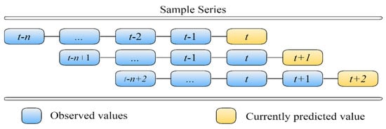Figure 1. The sequences for observed value and predicted value in rolling-based forecasting.

Algorithm 1: Particle swarm optimization algorithm.

The top twelve lagged observation data points are used as input variables, and the current data are used as the output variables. First, enter the first twelve exchange rate datasets into the model. On this basis, a predictive value of the next month is obtained. The new twelve data points are scrolled forward to include the test value of the next month and are input into the model to obtain a second predicted value. This process is repeated until all the predictions in the training set are obtained, and the verification error is then calculated. This study used the mean absolute percentage error (MAPE) as the fitness function.

Step 3: 

Update pbest. If the fitness value of particle i in the current iteration exceeds pbest_i, then pbest_i is replaced by x_i.

Step 4: 

Update gbest. If the pbest_i fitness value in the current iteration exceeds gbest, replace gbest with pbest_i.

Step 5: 

Update the velocity. The velocity of each particle is updated by (8).

Step 6: 

Update the position. The position of each particle is updated by (9).

Step 7: 

Stop criteria. These processes are repeated in the order described above until the maximum number of iterations is reached.

2.1.4. Random Forest

RF is an integrated learning method for classification and regression problems [88]. The principle of RF is to combine a set of binary decision trees. Forecasting is conducted using most of the trees (in the classification) to vote or to average their output (in the regression). In addition to classification and regression, RF provides an internal measure of variable importance by calculating importance scores. Similarly, it can be used to select key features. In the process of constructing an RF, each node of the decision tree is split into two sub-nodes, and the segmentation criterion is used to reduce the impurity of a node, which is measured by the importance of its Gini [88]. In the process of node folding, i is the impurity of the node, and the importance of the node’s Gini is defined as

$$i=1-{\displaystyle \sum _j{p}^2\left(j\right)},$$

(11)

where p(j) is the proportion of samples marked j in this node. The impurities of the node after folding are described as follows

$$\Delta i=i_{parent}-\left(p_{left}\times i_{left}+p_{right}\times i_{right}\right),$$

(12)

where p_left and p_right are the sample proportions of the left and the right child nodes, respectively, and i_parent, i_left, and i_right are the Gini importance of the parent node, left child node, and right child node, respectively. For any one feature X_i, the sum of the impurity reductions in all the decision trees is the Gini importance of X_i:

$$\alpha \Delta I={\displaystyle \sum _k\Delta i_k},$$

(13)

This equation represents the importance of each feature, with larger values indicating the more important features. Recursive feature elimination (RFE) is a recursive process based on feature sorting. According to a feature sorting criterion, the RFE starts with a complete set, then deletes the least relevant features at once, selecting the most important features. This study used a feature selection (FS) method that combines RFE and RF, called RF–RFE. This process is described in Algorithm 2.

Algorithm 2: Random forest–recursive feature elimination (RF–RFE).

2.2. The Hybrid Model: FSPSOSVR

We proposed a prediction model, FSPSOSVR, to determine the most effective feature subset and improve the prediction performance of FSPSOSVR. Figure 2 illustrates the calculation process, where the specific steps are as follows:

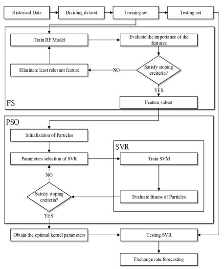
Figure 2. FSPSOSVR algorithm. The flowchart illustrates the proposed FSPSOSVR algorithm. The upper part FS expresses feature selection; the bottom part PSO represents particle swarm optimization.

Step 1: 

The dataset is divided into a training set and a test set. The training set is used as the original subset F.

Step 2: 

The subset F is used to train the RF model, and the variable importance scores of each feature in the subset are calculated.

Step 3: 

The least important feature is eliminated from F and Step 2 is repeated until the desired number of features is obtained.

Step 4: 

The PSOSVR process is initiated after allowing the new training to be integrated into the feature subset F obtained by RF–RFE.

2.3. Overview of Benchmarking Models

2.3.1. Random Walk

The random walk model is a well-known prediction method usually used as a benchmark for many various competitive models, including univariate time series, unconstrained vector autoregression, and structure models based primarily on the monetary theory of Meese and Rogoff [1]. In the random walk model, the current forecast value of exchange rates is totally based on the previous level of exchange rates as follows:

$$F_t=x_{t-1},$$

(14)

where F_t is the predicted value of the exchange rate at time t and X_t−1 is the observed value at time $t-1$.

2.3.2. Exponential Smoothing (ETS)

Exponential smoothing (ETS) is a data averaging method that considers the three factors of error, trend, and season. Maximum likelihood estimation (MLE) is used to optimize the initial values and parameters, and the optimal exponential smoothing model is selected. In addition, the weight of the ETS weighted data is exponentially decayed, the weight of the latest data is the highest, and the weight of the latter data is gradually reduced. The ETS algorithm overcomes the limitations of the previous exponential smoothing model and fails to provide a convenient way to calculate the prediction interval [89]. This paper uses the ETS algorithm proposed by [87] and implements it through the R package.

2.3.3. Autoregressive Integrated Moving Average (ARIMA)

ARIMA is a popular time series forecasting method proposed by Box and Jenkins [90], in which the exchange rate data are differenced to ensure they are stationary before estimation by an ARMA model. The ARIMA contains three parameters, p, d, q, which represent the autoregressive order, differencing, and moving average order in the model. The predicted value of exchange rates is calculated as follows:

$$F_t={\varphi }_1{X}_{t-1}+{\varphi }_2{X}_{t-2}+\cdot \cdot \cdot +{\varphi }_p{X}_{t-p}+{\epsilon }_t+{\theta }_1{\epsilon }_{t-1}+{\theta }_2{\epsilon }_{t-2}+\cdot \cdot \cdot +{\theta }_q{\epsilon }_{t-q},$$

(15)

where $F_t$ is the predicted value at the t period; ${\varphi }_i, i=1,\dots , p$ is the ith autoregression parameter; ${ϵ}_t$ is the error term at the t period; and ${\theta }_i, i=1,\dots , q$ is the ith moving average parameter. MLE is used to estimate these parameters.

2.3.4. Seasonal ARIMA (SARIMA)

When the exchange rate contains seasonality, we remove the seasonal effect from the data by taking the seasonal differencing. This leads to introducing the seasonal ARMA model, denoted by ARIMA (p, d, q)(P, D, Q)s, where p is the order of non-seasonal AR processes, q is the order of non-seasonal MA processes, d is the difference order, P is the order of seasonal AR processes, Q is the order of seasonal MA processes, and D is the seasonal difference order [76]. The general form of SARIMA is written as follows:

$${\varphi }_p(B){\Phi }_p(B^s){\nabla }^d{\nabla }_S^D{F}_t={\Theta }_Q(B^s){\theta }_q(B){\xi }_t,$$

(16)

where ${\varphi }_p\left(B\right)$ is a non-seasonal AR operator, ${\Phi }_p\left(B^s\right)$ is a seasonal AR operator, ${\Theta }_Q\left(B^s\right)$ is a seasonal MA operator, ${\theta }_q\left(B\right)$ is a non-seasonal MA operator, B is the backshift operator, ${\nabla }^d$ is the non-seasonal dth differencing, ${\nabla }_s^D$ is the seasonal dth differencing at s number of lags, $F_t$ is the forecast value for period t, and s equals 12 months in this study.

2.3.5. Backpropagation Neural Network

Backpropagation neural networks (BPNNs) are among the best-known neural networks. They have found applications in many research fields [91]. A BPNN learns a function $f(.)=R_i\to R_o$ from a dataset by a backpropagation algorithm, where i and o are the number of dimensions of the input and output feature vectors, respectively. Given input data $X=x_1,x_2,\dots , x_D$ and a target $y_i$, a BPNN can learn a nonlinear function for classification or regression. One or more hidden layers for capturing nonlinear features may be placed between the input and output layers of the BPNN. The set of neurons $\left\{x_i\right|x_1,x_2,\dots , x_i\}$ composing the input layer represents an input feature vector. Each hidden layer transforms the values passed from the previous layer using a weighted linear summation followed by applying an activation function. Finally, the output layer aggregates the results from the previous layers and transforms them into an output vector [92]. In our algorithm, only one neuron is used in the output layer; it represents the predicted value of exchange rates.

2.3.6. Forecast Performance Criteria

In order to evaluate the forecast performance of FSPSOSSVR, two common statistical measures, root mean square error (RMSE) and MAPE, are used in this study by comparing the deviation between the actual and forecast values. The metrics RMSE and MAPE are described in (17) and (18), respectively.

$$\mathrm{RMSE}=\sqrt{\frac{1}{N}{\displaystyle \sum _{i=1}^N{\left(y_i-f_i\right)}^2}},$$

(17)

$$\mathrm{MAPE}=\frac{1}{N}{\displaystyle \sum _{i=1}^N\left|\frac{y_i-f_i}{y_i}\right|}\times 100\%,$$

(18)

where y_i is the actual value, f_i is the forecast value, and N is the sample size. The lower the RMSE and MAPE values, the higher the forecast accuracy, indicating that the predicted values are reliable.

2.4. Model Specification Settings

RF, PSO, and SVR are the parameters that must be determined under the FSPSOSVR scheme. For RF, the default value provided in the scikit-learn package is used [93], the number of trees is set to 100, and the Gini function is used to measure the quality of a split. For PSO, the standard setting suggested by Bratton and Kennedy [94] is used. The size of the population is set to 50, acceleration factors $c_1$ and $c_2$ are both set to 2.0, and the maximum number of iterations (max_iter) is set to 100. For SVR, the search spaces of the SVR parameters are set to C = [2⁰, 2¹, 2³…, 2¹⁰], σ = [2⁻⁸, 2⁻⁷, 2⁻⁶…, 2⁰], and ε = [2⁻⁸, 2⁻⁷, 2⁻⁶…, 2⁰]. All main parameters in the used methods are presented in Table 1.

Table 1. Main parameters of all methods.

Methods	Main Parameters
ETS	The four main parameters for ETS, $\alpha , \beta , \gamma$, and $\varphi$, are constrained to a domain between 0 and 1. The parameters are estimated using the ets function in the forecast package in R [95].
ARIMA	The three main parameters, p, d, and q, represent the autoregressive, differential, and moving average orders, respectively.
SARIMA	The three main parameters, P, D, and Q are applied to seasonal trend modeling. P is the order of seasonal AR processes, Q is the order of seasonal MA processes, and D is the seasonal difference order. The values of the main parameters used in the ARIMA and SARIMA methods, determined by Box and Jenkins [90], are implemented via the auto. arima function in the forecast package in R [95].
ANN	The main parameters are the default parameters of the multi-layer perceptron (MLP) in the scikit-learn package [93]. The hidden layer size is set to 100; the activation function is set to use the rectified linear unit.
SVR	The radial basis kernel is used as the kernel function. The cost of a constraint violation (between 0 and 1) is determined using PSO.
PSOSVR	The size of the population is set to 50. Acceleration factors $c_1$ and $c_2$ are both set to 2.0. The parameter settings in the SVR component of PSOSVR are the same as for SVR.
FSPSOSVR	The number of trees in RF is set to 100, and the Gini function is used to measure the quality of a split. The parameter settings in the PSOSVR component of FSPSOSVR are the same as for PSOSVR.

3. Results and Discussion

3.1. Datasets and Preprocessing

This study uses monthly data for seven major exchange rates, including the Australian dollar (USD/AUD), British pound sterling (USD/GBP), Canadian dollar (CAD/USD), Chinese renminbi (RMB/USD), euro (USD/EUR), Japanese yen (JPY/USD), and new Taiwan dollar (NTD/USD). The sample periods for the exchange rates have different start dates but the same end date of 2017:M12, due to data availability. The Australian, Canadian, Japanese, and British data start from 1971:M1; the euro data start from 1999:M1. The data for China and Taiwan data start from 1981:M1 and 1984:M1, respectively. All the data were collected from the International Monetary Fund’s International Financial Statistics, detail refer to the Supplementary Materials.

We use monthly rather than quarterly or annual data in this paper because the monthly observations are evidently more frequent and therefore more numerous, and because this article concerns the medium- and long-term behavior of the exchange rate. Monthly data have been used in the literature, e.g., by Cavusoglu and Neveu [13], and by Chinn and Moore [96]. We chose five of the seven currencies studied (the Australian dollar, British pound sterling, Canadian dollar, euro, and Japanese yen) because they are the most popular currencies for trading in the foreign exchange market. We also studied the renminbi (RMB) because, with the economic development in China, it has become increasingly important in the foreign exchange market: according to Wikipedia, the RMB is a major reserve currency of the world and has become the eighth most traded currency. The NTD was included because Taiwan’s annual import and export value exceeds 60% of its GDP, and exchange rate changes affect the performance of imports and exports. Hence, the behavior of the NTD may display a different pattern than the major traded currencies.

The monthly data for the seven exchange rates are displayed in Figure 3. As shown in the figure, each currency shows different patterns of movement. For example, the Australian dollar against the US dollar began to appreciate after it reached the lowest point in 2002; the euro showed an appreciation trend before 2008, and after 2008, it showed a trend of depreciation; the yen has a clear appreciation trend after 1980, and the trend of appreciation has remained until now. Further, the financial crisis that occurred at the end of 2008 severely affected the behavior of all currencies. The implementation of fiscal and monetary policies in various countries will affect the exchange rate behavior of the countries. Overall, each series of data shows varying degrees of variations, making it difficult to predict basing on economic fundamentals. Table 2 displays the descriptive statistics of monthly currencies for the seven countries, including the minimum, maximum, mean, standard deviation, coefficient of variance (CV), and observations for each currency. In Table 2, the yen shows the highest degree of variation in terms of its CV value of approximately 45.5. The new Taiwan dollar has the lowest CV value of all the currencies, implying a lower variability in the foreign exchange market of Taiwan.

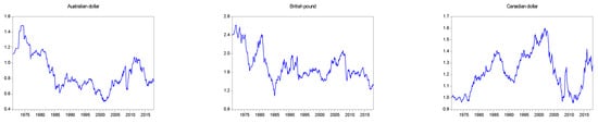
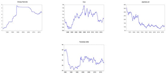
Figure 3. Time series plots of monthly nominal exchange rates.

Table 2. Descriptive statistics of monthly exchange rates.

Country	Min	Max	Mean	Med	Q1	Q3	IQR	SD	CV (%)	OBS
Australia	0.502	1.486	0.877	0.789	0.719	1.053	0.334	0.227	25.86	564
Canada	0.955	1.600	1.218	1.204	1.058	1.350	0.292	0.167	13.68	564
China	1.552	8.725	6.154	6.591	4.734	8.277	3.543	2.160	35.06	564
Euro	0.853	1.576	1.208	1.229	1.085	1.332	0.248	0.172	14.25	408
Japan	76.643	358.020	161.600	123.745	108.067	226.791	118.724	73.600	45.50	444
Taiwan	24.770	40.501	31.208	31.226	28.101	33.150	5.049	3.741	11.97	564
UK	1.093	2.618	1.742	1.642	1.536	1.881	0.345	0.314	18.02	228

Abbreviations: Min = minimum, Max = maximum, Med = median, Q1 = first quartile, Q3 = third quartile, IQR = interquartile range, SD = standard deviation, CV = coefficient of variance, OBS = observation. Note: CV (%) is defined as the ratio of the standard deviation to the mean; a larger value indicates a larger variance.

Furthermore, each dataset is divided into two subsets: the training and test sets. The training set is used for training the model, consisting of monthly data points for the whole data range between 1971 and 2017. The test set is used for testing the forecast accuracy and consists of the monthly data for 2017. Table 3 shows the results of the forecast performance evaluation that we obtained using time series models, including RW (random walk), ETS, ARIMA, and SARIMA, as well as ML methods such as SVR, PSOSVR, and FSPSOSVR. Results using the SARIMA and ETS models are obtained using the auto.arima and ets functions of the R forecast package [97]. The Python module sklearn.svm, which is an interface of the LIBSVM library [98], is used to obtain results from the SVR-based models. RMSE and MAPE are employed to compare the out-of-sample forecasting performance of the models. The smaller the value of RMSE and MAPE, the higher the prediction accuracy. For the sake of illustrating the differences between these models, we also calculate the average forecast performance of each model. Driftless RW is the benchmark model.

Table 3. Out-of-sample forecast performance evaluation for monthly data.

Country	Criteria	Random Walk	ETS	ARIMA	SARIMA	ANN	SVR	PSOSVR	FSPSOSVR
Australia	MAPE (%)	4.177	6.305	4.866	4.948	5.443	5.326	4.947	3.410 *
	RMSE	0.036	0.053	0.041	0.042	0.048	0.045	0.042	0.030 *
Canada	MAPE (%)	3.380	3.637	3.261	3.261	3.057	5.931	3.187	2.872 *
	RMSE	0.053	0.058	0.052	0.052	0.052	0.084	0.048	0.045 *
China	MAPE (%)	2.455	2.455	2.773	2.773	2.968	2.632	2.523	1.076 *
	RMSE	0.207	0.207	0.230	0.230	0.257	0.223	0.211	0.092 *
Euro	MAPE (%)	6.469	8.247	7.005	7.005	5.020	7.225	4.474	3.701 *
	RMSE	0.090	0.111	0.096	0.096	0.068	0.103	0.066	0.049 *
Japan	MAPE (%)	3.459	10.572	2.987	4.602	2.299	2.227	2.131	1.622 *
	RMSE	4.106	12.316	3.802	5.264	2.919	3.034	2.615	2.095 *
Taiwan	MAPE (%)	5.246	6.342	5.772	5.933	2.553	4.509	4.266	1.551 *
	RMSE	1.649	1.996	1.808	1.864	0.812	1.410	1.340	0.574 *
UK	MAPE (%)	3.436	4.566	3.670	4.075	3.885	4.549	2.809	1.837 *
	RMSE	0.054	0.071	0.057	0.064	0.060	0.574	0.040	0.026 *
Avg	MAPE (%)	4.089	6.018	4.333	4.657	3.603	4.628	3.477	2.296 *
	RMSE	0.885	2.116	0.869	1.087	1.144	0.782	0.623	0.416 *

* Indicates a significant statistical difference between FSPSOSVR and other models. Bold indicates the best results. Bold: the superior values.

Table 3 shows noticeable improvements in RW for all seven currencies, yielding lower RMSE and MAPE values than RW. Taking the Australian dollar as an example, the FPSOSVR’s MAPE and RMSE are 3.410 and 0.030, respectively, lower than the values of 4.177 and 0.036 that are obtained with RW, and the relative predicted performances (the ratio of MAPEs and RMSEs) are 0.816 and 0.313, respectively. Overall, the FPSOSVR’s average forecast performance compares favorably with RW, providing MAPE and RMSE values of 2.296 and 0.416, respectively, which are much lower than the values of 4.089 and 0.885 for RW. Further comparison of FSPSOSVR and SVR models (PSOSVR and SVR) reveals that the prediction accuracy of the FSPSOSVR model can consistently outperform the SVR models for all currencies. The gains in terms of the MAPE and RMSE compared to SVR models are significant. From the average forecast performance, the ratio of the MAPE (RMSE) of FSPSOSVR to PSOSVR is 0.660 (0.668) and the ratio of MAPE (RMSE) of FSPSOSVR to SVR is 0.496 (0.532), all of which are less than one. Further, as shown in Table 3, FSPSOSVR still has an excellent predictive accuracy compared to the ETS, ARIMA, and SARIMA models for all the tested currencies, consistently providing the lowest MAPE and RMSE values. In terms of the average accuracy of FSPSOSVR, the ratio of its MAPE (RMSE) to that of ETS is 0.382 (0.197); the ratio of its MAPE (RMSE) to that of ARIMA is 0.530 (0.529); the ratio of its MAPE (RMSE) to that of SARIMA is 0.493 (0.383).

Comparing the results of the RW and SVR models, it is found that the average prediction accuracy of RW (RMSE) is higher than that of the SVR model, but lower than that of the PSOSVR model. The ratios of its MAPE (RMSE) to that of the SVR and PSOSVR models are 0.884 (1.132) and 1.176 (1.421), respectively. Finally, comparing RW with the time series models, the average prediction accuracy of RW is higher than that of the three models for almost all cases, which is consistent with the literature. Compared with the three models, the relative prediction performance of the RW model is less than 1; the ratios of their MAPEs (RMSEs) are 0.679 (0.418), 0.944 (1.018), and 0.878 (0.814), respectively.

3.2. Comparison of Time Series Models and SVR-Based Models

We used the MAPE and RMSE for each method in Table 3 to demonstrate the predictive abilities of the two kinds of predictive models: time series and artificial intelligence methods. Compared with the time series models, it is not necessary for the artificial intelligence models to determine whether the data are stationary, nor do these consider whether other statistical tests should be used, instead learning from the characteristics of the training data. The three artificial intelligence methods described in this paper are superior to the time series models in the majority of cases in terms of out-of-sample predictive ability. In addition, the FSPSOSVR method outperforms the PSOSVR and SVR methods in solving prediction problems. The overall prediction accuracy of the different models is illustrated in Figure 4. The blue histograms in the figure represent the mean MAPE for each model, and the orange histograms represent the mean RMSE. The means of MAPE and RMSE for FSPSOSVR are shown to be less than those for any other model, implying that the FSPSOSVR model exhibits the best performance.

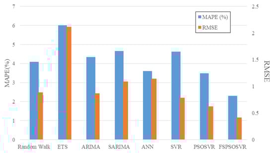
Figure 4. Overall average exchange rates forecast accuracy for the eight models.

3.3. Comparison of PSOSVR and FSPSOSVR

To increase the forecasting accuracy of our proposed algorithm, the FS method was employed. RF–RFE was used to identify the reliable lagged variables. To determine the appropriate number of features, this study tested four to eight features to determine the optimal number. The lagged variables are presented in Table 4, and y_t−i indicates the exchange rate level i months ago. As shown in Table 4, although the numbers of each country’s input variables are twelve lagged variables, only the six most relevant lagged variables are selected by the FSPSOSVR method. The selected lagged variables vary from country to country, depending on the currency characteristics. For example, FSPSVR selected the lagged variables y_t−12, y_t−10, y_t−4, y_t−3, y_t−2, and y_t−1 for Australia, while it selected y_t−8, y_t−5, y_t−4, y_t−3, y_t−2, and y_t−1 for Japan. In addition, for all currencies, the recent lagged exchange rate values (y_t−2, y_t−1) were chosen commonly, implying they are closely related to the current exchange rates at time t and hence are helpful to obtain an accurate forecast of the exchange rate. Since the method FSPSOSVR could select the most relevant input variables, it is not necessary to use all of the input variables. FSPSOSVR has a higher prediction efficiency and produces a more accurate forecast value of the exchange rates. The results indicate that after applying FS, the prediction ability was superior to that of PSOSVR (without FS). Additionally, by removing the input variable with the least influencing power, a more suitable result was obtained.

Table 4. Lagged variables of FSPSOSVR.

Country	Lagged Variables
Australia	yt−12, yt−10, yt−4, yt−3, yt−2, yt−1
Canada	yt−11, yt−7, yt−4, yt−3, yt−2, yt−1
China	yt−12, yt−11, yt−6, yt−5, yt−2, yt−1
Euro	yt−8, yt−7, yt−4, yt−3, yt−2, yt−1
Japan	yt−8, yt−5, yt−4, yt−3, yt−2, yt−1
Taiwan	yt−9, yt−7, yt−6, yt−3, yt−2, yt−1
UK	yt−12, yt−10, yt−4, yt−3, yt−2, yt−1

3.4. Forecasting Accuracy Statistics Test

As discussed by Diebold and Mariano [96] and Derrac et al. [99], the Wilcoxon signed-rank test [100] and the Friedman test [101] are reliable statistical benchmarks. They have been widely applied in studies of ML models [66,67,102]. We used both methods to compare the forecasting accuracy performance of the proposed FSPSOSVR model to the performances of the ARIMA, SARIMA, ETS, SVR, ANN, and PSOSVR models. Both statistical tests were simultaneously implemented with a significance level of $\mathsf{\alpha }=0.05$. The results in Table 3 show that the proposed FSPSOSVR model could provide a significantly better outcome in terms of forecasting performance than the other models.

Beyond evaluating the model performance on the basis of the MAPE and RMSE, a series of pairwise hypothesis tests was considered in the application of the model confidence set (MCS) framework proposed by Hansen et al. (2011) to the construction of a set of the superior model set (SMS) [103], which cannot reject the null hypotheses of the equivalent predictive power. The relative performance of the models was estimated according to the assumption of the equivalent predictive power, which tests whether the pairwise loss is different from zero averaged over time for all model combinations. In the present study, a test statistic was constructed to evaluate this assumption and implement this procedure using the MCS package in R [104]. In accordance with the default settings of the packages, α = 0.15 and 5000 bootstrap replications were performed. The set with the equivalent predictive power that we arrived at is shown in Table 5. The results indicate that it is possible to generate multiple best models for each country using the MCS. However, for all seven exchange rate datasets, FSPSOSVR was present within the SMS. This demonstrates that the FSPSOSVR scheme is robust in its forecasting ability.

Table 5. The equivalent predictive power of the model set M was equivalent (α = 0.15).

Country	Superior Model Set
Australia	Random walk, FSPSOSVR
Canada	PSOSVR, FSPSOSVR
China	Random walk, ETS, FSPSOSVR
Euro	PSOSVR, FSPSOSVR
Japan	PSOSVR, FSPSOSVR
Taiwan	ANN, FSPSOSVR
UK	PSOSVR, FSPSOSVR

Superior Model Set: In each set of models, although their forecasting performance surpassed that of all the excluded models, the null hypothesis of the equivalent predictive power cannot be rejected.

3.5. Structural Forecasting Models of Exchange Rates

3.5.1. Single Forecasting Equations

In this section, we introduce three famous structural models of exchange rates to forecast the exchange rates. These models come from the standard international economics and have been extensively examined in the literature [6,17], including the uncovered interest parity (UIRP) [105], the purchasing power parity (PPP) [106], and the simple monetary model (MM) [107,108]. The UIRP argues that the interest rate differential between home and foreign countries is equal to the changes in the exchange rate over the same time period [105]. PPP can be viewed as an international version of the law of one price, postulating that a common basket of goods and services, expressed in a common currency, costs the same between two countries [106]. Hence, if PPP holds, it will imply that there is a long-run relationship between the nominal exchange rate and the price differential between two countries. The simplest monetary model states that exchanges rates can be modeled as linear combinations of changes in money stocks and outputs between home and foreign countries [107,109]. In detail, the adopted forecasting model of the exchange rate using the fundamentals is given by

$$s_t=\alpha +\beta f_t+e_t,$$

(19)

where $s_t$ is the logarithm of the exchange rate at time t, $f_t$ is the fundamentals, and $e_t$ is the regression error. $\alpha$ and $\beta$ are parameters to be estimated. Here, the fundamentals $f_t$ are specified according to the structural models and have the form

$$\mathrm{UIRP}: f_t=i_t-i_t^{*}$$

(20)

$$\mathrm{PPP}: f_t=p_t-p_t^{*}$$

(21)

$$\mathrm{MM}: f_t=(m_t-m_t^{*})-(y_t-y_t^{*}).$$

(22)

where $i_t$, $p_t$,$m_t$, and $y_t$ denote the home country’s nominal interest rate, price level, money stock, and output in natural logarithms. Asterisks indicate foreign (i.e., US) variables. We estimate Equation (19) by the ordinary least square (OLS) method and conduct a forecast for each currency.

3.5.2. Multivariate Forecasting Equations

We continue to formulate the forecasting models by fitting the exchange rate and fundamentals with a vector autoregression (VAR) model when the two series are stationary, or a vector error correction model (VECM) when the two series are non-stationary but cointegrated. Then, forecasts are made accordingly by the estimated VAR/VECM models. The basic p-lag VAR(p) has the form

$$y_t=A_0+A_1{y}_{t-1}+A_2{y}_{t-2}+\dots +A_p{y}_{t-p}+u_t,\hspace{1em}t=1,\dots ,T.$$

(23)

where $y_t={(s_t,f_t)}^{\prime }$ denotes a $2\times 1$ vector of the exchange rate and fundamentals, respectively, and $u_t$ represents white noise processes that may be contemporaneously correlated. $A_0$ is the constant vector, and $A_i$ represents $2\times 2$ coefficient matrices. Since that each equation in Equations (5) and (23) has the same regressors, consisting of lagged values of $s_t$ and $f_t$, the VAR model can be estimated by the OLS equation.

If the exchange rate and fundamentals are non-stationary without cointegration, then a VAR model is fitted with the differences in the data. On the other hand, if the two series are non-stationary but cointegrated, we fit a vector error correction model (VECM) in which an error correction term is included in the VAR specification of differenced data and has the form

$$\Delta y_t=\alpha {\beta }^{\prime }{y}_{t-1}+{{\rm B}}_1\Delta y_{t-1}+\dots +{{\rm B}}_{p-1}\Delta y_{t-p+1}+u_t,\hspace{1em}t=1,\dots ,T.$$

(24)

where parameter $\alpha$ measures the speed of adjustment towards the long-run equilibrium; $\beta$ is the long-run coefficient matrix; ${\beta }^{\prime }{y}_{t-1}$ is the error correction term, reflecting the long-term equilibrium relationship between variables. Forecasts are generated from both estimated VAR/VECM models in a recursive manner.

3.5.3. Data Sources

The paper used monthly observations of the nominal exchange rate, money supply, industrial production index, consumer price index, and nominal interest rate for the seven countries, where the US is designated as the foreign country. Due to the limited data, the sample period for China has been changed from 1993M1 to 2018M9, and it remains unchanged for the other countries. The consumer and industrial production indices use 2015 as the base year. Due to data availability, different measures for money supply are used in US dollars, specifically, M3 for Australia, Canada, the euro area, and the UK, and M2 for China, Taiwan, and the US, as well as M1 for Japan. Similarly, the nominal interest rates are measured differently across countries, which are called the money/interbank rate for China, the euro area, Japan, Taiwan, and the UK, and the short-term interest rate for Australia and Canada, as well as the effective federal funds rate for the US. These data are mostly drawn from the Federal Reserve Economic Data (FRED) database, and parts of interest rates are retrieved from the OECD statistics (Data for Taiwan are downloaded from Directorate-General of Budget, Accounting and Statistics) All series are measured in logarithms except the interest rates. We construct the price differentials, nominal interest rate differentials, and the monetary fundamentals according to Equations (20)–(22).

3.5.4. Comparative Evaluation of Time Series and Structural Forecasting Models

In econometric models, structural models are often used to investigate the relationship between economic behavior, economic phenomena, or related variables. Therefore, a comparative evaluation of the time series and structural models of ML can provide insight into this research approach’s benefits. This section presents an experimental analysis to compare the predictive power of the FSPSOSVR and structural models, and the three structural models of the uncovered interest parity (UIRP), purchasing power parity (PPP), and simple monetary model (MM) were fitted by VAR/VECM, support vector regression (SVR), random forest regression (RFR), and adaptive boosting (AdaBoost). MAPE and RMSE metrics were applied to each method to determine the forecasting power of these methods, and the results are presented in Table 6. The results show that FSPSOSVR outperforms most methods except MAPE for Australia and MAPE and RMSE for Europe. In terms of overall performance, FSPSOSVR outperformed all the methods with an average RMSE of 2.296 and an average MAPE of 0.416. The experimental results demonstrate the robust predictive performance of FSPSOSVR in most countries’ data compared to the three structural models.

Table 6. Out-of-sample forecast performance evaluation for economic fundamentals monthly data using the metrics MAPE and RMSE.

Country	Criteria	VAR/VECM			LS			SVR			RFR			AdaBoost			FSPSOSVR
		UIRP	PPP	MM	UIRP	PPP	MM	UIRP	PPP	MM	UIRP	PPP	MM	UIRP	PPP	MM	Time Series
Australia	MAPE (%)	4.030	4.788	3.649	5.155	14.232	6.667	3.366	1.569	3.121	2.580	2.927	3.152	1.955	23.038	9.196	3.410
	RMSE	0.097	0.113	0.088	0.117	0.358	0.137	0.084	0.041	0.079	0.065	0.076	0.076	0.051	0.495	0.206	0.030
Canada	MAPE (%)	5.427	5.060	4.838	15.461	5.308	9.017	5.910	5.417	4.699	3.563	3.674	3.387	10.067	2.977	2.906	2.872
	RMSE	0.073	0.068	0.065	0.173	0.067	0.108	0.079	0.071	0.064	0.058	0.052	0.050	0.132	0.056	0.058	0.045
China	MAPE (%)	2.597	2.626	2.611	15.305	15.139	5.983	24.371	11.377	2.698	6.237	5.228	4.430	9.582	3.695	3.353	1.076
	RMSE	0.205	0.194	0.222	1.012	1.003	0.435	1.598	0.779	0.2105	0.457	0.390	0.322	0.660	0.278	0.262	0.092
Euro	MAPE (%)	2.526	1.906	1.891	17.380	3.525	14.631	3.131	2.644	3.227	7.355	7.341	6.174	6.094	3.813	4.599	3.701
	RMSE	0.031	0.027	0.027	0.207	0.050	0.176	0.043	0.033	0.044	0.102	0.104	0.083	0.079	0.053	0.073	0.049
Japan	MAPE (%)	2.417	1.654	1.726	34.077	24.005	5.292	9.432	11.642	11.440	2.492	3.430	3.598	10.673	41.318	2.040	1.622
	RMSE	2.952	2.308	2.471	28.134	34.965	5.863	10.589	12.987	12.768	3.808	4.574	4.685	12.017	46.181	2.932	2.095
Taiwan	MAPE (%)	1.719	1.606	1.679	2.680	5.680	7.931	3.913	5.412	3.886	3.672	4.716	3.390	3.466	3.032	1.724	1.551
	RMSE	0.676	0.593	0.622	0.951	1.790	2.412	1.279	1.685	1.272	1.3224	1.637	1.176	1.159	1.045	0.625	0.574
UK	MAPE (%)	2.394	2.209	3.399	19.421	24.224	11.186	27.735	20.145	23.500	3.815	4.655	4.843	12.822	18.994	11.083	1.837
	RMSE	0.037	0.036	0.052	0.262	0.326	0.152	0.320	0.274	0.317	0.060	0.075	0.077	0.176	0.258	0.153	0.026
Avg	MAPE (%)	3.016	2.836	2.828	15.640	13.159	8.672	11.123	8.315	7.510	4.245	4.567	4.139	7.808	13.781	4.829	2.296
	RMSE	0.582	0.477	0.507	4.408	5.508	1.326	1.999	2.267	2.108	0.839	0.987	0.924	2.039	6.907	0.611	0.416

Abbreviations: VAR/VECM = vector autoregression (VAR) or vector error correction model (VECM), UIRP = uncovered interest parity, PPP = purchasing power parity, MM = monetary model, LS = least square method, SVR = support vector regression, RFR = random forest regression, AdaBoost = adaptive boosting. Bold: the superior values.

3.6. Empirical Relevance of FSPSOSVR Forecasts

In this section, we illustrate the empirical relevance of exchange rate forecasts provided by the FSPSOSVR model through the use of currency carry trades, a common trading strategy in the modern global foreign exchange market. Carry trades are popular strategies in which investors borrow in low-interest rate currencies and then invest in high-interest rate ones. According to the principle of UIRP, assuming that investors are risk-neutral and have rational expectations, exchange rate changes should offset any gains obtained from the differential in interest rates across countries. However, the UIRP principle does not hold empirically, probably because high- and low-interest rate currencies tend to appreciate and depreciate, respectively. Consequently, carry trades constitute a profitable trade strategy. The literature reveals that returns on carry trade strategies have, on average, been positive for a long time. Before the 2008 financial crisis, the return on carry trades was 7.23%, but this fell to 5.72% after the financial crisis [109]. This outcome is often interpreted as a failure of UIRP. As indicated by Jordà and Taylor [1], ex post profits of carry trade appear to be predictable and seemingly contradict the risk-neutral efficient markets hypothesis.

Next, we show how to use the exchange rate forecasts provided by the FSPSOSVR model to conduct carry trades and evaluate whether such trading strategies can yield positive excess returns. We use the FSPSOSVR model, which outperforms other models in predictive accuracy. To simplify the analysis, we assume the carry trade to have no transaction cost. Transaction costs are relevant for evaluating the performance of investment plans. The concern is whether the gains of carry trade persist after transaction costs are considered. Burnside et al. [110] indicated that the transaction costs associated with bid–ask spreads are usually small (5–10 bps per trade) in major currencies. Moreover, because foreign exchange trading markets adopt electronic crossing networks, the effect of transaction costs on the gains of carry trade decreases [1].

Assume that an investor conducts a carry trade by borrowing one unit of the domestic currency and investing it in a foreign currency. The excess returns $\left(r_{t+1}\right)$ of the trading strategy depend on the interest rate differential and the exchange rate, as follows:

$$r_{t+1}=(i_t^{*}-i_t)+\Delta e_{t+1}$$

(25)

where $e_{t+1}$ is the log nominal exchange rate of the domestic currency per unit of the foreign currency, and $i_t$ and $i_t^{*}$ are the domestic and foreign (US) risk-free interest rates, respectively, with a one-period maturity. As mentioned earlier, the UIRP states that, in a frictionless world, the expected excess return to a risk-neutral investor should be zero, that is, $E_t{r}_{t+1}=\left(i_t^{*}-i_t\right)+E_t\Delta e_{t+1}=0$. However, the literature provides little support for the UIRP, meaning that a profitable trade strategy may exist (cf. e.g., Jordà and Taylor [1]; Bakshi and Panayotov [111]).

The simplest form of a carry trade is constructed by the relative size of the interest rates between the two countries. If the foreign interest rate at time t is greater (less) than the domestic interest rate, then a carry trade is conducted by borrowing (lending) the domestic currency and lending (borrowing) the foreign currency. The realized excess returns $\left(x_{t+1}^S\right)$ at time t+1 of the simple carry trade are given by

$$x_{t+1}^S=\{\begin{array}{c}(i_t^{*}-i_t)+\Delta e_{t+1},\hspace{0.17em}\mathrm{if}\hspace{0.17em}{i}_t^{*}\hspace{0.17em}>\hspace{0.17em}{i}_t,\\ (i_t-i_t^{*})-\Delta e_{t+1},\hspace{0.17em}\mathrm{if}\hspace{0.17em}{i}_t^{*}\hspace{0.17em}<\hspace{0.17em}{i}_t.\end{array}$$

(26)

Although this simple type of carry trade takes into account only the interest rate differentials between the two countries, ignoring future exchange rate changes, the profitability of the carry trade could be increased if it were possible for the investor to predict the future trend in exchange rates before implementing the trading strategy (cf. e.g., Jordà and Taylor [1]; Bakshi and Panayotov [111]; Lan, et al. [109]). Accordingly, we incorporated FSPSOSVR forecasts into the design of the currency trading strategy. We calculated the expected excess returns of the carry trade $\left(x_{t+1}^E\right)$ by

$$x_{t+1}^E=(i_t^{*}-i_t)+\Delta e_{t+1}^E$$

(27)

where $\Delta e_{t+1}^E$ represents the expected change rate of exchange rates. The strategy is as follows: if $x_{t+1}^E>0$, then borrow in the domestic currency and invest in the foreign currency; if not, perform the reverse. The realized excess returns of such a trade strategy are denoted by $x_{t+1}^{FSPSOSVR}$ and calculated from

$$x_{t+1}^{FSPSOSVR}=\{\begin{array}{c}(i_t^{*}-i_t)+\Delta e_{t+1},\hspace{0.17em}\mathrm{if}\hspace{0.17em}{r}_{t+1}^E>0,\\ (i_t-i_t^{*})-\Delta e_{t+1},\hspace{0.17em}\mathrm{if}\hspace{0.17em}{r}_{t+1}^E<0.\end{array}$$

(28)

We have empirically applied this trading strategy to the seven currencies studied in this article and evaluated whether this approach can deliver positive excess returns. Out-of-sample returns were calculated from 2017M1 to 2017M12, based on the exchange rate forecasts of FSPSOSVR. Owing to data availability, we obtained interest rate data from different sources for the seven currency pairs. Interbank offered rates were used for most of the currencies; if these were not available, treasury bond rates were employed. All data were downloaded at daily frequency but transformed into monthly frequency using the monthly average. For the USD, euro, British pound sterling, and Japanese yen, we adopted the 1-month London interbank offered rate (LIBOR). The LIBOR is the average interest rate at which a large number of banks on the London money market borrow funds from other banks and is the most widely used short-term interest rate. The Shanghai interbank offered rate (SHIBOR), obtained from the website of the National Interbank Funding Center in Shanghai, served as the interest rate for the RMB. The Taipei interbank offered rate (TAIBOR), downloaded from the website of the Bankers Association of Taiwan, was used for the interest rate of the NTD. For the Australian dollar and the Canadian dollar, treasury bond rate data were used, obtained from the Reserve Bank of Australia and the Bank of Canada, respectively.

Table 7 shows the average annualized excess returns and the Sharpe ratio for each of the seven currency pairs. As is seen from the table, our trading strategy can lead to positive excess returns of more than 3% per annum for most of the currencies we considered, except for AUD and NTD. The RMB has the highest return rate at 40.723%, followed by the Japanese yen at 11.594%, and the euro at 4.850%. The Australian dollar has the lowest (negative) return rate at −4.211%. The rate of return by itself is an inadequate strategic criterion because higher returns are often accompanied by higher risks. To measure the trade-off between returns and risks, we also calculated the Sharpe ratio, which measures the additional amount of return that an investor receives per unit increase in risk. Even after adjusting for risk, the RMB has the highest rate of return (4.561), followed by the Japanese yen (0.601), and the euro (0.284). Overall, the proposed carry trade strategy based on FSPSOSVR forecasts performed well in empirical application.

Table 7. Performance of carry trades.

Currency Pairs	Annualized Returns (%)	Sharpe Ratio
USD–AUD	−4.211	−0.178
USD–GBP	3.852	0.220
CAD–USD	3.609	0.141
RMB–USD	40.723	4.561
USD–EUR	4.850	0.284
JPY–USD	11.594	0.601
NTD–USD	0.601	0.052
USD–AUD	−4.211	−0.178
USD–GBP	3.852	0.220
CAD–USD	3.609	0.141
RMB–USD	40.723	4.561
USD–EUR	4.850	0.284
JPY–USD	11.594	0.601
NTD–USD	0.601	0.052

Abbreviations: USD = United States dollar, AUD = Australian dollar, GBP = British pound sterling, AD = Canadian dollar, RMB = renminbi, EUR = euro, JPY = Japanese yen, NTD = new Taiwan dollar.

In this study, we aimed to demonstrate how to obtain accurate forecasts of exchange rates by using ML approaches as well as how to apply these more accurate exchange rate forecasts to currency carry trade. Notably, such forecasts have multiple applications apart from using time series of exchange rates, such as applications in capital markets, interest rate announcements from the federal government, exports and imports, and economic reports. Numerous studies have established relationships between exchange rates and these variables. Jain and Biswal (2016) discussed the relationship between global prices of gold, crude oil, the USD–INR exchange rate, and the Indian stock market [112]. Cornell (1982) demonstrated that money supply announcements affect real interest rates and such changes in turn affect the exchange rate in the short run [113]. Chiu et al. (2010) first identified the existence of a negative long-run relationship between the real exchange rate and bilateral trade balance of the United States and its 97 trading partners from 1973 to 2006 [114]. Magda (2004) found that exchange rate depreciation, both anticipated and unanticipated, decreases real output growth and increases price inflation [115]. Incorporating these variables into the exchange rate forecasting model is challenging and beyond the scope of this article. Therefore, we leave this task for future research.

4. Conclusions

The cash flows of all international transactions are affected by expected changes in exchange rates. In this study, we developed an FSPSOSVR algorithm to forecast the exchange rates of seven countries, including the three worldwide major currencies including the euro, the Japanese yen, and the Chinese renminbi. Representative datasets were used in this study; they could validate the generality and robustness for each method. The original SVR method has the lack of an efficient and effective mechanism to discover the parameters and feature sets of data. In the FSPSOSVR algorithm, FS is able to select the important features, and PSO could optimize SVR parameters and hence improve the exchange rate forecasting accuracy. The predictive power of FSPSOSVR was compared with six predictive models, including those employing random walk, ETS, ARIMA, SARIMA, SVR, and PSOSVR. The results obtained using FSPSOSVR are more accurate than the results of SVR, indicating that the FSPSOSVR algorithm can optimize SVR parameters more effectively than SVR. Specifically, under the FSPSOSVR scheme, the MAPE was 2.296%, outperforming the 3.477%, 4.628%, 3.603%, 4.657%, 4.333%, 6.018%, and 4.089% of PSOSVR, SVR, ANN, SARIMA, ARIMA, EST, and RW, respectively. Due to limitations in the amount of data available, we only provided one-step forecasts. Future research can be directed toward the development of hybrid methods of combinations of long-term, high-frequency exchange rate data and fundamentals to provide multistep forecasts.

This paper contributes to the existing literature in the following aspects. (1) Econometric models are usually used to obtain exchange rate forecasts in the currency carry trade literature (cf. e.g., Jordà and Taylor [1]; Lan, et al. [109]). To the best of our knowledge, the present study is the first to apply the FSPSOSVR approach to carry trades and deliver excellent trading performance. The present findings suggest that ML methods can be used in actual financial transactions. (2) Most of the studies that have applied ML to exchange rate forecasting have typically used MAPE or MSE to measure forecasting performance. Financial trading is usually not considered under such approaches [116,117]. The demonstration of carry trading in the present article expands the possibility of applying machine learning-based forecasting to financial trading. (3) The O(n³) time complexity in an SVR algorithm means that the performance of the SVR-based method may be reduced in big data applications [118]. Nevertheless, the FSPSOSVR model outperformed all the other models in monthly rate forecasting. Therefore, applying it for analyzing small high-dimensional datasets may be feasible. Finally, we demonstrate the empirical relevance of exchange rate forecasts provided by our proposed FSPSOSVR model using carry trades; we observe that the carry trade performs well, yielding positive excess returns of more than 3% per annum for most currencies except for AUD and NTD.

References

- Jordà, Ò.; Taylor, A.M. The carry trade and fundamentals: Nothing to fear but feer itself. J. Int. Econ. 2012, 88, 74–90. [Google Scholar] [CrossRef]
- Dahlquist, M.; Hasseltoft, H. Economic momentum and currency returns. J. Financ. Econ. 2020, 136, 152–167. [Google Scholar] [CrossRef]
- Uz Akdogan, I. Understanding the dynamics of foreign reserve management: The central bank intervention policy and the exchange rate fundamentals. Int. Econ. 2020, 161, 41–55. [Google Scholar] [CrossRef]
- Tillmann, P. Unconventional monetary policy and the spillovers to emerging markets. J. Int. Money Financ. 2016, 66, 136–156. [Google Scholar] [CrossRef]
- Apergis, N.; Chatziantoniou, I.; Cooray, A. Monetary policy and commodity markets: Unconventional versus conventional impact and the role of economic uncertainty. Int. Rev. Financ. Anal. 2020, 71, 101536. [Google Scholar] [CrossRef]
- Rossi, B. Exchange rate predictability. J. Econ. Lit. 2013, 51, 1063–1119. [Google Scholar] [CrossRef]
- Beckmann, J.; Czudaj, R.L.; Arora, V. The relationship between oil prices and exchange rates: Revisiting theory and evidence. Energy Econ. 2020, 88, 104772. [Google Scholar] [CrossRef]
- MacDonald, R.; Taylor, M. Exchange rate economics: A survey. Imf. Staff Pap. 1992, 39, 1–57. [Google Scholar] [CrossRef]
- Kharrat, S.; Hammami, Y.; Fatnassi, I. On the cross-sectional relation between exchange rates and future fundamentals. Econ. Model. 2020, 89, 484–501. [Google Scholar] [CrossRef]
- Meese, R.A.; Rogoff, K. Empirical exchange rate models of the seventies: Do they fit out of sample? J. Int. Econ. 1983, 14, 3–24. [Google Scholar] [CrossRef]
- Obstfeld, M.; Rogoff, K. The six major puzzles in international macroeconomics: Is there a common cause? Nber Macroecon. Annu. 2000, 15, 339–390. [Google Scholar] [CrossRef]
- Ince, O. Forecasting exchange rates out-of-sample with panel methods and real-time data. J. Int. Money Financ. 2014, 43, 1–18. [Google Scholar] [CrossRef]
- Cavusoglu, N.; Neveu, A.R. The predictive power of survey-based exchange rate forecasts: Is there a role for dispersion? J. Forecast. 2015, 34, 337–353. [Google Scholar] [CrossRef]
- Pierdzioch, C.; Rülke, J.-C. On the directional accuracy of forecasts of emerging market exchange rates. Int. Rev. Econ. Financ. 2015, 38, 369–376. [Google Scholar] [CrossRef]
- Dick, C.D.; MacDonald, R.; Menkhoff, L. Exchange rate forecasts and expected fundamentals. J. Int. Money Financ. 2015, 53, 235–256. [Google Scholar] [CrossRef]
- Ahmed, S.; Liu, X.; Valente, G. Can currency-based risk factors help forecast exchange rates? Int. J. Forecast. 2016, 32, 75–97. [Google Scholar] [CrossRef]
- Amat, C.; Michalski, T.; Stoltz, G. Fundamentals and exchange rate forecastability with simple machine learning methods. J. Int. Money Financ. 2018, 88, 1–24. [Google Scholar] [CrossRef]
- Cheung, Y.-W.; Chinn, M.D.; Pascual, A.G.; Zhang, Y. Exchange rate prediction redux: New models, new data, new currencies. J. Int. Money Financ. 2019, 95, 332–362. [Google Scholar] [CrossRef]
- Tkachenko, R.; Izonin, I.; Vitynskyi, P.; Lotoshynska, N.; Pavlyuk, O. Development of the non-iterative supervised learning predictor based on the ito decomposition and SGTM neural-like structure for managing medical insurance costs. Data 2018, 3, 46. [Google Scholar] [CrossRef]
- Izonin, I.; Tkachenko, R.; Kryvinska, N.; Tkachenko, P.; Gregušml, M. Multiple linear regression based on coefficients identification using non-iterative SGTM neural-like structure. In Advances in Computational Intelligence; Springer: Cham, Switzerland, 2019; pp. 467–479. [Google Scholar]
- Tkachenko, R.; Izonin, I.; Kryvinska, N.; Dronyuk, I.; Zub, K. An approach towards increasing prediction accuracy for the recovery of missing iot data based on the grnn-SGTM ensemble. Sensors 2020, 20, 2625. [Google Scholar] [CrossRef] [PubMed]
- Yang, C.H.; Moi, S.H.; Hou, M.F.; Chuang, L.Y.; Lin, Y.D. Applications of deep learning and fuzzy systems to detect cancer mortality in next-generation genomic data. Ieee Trans. Fuzzy Syst. 2020, 1. [Google Scholar] [CrossRef]
- Yang, C.; Moi, S.; Ou-Yang, F.; Chuang, L.; Hou, M.; Lin, Y. Identifying risk stratification associated with a cancer for overall survival by deep learning-based coxph. IEEE Access 2019, 7, 67708–67717. [Google Scholar] [CrossRef]
- Nosratabadi, S.; Mosavi, A.; Duan, P.; Ghamisi, P.; Filip, F.; Band, S.S.; Reuter, U.; Gama, J.; Gandomi, A.H. Data science in economics: Comprehensive review of advanced machine learning and deep learning methods. Mathematics 2020, 8, 1799. [Google Scholar] [CrossRef]
- Chen, Z.; Chen, W.; Shi, Y. Ensemble learning with label proportions for bankruptcy prediction. Expert Syst. Appl. 2020, 146, 113155. [Google Scholar] [CrossRef]
- Lee, H.; Li, G.; Rai, A.; Chattopadhyay, A. Real-time anomaly detection framework using a support vector regression for the safety monitoring of commercial aircraft. Adv. Eng. Inform. 2020, 44, 101071. [Google Scholar] [CrossRef]
- Husejinovic, A. Credit card fraud detection using naive bayesian and c4. 5 decision tree classifiers. Husejinovic A Credit Card Fraud Detect. Using Naive Bayesian C 2020, 4, 1–5. [Google Scholar]
- Benlahbib, A.; Nfaoui, E.H. A hybrid approach for generating reputation based on opinions fusion and sentiment analysis. J. Organ. Comput. Electron. Commer. 2020, 30, 9–27. [Google Scholar] [CrossRef]
- Zhang, Y. Application of improved bp neural network based on e-commerce supply chain network data in the forecast of aquatic product export volume. Cogn. Syst. Res. 2019, 57, 228–235. [Google Scholar] [CrossRef]
- Sundar, G.; Satyanarayana, K. Multi layer feed forward neural network knowledge base to future stock market prediction. Int. J. Innov. Technol. Explor. Eng. 2019, 8, 1061–1075. [Google Scholar]
- Lahmiri, S.; Bekiros, S.; Giakoumelou, A.; Bezzina, F. Performance assessment of ensemble learning systems in financial data classification. Intell. Syst. Account. Financ. Manag. 2020, 27, 3–9. [Google Scholar] [CrossRef]
- Sermpinis, G.; Theofilatos, K.; Karathanasopoulos, A.; Georgopoulos, E.F.; Dunis, C. Forecasting foreign exchange rates with adaptive neural networks using radial-basis functions and particle swarm optimization. Eur. J. Oper. Res. 2013, 225, 528–540. [Google Scholar] [CrossRef]
- Lei, K.; Zhang, B.; Li, Y.; Yang, M.; Shen, Y. Time-driven feature-aware jointly deep reinforcement learning for financial signal representation and algorithmic trading. Expert Syst. Appl. 2020, 140, 112872. [Google Scholar] [CrossRef]
- Vo, N.N.Y.; He, X.; Liu, S.; Xu, G. Deep learning for decision making and the optimization of socially responsible investments and portfolio. Decis. Support. Syst. 2019, 124, 113097. [Google Scholar] [CrossRef]
- Moews, B.; Herrmann, J.M.; Ibikunle, G. Lagged correlation-based deep learning for directional trend change prediction in financial time series. Expert Syst. Appl. 2019, 120, 197–206. [Google Scholar] [CrossRef]
- Fang, Y.; Chen, J.; Xue, Z. Research on quantitative investment strategies based on deep learning. Algorithms 2019, 12, 35. [Google Scholar] [CrossRef]
- Long, W.; Lu, Z.; Cui, L. Deep learning-based feature engineering for stock price movement prediction. Knowl. Based Syst. 2019, 164, 163–173. [Google Scholar] [CrossRef]
- Shamshoddin, S.; Khader, J.; Gani, S. Predicting consumer preferences in electronic market based on iot and social networks using deep learning based collaborative filtering techniques. Electron. Commer. Res. 2020, 20, 241–258. [Google Scholar] [CrossRef]
- Altan, A.; Karasu, S.; Bekiros, S. Digital currency forecasting with chaotic meta-heuristic bio-inspired signal processing techniques. ChaosSolitons Fractals 2019, 126, 325–336. [Google Scholar] [CrossRef]
- Wang, W.; Li, W.; Zhang, N.; Liu, K. Portfolio formation with preselection using deep learning from long-term financial data. Expert Syst. Appl. 2020, 143, 113042. [Google Scholar] [CrossRef]
- Yaohao, P.; Albuquerque, P.H.M. Non-linear interactions and exchange rate prediction: Empirical evidence using support vector regression. Appl. Math. Financ. 2019, 26, 69–100. [Google Scholar] [CrossRef]
- Zhang, Y.; Hamori, S. The predictability of the exchange rate when combining machine learning and fundamental models. J. Risk Financ. Manag. 2020, 13, 48. [Google Scholar] [CrossRef]
- Galeshchuk, S. Neural networks performance in exchange rate prediction. Neurocomputing 2016, 172, 446–452. [Google Scholar] [CrossRef]
- Shen, F.; Chao, J.; Zhao, J. Forecasting exchange rate using deep belief networks and conjugate gradient method. Neurocomputing 2015, 167, 243–253. [Google Scholar] [CrossRef]
- Zheng, J.; Fu, X.; Zhang, G. Research on exchange rate forecasting based on deep belief network. Neural Comput. Appl. 2019, 31, 573–582. [Google Scholar] [CrossRef]
- Go, Y.-H.; Hong, J.-K. Prediction of stock value using pattern matching algorithm based on deep learning. Int. J. Pure Appl. Math. 2018, 120, 4937–4952. [Google Scholar]
- Mosavi, A.; Faghan, Y.; Ghamisi, P.; Duan, P.; Ardabili, S.F.; Salwana, E.; Band, S.S. Comprehensive review of deep reinforcement learning methods and applications in economics. Mathematics 2020, 8, 1640. [Google Scholar] [CrossRef]
- Zhang, Z.; Zohren, S.; Roberts, S. Deep reinforcement learning for trading. J. Financ. Data Sci. 2020, 2, 25–40. [Google Scholar] [CrossRef]
- Xiong, Z.; Liu, X.-Y.; Zhong, S.; Yang, H.; Walid, A. Practical deep reinforcement learning approach for stock trading. arXiv 2018, arXiv:1811.07522. [Google Scholar]
- Li, X.; Li, Y.; Zhan, Y.; Liu, X.-Y. Optimistic bull or pessimistic bear: Adaptive deep reinforcement learning for stock portfolio allocation. arXiv 2019, arXiv:1907.01503. [Google Scholar]
- Liang, Z.; Chen, H.; Zhu, J.; Jiang, K.; Li, Y. Adversarial deep reinforcement learning in portfolio management. arXiv 2018, arXiv:1808.09940. [Google Scholar]
- Li, Y.; Ni, P.; Chang, V. An empirical research on the investment strategy of stock market based on deep reinforcement learning model. In Proceedings of the 4th International Conference on Complexity, Future Information Systems and Risk, Crete, Greece, 2–4 May 2019; pp. 52–58. [Google Scholar]
- Azhikodan, A.R.; Bhat, A.G.K.; Jadhav, M.V. Stock Trading Bot Using Deep Reinforcement Learning; Computers and Devices for Communication: Singapore, 2019; pp. 41–49. [Google Scholar]
- Jiang, Z.; Xu, D.; Liang, J. A deep reinforcement learning framework for the financial portfolio management problem. arXiv 2017, arXiv:1706.10059. [Google Scholar]
- Yu, P.; Sern Lee, J.; Kulyatin, I.; Shi, Z.; Dasgupta, S. Model-based deep reinforcement learning for dynamic portfolio optimization. arXiv 2019, arXiv:1901.08740. [Google Scholar]
- Liu, F.; Tang, R.; Li, X.; Zhang, W.; Ye, Y.; Chen, H.; Guo, H.; Zhang, Y. Deep reinforcement learning based recommendation with explicit user-item interactions modeling. arXiv 2018, arXiv:1810.12027. [Google Scholar]
- Liu, J.; Zhang, Y.; Wang, X.; Deng, Y.; Wu, X. Dynamic pricing on e-commerce platform with deep reinforcement learning. arXiv 2019, arXiv:1912.02572. [Google Scholar]
- Wei, Y.; Sun, S.; Ma, J.; Wang, S.; Lai, K.K. A decomposition clustering ensemble learning approach for forecasting foreign exchange rates. J. Manag. Sci. Eng. 2019, 4, 45–54. [Google Scholar] [CrossRef]
- Zhang, B.; Huang, X.; Li, N.; Law, R. A novel hybrid model for tourist volume forecasting incorporating search engine data. Asia Pac. J. Tour. Res. 2017, 22, 245–254. [Google Scholar] [CrossRef]
- Liu, H.-H.; Chang, L.-C.; Li, C.-W.; Yang, C.-H. Particle swarm optimization-based support vector regression for tourist arrivals forecasting. Comput. Intell. Neurosci. 2018, 2018, 13. [Google Scholar] [CrossRef] [PubMed]
- Gordini, N.; Veglio, V. Customers churn prediction and marketing retention strategies. An application of support vector machines based on the AUC parameter-selection technique in B2B e-commerce industry. Ind. Mark. Manag. 2017, 62, 100–107. [Google Scholar] [CrossRef]
- Huang, D.; Luo, L. Consumer preference elicitation of complex products using fuzzy support vector machine active learning. Mark. Sci. 2016, 35, 445–464. [Google Scholar] [CrossRef]
- Manavalan, B.; Lee, J. SVMQA: Support–vector-machine-based protein single-model quality assessment. Bioinformatics 2017, 33, 2496–2503. [Google Scholar] [CrossRef]
- Hung, W.-M.; Hong, W.-C. Application of SVR with improved ant colony optimization algorithms in exchange rate forecasting. Control. Cybern. 2009, 38, 863–891. [Google Scholar]
- Zhang, Z.; Hong, W.-C. Electric load forecasting by complete ensemble empirical mode decomposition adaptive noise and support vector regression with quantum-based dragonfly algorithm. Nonlinear Dyn. 2019, 98, 1107–1136. [Google Scholar] [CrossRef]
- Hong, W.-C.; Li, M.-W.; Geng, J.; Zhang, Y. Novel chaotic bat algorithm for forecasting complex motion of floating platforms. Appl. Math. Model. 2019, 72, 425–443. [Google Scholar] [CrossRef]
- Fan, G.-F.; Peng, L.-L.; Hong, W.-C. Short term load forecasting based on phase space reconstruction algorithm and bi-square kernel regression model. Appl. Energy 2018, 224, 13–33. [Google Scholar] [CrossRef]
- Makridakis, S.; Spiliotis, E.; Assimakopoulos, V. Statistical and machine learning forecasting methods: Concerns and ways forward. PLoS ONE 2018, 13. [Google Scholar] [CrossRef] [PubMed]
- Gers, F.A.; Eck, D.; Schmidhuber, J. Applying LSTM to time series predictable through time-window approaches. In Neural Nets wirn Vietri-01; Tagliaferri, E.R., Marinaro, M., Eds.; Springer: Berlin, Germany, 2002; pp. 193–200. [Google Scholar]
- Guan, D.; Yuan, W.; Lee, Y.-K.; Najeebullah, K.; Rasel, M.K. A review of ensemble learning based feature selection. IETE Tech. Rev. 2014, 31, 190–198. [Google Scholar] [CrossRef]
- Cristianini, N.; Shawe-Taylor, J. An Introduction to Support Vector Machines and Other Kernel-Based Learning Methods; Cambridge University Press: New York, NY, USA, 2000. [Google Scholar]
- Saeys, Y.; Abeel, T.; Van de Peer, Y. Robust feature selection using ensemble feature selection techniques. In Machine Learning and Knowledge Discovery in Databases; Daelemans, W., Goethals, B., Morik, K., Eds.; Springer: Berlin/Heidelberg, Germany, 2008; pp. 313–325. [Google Scholar]
- Li, J.; Cheng, K.; Wang, S.; Morstatter, F.; Trevino, R.P.; Tang, J.; Liu, H. Feature selection: A data perspective. Acm Comput. Surv. 2018, 50, 94. [Google Scholar] [CrossRef]
- Belgiu, M.; Drăguţ, L. Random forest in remote sensing: A review of applications and future directions. Isprs J. Photogramm. Remote Sens. 2016, 114, 24–31. [Google Scholar] [CrossRef]
- Hyndman, R.J.; Koehler, A.B.; Snyder, R.D.; Grose, S. A state space framework for automatic forecasting using exponential smoothing methods. Int. J. Forecast. 2002, 18, 439–454. [Google Scholar] [CrossRef]
- Box, G.E.; Jenkins, G.M. Time Series Analysis: Forecasting and Control; Wiley: San Francisco, CA, USA, 1976. [Google Scholar]
- Drucker, H.; Burges, C.J.; Kaufman, L.; Smola, A.J.; Vapnik, V. Support vector regression machines. In Advances in Neural Information Processing Systems 9 (NIPS 1996); MIT Press: Denver, CO, USA, 1997; pp. 155–161. [Google Scholar]
- Vapnik, V. The Nature of Statistical Learning Theory; Springer Science & Business Media: New York, NY, USA, 2013. [Google Scholar]
- Schölkopf, B.; Smola, A.J.; Williamson, R.C.; Bartlett, P.L. New support vector algorithms. Neural Comput. 2000, 12, 1207–1245. [Google Scholar] [CrossRef]
- Eberhart, R.; Kennedy, J. A new optimizer using particle swarm theory. In Proceedings of the Sixth International Symposium On Micro Machine and Human Science, MHS’95, Nagoya, Japan, 4–6 October 1995; pp. 39–43. [Google Scholar]
- Yang, C.H.; Lin, Y.D.; Chuang, L.Y.; Chang, H.W. Double-bottom chaotic map particle swarm optimization based on chi-square test to determine gene-gene interactions. Biomed. Res. Int. 2014, 2014. [Google Scholar] [CrossRef] [PubMed]
- Chuang, L.Y.; Moi, S.H.; Lin, Y.D.; Yang, C.H. A comparative analysis of chaotic particle swarm optimizations for detecting single nucleotide polymorphism barcodes. Artif. Intell. Med. 2016, 73, 23–33. [Google Scholar] [CrossRef]
- Fu, O.Y.; Lin, Y.D.; Chuang, L.Y.; Chang, H.W.; Yang, C.H.; Hou, M.F. The combinational polymorphisms of orai1 gene are associated with preventive models of breast cancer in the Taiwanese. Biomed. Res. Int. 2015, 2015. [Google Scholar] [CrossRef]
- Yang, C.H.; Lin, Y.D.; Chiang, Y.C.; Chuang, L.Y. A hybrid approach for cpg island detection in the human genome. PLoS ONE 2016, 11. [Google Scholar] [CrossRef]
- Chuang, L.Y.; Lin, Y.D.; Chang, H.W.; Yang, C.H. An improved PSO algorithm for generating protective snp barcodes in breast cancer. PLoS ONE 2012, 7. [Google Scholar] [CrossRef]
- Keerthi, S.S. Efficient tuning of SVM hyperparameters using radius/margin bound and iterative algorithms. IEEE Trans. Neural Netw. 2002, 13, 1225–1229. [Google Scholar] [CrossRef]
- Hyndman, R.J.; Athanasopoulos, G. Forecasting: Principles and Practice; Otexts: Melbourne, Australia, 2018. [Google Scholar]
- Breiman, L. Random forests. Mach. Learn. 2001, 45, 5–32. [Google Scholar] [CrossRef]
- Makridakis, S.; Wheelwright, S.C.; Hyndman, R.J. Forecasting Methods and Applications; John Wiley & Sons: Hoboken, NJ, USA, 2008. [Google Scholar]
- Box, G.E.; Jenkins, G.M.; Reinsel, G.C.; Ljung, G.M. Time Series Analysis: Forecasting and Control, 5th ed.; Wiley: San Francisco, CA, USA, 2015. [Google Scholar]
- Tsai, C.-F.; Wu, J.-W. Using neural network ensembles for bankruptcy prediction and credit scoring. Expert Syst. Appl. 2008, 34, 2639–2649. [Google Scholar] [CrossRef]
- Rumelhart, D.E.; Hinton, G.E.; Williams, R.J. Learning representations by back-propagating errors. Nature 1986, 323, 533–536. [Google Scholar] [CrossRef]
- Pedregosa, F.; Varoquaux, G.; Gramfort, A.; Michel, V.; Thirion, B.; Grisel, O.; Blondel, M.; Müller, A.; Nothman, J.; Louppe, G.; et al. Scikit-learn: Machine learning in python. J. Mach. Learn. Res. 2011, 12, 2825–2830. [Google Scholar]
- Bratton, D.; Kennedy, J. Defining a standard for particle swarm optimization. In Proceedings of the 2007 IEEE Swarm Intelligence Symposium, Honolulu, HI, USA, 1–5 April 2007; pp. 120–127. [Google Scholar]
- Hyndman, R.J.; Khandakar, Y. Automatic time series forecasting: The forecast package for R. J. Stat. Softw. 2008, 27, 22. [Google Scholar] [CrossRef]
- Chinn, M.D.; Moore, M.J. Order flow and the monetary model of exchange rates: Evidence from a novel data set. J. Money Credit Bank. 2011, 43, 1599–1624. [Google Scholar] [CrossRef]
- Chang, C.-C.; Lin, C.-J. Libsvm: A library for support vector machines. Acm Trans. Intell. Syst. Technol. (Tist) 2011, 2, 27. [Google Scholar] [CrossRef]
- Diebold, F.X.; Mariano, R.S. Comparing predictive accuracy. J. Bus. Econ. Stat. 2002, 20, 134–144. [Google Scholar] [CrossRef]
- Derrac, J.; García, S.; Molina, D.; Herrera, F. A practical tutorial on the use of nonparametric statistical tests as a methodology for comparing evolutionary and swarm intelligence algorithms. Swarm Evol. Comput. 2011, 1, 3–18. [Google Scholar] [CrossRef]
- Wilcoxon, F. Individual comparisons by ranking methods. In Breakthroughs in Statistics; Kotz, S., Johnson, N.L., Eds.; Springer: Berlin/Heidelberg, Germany, 1992; pp. 196–202. [Google Scholar]
- Siegel, S.; Castellan, N.J. Nonparametric Statistics for the Behavioral Sciences; McGraw-Hill: New York, NY, USA, 1956; Volume 7. [Google Scholar]
- Dong, Y.; Zhang, Z.; Hong, W.-C. A hybrid seasonal mechanism with a chaotic cuckoo search algorithm with a support vector regression model for electric load forecasting. Energies 2018, 11, 1009. [Google Scholar] [CrossRef]
- Hansen, P.R.; Lunde, A.; Nason, J.M. The model confidence set. Econometrica 2011, 79, 453–497. [Google Scholar] [CrossRef]
- Bernardi, M.; Catania, L. The model confidence set package for R. arXiv 2014, arXiv:1410.8504. [Google Scholar]
- Fisher, I. Appreciation and Interest: A Study of the Influence of Monetary Appreciation and Depreciation on the Rate of Interest with Applications to the Bimetallic Controversy and the Theory of Interest; American Economic Association: New York, NY, USA, 1896; Volume 11. [Google Scholar]
- Cassel, G. Abnormal deviations in international exchanges. Econ. J. 1918, 28, 413–415. [Google Scholar] [CrossRef]
- Frenkel, J.A. A monetary approach to the exchange rate: Doctrinal aspects and empirical evidence. Scand. J. Econ. 1976, 78, 200–224. [Google Scholar] [CrossRef]
- Mussa, M. Empirical regularities in the behavior of exchange rates and theories of the foreign exchange market. Carnegie-Rochester Conf. Ser. Public Policy 1979, 11, 9–57. [Google Scholar] [CrossRef]
- Lan, C.Y.; Yeh, B.H.; Kuo, B.S. Carry trade strategy in the presence of central bank interventions: The economic value of fundamentals. Taiwan Econ. Rev. 2018, 46, 363–399. [Google Scholar]
- Burnside, C.; Eichenbaum, M.; Kleshchelski, I.; Rebelo, S. The returns to currency speculation. Am. Econ. Rev. 2006, 97, 333–338. [Google Scholar] [CrossRef]
- Bakshi, G.; Panayotov, G. Predictability of currency carry trades and asset pricing implications. J. Financ. Econ. 2013, 110, 139–163. [Google Scholar] [CrossRef]
- Jain, A.; Biswal, P.C. Dynamic linkages among oil price, gold price, exchange rate, and stock market in india. Resour. Policy 2016, 49, 179–185. [Google Scholar] [CrossRef]
- Cornell, B. Money supply announcements, interest rates, and foreign exchange. J. Int. Money Financ. 1982, 1, 201–208. [Google Scholar] [CrossRef]
- Chiu, Y.-B.; Lee, C.-C.; Sun, C.-H. The U.S. Trade imbalance and real exchange rate: An application of the heterogeneous panel cointegration method. Econ. Model. 2010, 27, 705–716. [Google Scholar] [CrossRef]
- Magda, K. Exchange rate fluctuations and economic activity in developing countries: Theory and evidence. J. Econ. Dev. 2004, 29, 85–108. [Google Scholar]
- Fu, S.; Li, Y.; Sun, S.; Li, H. Evolutionary support vector machine for RMB exchange rate forecasting. Phys. A Stat. Mech. Its Appl. 2019, 521, 692–704. [Google Scholar] [CrossRef]
- Waheeb, W.; Ghazali, R. A new genetically optimized tensor product functional link neural network: An application to the daily exchange rate forecasting. Evol. Intell. 2019, 12, 593–608. [Google Scholar] [CrossRef]
- Abdiansah, A.; Wardoyo, R. Time complexity analysis of support vector machines (SVM) in libsvm. Int. J. Comput. Appl. 2015. [Google Scholar] [CrossRef]
Publisher’s Note: MDPI stays neutral with regard to jurisdictional claims in published maps and institutional affiliations. |
© 2021 by the authors. Licensee MDPI, Basel, Switzerland. This article is an open access article distributed under the terms and conditions of the Creative Commons Attribution (CC BY) license (http://creativecommons.org/licenses/by/4.0/).