Evaluation of GHG Emission Measures Based on Shipping and Shipbuilding Market Forecasting

Abstract

Greenhouse gas (GHG) emissions from the global shipping sector have been increasing due to global economic growth. The International Maritime Organization (IMO) has set a goal of halving GHG emissions from the global shipping sector by 2050 as compared with 2008 levels, and has responded by introducing several international regulations to reduce the GHG emissions of maritime transportation. The impact of GHG emissions’ regulation and measures to curb them have been evaluated in the IMO’s GHG studies. However, the long-term influence of these GHG emission measures has not yet been assessed. Additionally, the impact of various GHG reduction measures on the shipping and shipbuilding markets has not been considered; accordingly, there is room for improvement in the estimation of GHG emissions. Therefore, in this study, a model to consider GHG emission scenarios for the maritime transportation sector was developed using system dynamics and was integrated into a shipping and shipbuilding market model. The developed model was validated based on actual results and estimation results taken from a previous study. Subsequently, simulations were conducted, allowing us to evaluate the impact and effectiveness of GHG emission-curbing measures using the proposed model. Concretely, we conducted an evaluation of the effects of current and future measures, especially ship speed reduction, transition to liquid natural gas (LNG) fuel, promotion of energy efficiency design index (EEDI) regulation, and introduction of zero-emission ships, for GHG emission reduction. Additionally, we conducted an evaluation of the combination of current and future measures. The results showed that it is difficult to achieve the IMO goals for 2050 by combining only current measures and that the introduction of zero-emission ships is necessary to achieve the goals. Moreover, the limits of ship speed reduction were discussed quantitatively in relation to the maritime market aspect, and it was found that the feasible limit of ship speed reduction from a maritime market perspective was approximately 50%.

1. Introduction

1.1. Background and Research Objective

Sea cargo movement continues to rise because of global economic growth. As a result, there has been an increase in the number of ships used in maritime transportation, which has led to corresponding growth in greenhouse gas (GHG) emissions. The International Maritime Organization (IMO) has estimated GHG emissions by the maritime transportation sector in recent years [1] and has established regulations for GHG emissions based on that estimation.

To project GHG emissions by the maritime transportation sector in the future, it is imperative to forecast fleet volumes. For this purpose, accurate demand forecasting for shipping and shipbuilding is important. However, as the shipping and shipbuilding market is a complex integrated system, the development of an accurate demand forecasting model is not easy. For example, sea cargo movement is, fundamentally, complexly influenced by the world economy. Orders for newly built ships are also influenced by various factors, such as the price of the ship, the order books of shipyards, and the demolition of older ships. In addition, when shipyards receive orders from shipping companies, the order books and the ship price change concurrently. Fleet volumes fluctuate with the number of ships under construction and with ship demolition.

Thus, demand forecasting for shipping and shipbuilding is essential to estimate future GHG emissions. However, the complex and dynamic relationship between shipping and shipbuilding markets was not considered in the IMO’s GHG study. Therefore, there is room for improvement in the estimation of GHG emissions. Additionally, research evaluating the long-term impact of GHG emission measures is insufficient.

With these points in mind, this study develops a model to evaluate GHG emission measures for the maritime transportation sector using system dynamics. Using the proposed model, simulations were conducted, based on which we evaluated the impact and effectiveness of current and future measures for GHG emission reduction. Then, we built a theoretical framework to develop a model that comprehensively evaluates the impact of GHG emission measures in the maritime market.

1.2. Related Literature

Some studies have already been conducted to evaluate the social and economic impacts of GHG emission regulations. Komiyama et al. [2] predicted changes in long-term energy demand and power supply composition under the constraint of carbon dioxide (CO₂) emission in Japan. Holz et al. [3] predicted changes in global CO₂ emissions and surface temperatures using system dynamics models and analyzed carbon dioxide removal deployment scenarios.

Similarly, to support decision-making to solve the complex problem of GHG emissions in the maritime transportation sector, some studies have forecasted GHG emissions and discussed effective measures to curb emissions in the maritime logistics field. In the third IMO GHG study [1], current CO₂ emissions were estimated using automatic identification system (AIS) data, while future CO₂ emissions were forecasted using the representative concentration pathway and shared socioeconomic pathway scenarios. In addition to these scenarios, a fuel mix scenario in which liquid natural gas (LNG) is introduced with the main fuel as well as a fuel efficiency improvement scenario were inputted to forecast CO₂ emissions. In the fourth IMO GHG study [4], CO₂ emissions estimations and future CO₂ emissions were updated; additionally, estimation of carbon intensity and an analysis of the relations between CO₂ reduction costs and CO₂ abatement potential for each GHG reduction technology were conducted. Similarly, Faber et al. [5] estimated current CO₂ emissions and considered the impact of an emissions trading scheme on the maritime transportation sector. Lindstad et al. [6] estimated and compared the well-to-wake GHG emissions of LNG fuel and traditional fuels (i.e., marine gasoil (MGO) and heavy fuel oil (HFO)). The results indicated that increased use of LNG engines would increase GHG emissions compared with conventional fuels (MGO, HFO, and Scrubber, as well as very low sulfur fuel oil) by increasing methane emissions. Rehmatulla et al. [7] quantified the implementation of over 30 energy-efficient and CO₂ emission technologies in the shipping sector using a cross-sectional survey. These studies focused on the estimation and forecasting of GHG emissions and carbon intensity, as well as the evaluation of GHG emission measures. However, deployment scenarios for GHG emission reduction technologies were not provided, and comprehensive scenarios to achieve IMO goals (i.e., how GHG reduction measures should be combined and when the measures would start to apply) have not yet been presented.

As can be gleaned by the points highlighted above, estimates of GHG emissions in the shipping industry and the efficiency evaluation of GHG emission reduction technologies have been conducted in previous studies [1,4,5,6,7]. However, these previous studies [1,4,5,6,7] do not provide a quantitative assessment of the impact of GHG emission measures on the shipping and shipbuilding markets, nor do they fully discuss scenarios for introducing various GHG emission measures. In recent years, there has been a deceleration in ship operations because of a slump in maritime market conditions and soaring fuel costs [8]. Smith [9] analyzed the impact of ship speed reduction operations on GHG reductions and ship owner’s profits and found that, ceteris paribus, operations to maximize a ship owner’s profits negate the benefit of emissions reductions achieved through technology. However, it is difficult to grasp the time-series changes in the shipping and shipbuilding markets through ship speed reduction, because various factors in the shipping and shipbuilding markets and their causal relationships were not considered. From the above, it appears that deceleration is also effective in reducing GHG emissions; however, the impact of deceleration on the shipping and shipbuilding market has not been fully considered.

On the other hand, in order to support decision making in the maritime industry, various studies on analyzing and modeling of maritime markets have been conducted. Nielsen [10] analyzed the maritime market using a causal loop diagram and developed a forecasting model for the shipbuilding market. Sakalayen et al. [11] formulated ship quantity order fluctuations using Newton’s law of gravitation and developed a prediction model for order quantity by applying the multivariate autoregressive integrated moving average model. Gourdon [12] analyzed the price and cost determinants of new ships and discussed the impact of intervention by government agencies in the shipbuilding market. Shin and Lim [13] developed an empirical model of national competition in the shipbuilding industry using a Cournot oligopoly model based on the real behavior of shipbuilding companies. Taylor [14], the Japan Maritime Research Institute SD Study Group [15], and Engelen et al. [16] developed forecasting models for the shipping and shipbuilding market using system dynamics. Similarly, in a previous study by the present authors [17], we developed a model to forecast the main elements of the shipbuilding market, such as the amount of sea cargo movement, order of ships, construction, and scrapping, using system dynamics. Using this model, we forecast fleet volume, which is the key element in GHG emission estimation, by setting parameters such as GDP and cargo transportation distance. Although analysis and modeling in the maritime market have been carried out in these studies [10,11,12,13,14,15,16,17], a model that considers both the maritime market and GHG emissions has not yet been developed.

Against these backgrounds, in this study, a GHG emission prediction model is developed and integrated into a model that forecasts the demand for shipbuilding in a previous study [17]. Based on the aforementioned considerations, the characteristics of this study can be summarized as follows:

• The long-term impact of current GHG reduction measures, such as the deceleration of operations of ships, transition to LNG fuel, and promotion of the energy efficiency design index (EEDI), is evaluated.
• GHG emission reduction countermeasures based on the introduction of zero-emission ships, which are being considered for introduction in the future, are considered.
• The GHG emission reduction effect by current measures and future measures alone is clarified using the proposed model. Additionally, the impact and effectiveness of combining current measures and future measures are evaluated using the proposed model.
• The limitations of operating speed deceleration measures on shipping and the shipbuilding market are evaluated quantitatively using the proposed model.

2. Basic Concept

2.1. Overview of System Dynamics

System dynamics (SD), which was developed at the Massachusetts Institute of Technology in 1956, is a well-known numerical simulation technique used to analyze complex and dynamic systems [18]. The fundamental concept of system dynamics is modeling causal relations by mathematically considering time delays between the elements of the system and conducting a simulation using the developed model. Using this technique, we can analyze complex systems based on logical reasoning, which helps ascertain the characteristics and dynamic behaviors of the systems. In recent years, SD has been progressing, mainly owing to the work of Sterman [19] and colleagues; Sterman et al. [20] developed a policy decision-making model for global GHG emission reductions.

This study uses SD to develop a model that considers the relationship between the shipping and shipbuilding markets and GHG emissions in the shipping sector. On this basis, deployment scenarios for GHG reduction measures are examined.

2.2. Basic Configuration of the SD Model

The target ship type in this study is the bulk carrier. The target cargo commodities include iron ore, coal, and grain. The basic concept of demand forecasting as employed in this study is shown in Figure 1. This figure was described based on the concept of stock and flow diagram [19] in SD. “Flow” shows the inflow and outflow of substances (i.e., ships and GHG in this figure) into the element. “Information Flow” shows the causal relationship between elements and shows that an element affects direction of the arrow in relation to another element. “Information Flow Considering Time Delay” indicates that an element affects the element in the direction of the arrow with a time delay. As shown in the figure, the SD model in this study consists of the following six sub-models:

• Cargo transportation prediction model: This model forecasts the total volume of sea cargo movement based on world gross domestic product (GDP) and cargo transportation distance.
• Order prediction model: This model forecasts the number of orders based on sea cargo movement, fleet volume, backlog of shipyard, and ship price. It considers the change in the number of newly built ships due to ship operating speed reduction.
• Construction model: Ship construction period is influenced by construction capacity and shipyard order book. The model estimates the total number of ships constructed.
• Ship price prediction model: This model forecasts the price of a newly built ship based on the backlog of shipyards.
• Scrap model: This model predicts the number of scrapped ships each month based on the ship’s age and shipping market condition. It considers the change in the amount of scrapped ships due to ship operating speed reduction.
• GHG emissions prediction model: This model forecasts GHG emissions based on the number of ships and fuel consumption. It considers differences in engine performance by ship’s age and size. Fuel consumption of auxiliary engine and boiler and differences in fuel type are also considered.

The relationships between sub-models are as follows:

• The total volume of sea cargo movement is calculated by inputting world GDP and cargo transportation distance using (1) the cargo transportation prediction model.
• The ship running distance, which is a measure of transportation efficiency of shipping, is calculated based on sea cargo movement and fleet volume. After that, ship orders and scrapped ships are calculated using (2) the order prediction model and (5) the scrap model.
• The number of orders is determined, the orders for new ships are added to the order books in shipyards, and the amount of ship construction and ship price are calculated considering shipyard condition using (3) the construction model and (4) the ship price prediction model.
• In (6) the GHG emissions prediction model, the fuel consumption for each ship is estimated considering operating speed, ship performance, ship composition, and technological developments for GHG reduction. GHG emissions are calculated based on fuel consumption and fleet volume. Moreover, the operating speed influences the transport efficiency of each ship, and hence also the ship running distance. Shipping and shipbuilding market conditions are changed by this influence.
• Fleet volume and ship composition are updated based on the amounts of ship construction and scrap.

In summary, this SD model considers the mutual relationships between each of three facets: ship operation, shipping, and shipbuilding markets. Sub-models (1)–(4) were used in previous studies (Wada et al. [17,21]), while (5) the scrap model was improved by introducing the scrap rate to update the ship composition in this study. Additionally, (6) the GHG emissions prediction model is also newly developed.

3. GHG Emissions Prediction Model

3.1. Overview of GHG Emissions Prediction Model

GHG emissions consist of gases such as CO₂, methane (CH₄), and nitrous oxide (N₂O), of which CO₂ accounts for a large proportion. The IMO GHG studies ([1,4]) focused on the estimation of CO₂ emissions; we do the same, to allow for a comparison. Additionally, we focused on CO₂ emission from shipping based on IMO’s initial GHG emission reduction strategy [22]. CO₂ emissions from ship construction are not considered in this study.

The volume of CO₂ emissions was determined by fleet volume and fuel consumption. Fleet volume is closely related to the development of shipping and shipbuilding markets, while various factors, such as the fuel efficiency of ships, ship operation, and fuel type, are related to fuel consumption. Therefore, it is important to define and model the relationship among these elements in CO₂ emission estimation using the SD model. Based on the above, in estimating CO₂ emissions, the following points were considered:

• Ship speed deceleration affects shipping and shipbuilding markets. Ship operating speed deceleration influences on shipping and shipbuilding markets and GHG emissions reduction is considered in this study.
• The fuel efficiency performance of ships differs depending on the year of their construction, due to technological developments and regulation changes. The time-series change in fuel efficiency performance of ships is considered in this study.

The models, excluding the GHG emissions prediction model highlighted in Figure 1, were developed in previous studies [17,21]. By integrating the GHG emissions prediction model into the previous study’s model and modification of the scrap model, it is possible to evaluate the impact of GHG reduction measures and predict future CO₂ emissions, which is the purpose of this study. Additionally, the impact and effectiveness of operating speed deceleration measures on shipping and shipbuilding markets were evaluated quantitatively using the proposed model.

3.2. Data Utilized in GHG Emissions Prediction Model Development

The data utilized for GHG emissions prediction model development are shown in

Table 1. Data utilized to define greenhouse gas (GHG) emissions prediction model development. IMO, International Maritime Organization; DWT, deadweight tonnage.

Data Name	Source	Unit	Usage Period
Ship composition	Sea-web ships [24]	DWT	2013–2018
Main engine power	Sea-web ships [24]	kW	2013–2018
Service speed	Sea-web ships [24]	knot	2013–2018
Specific fuel consumption (SFC)	Fourth IMO GHG Study [4]	g/kWh	-
Fuel consumption	Fourth IMO GHG Study [4]	g	2013–2018
Average voyage time	Fourth IMO GHG Study [4]	h	2013–2018
Average DWT	Sea-web ships [24]	DWT	2013–2018
Calibration factor	Fourth IMO GHG Study [4]	-	2013–2018
CO2 emission correction coefficient	Fourth IMO GHG Study [4]	-	2013–2018
Scrap ship list	Sea-web ships [24]	DWT	Until 2018

. The details of each data type are explained below. The ship specification values are shown in

Table 2. Ship specifications utilized in this study.

Data Name	Unit	Capesize	Panamax	Handymax	Handysize
Main engine power	kW	17,641	10,248	8,680	6,290
Service speed	knots	14.5	14.4	14.4	13.9
Fuel consumption of auxiliary	ton/month	58.3	58.3	37.2	27.6
Fuel consumption of boiler	ton/month	22.1	26.4	18.2	11.0
Average voyage time	h/month	491	417	374	355
Average DWT	DWT	189,919	79,839	54,322	29,348
Calibration factor	-	1.10	1.02	1.05	0.88
CO2 emissions correction coefficient	-	1.02

. These values are used as representative ship types for each size. The definition of each ship size is set as follows: Capesize: 100,000 deadweight tonnage (DWT) and over; Panamax: 65,000–99,999 DWT; Handymax: 40,000–64,999 DWT; and Handysize: 10,000–39,999 DWT. This definition of ship classification follows that of Clarksons [23]:

(1)

Ship composition: Ship composition shows the fleet volume for ships at all ages. The ship composition of Capesize, Panamax, Handymax, and Handysize from 2013 to 2018 was obtained from Sea-web ships [24]. It should be noted that Sea-web ships is a ships database provided by IHS Markit.

(2)

Ship performance: Ship performance varies depending on the size of the ship. The performance items in this study are shown below.

(i)

Main engine power: The main engine power is the value of the main engine mounted on the ship.

(ii)

Service speed: The service speed is the average ship speed by a ship under loading condition and in calm weather.

(iii)

Specific fuel consumption (SFC): SFC indicates fuel consumption per hour of engine output. It depends on the ship’s size and age. The values for HFO ships are sets based on the second IMO GHG study [25] and are summarized in

Table 3. Values of specific fuel consumption (SFC) for heavy fuel oil (HFO) ships (in g/kWh).

Engine Age	>15,000 kW	15,000–5000 kW	<5000 kW
Before 1983	205	215	225
1984–2000	185	195	205
After 2001	175	185	195

.

(iv)

Fuel consumption of auxiliary equipment and boilers: Fuel consumption of auxiliary equipment and boilers also impacts GHG emission. Fuel consumption by these ship elements is considered. The values are set based on the fourth IMO GHG study [4].

(3)

Average voyage time: Average voyage time is determined by converting the annual average voyage days into monthly average hours.

(4)

Average DWT: When calculating CO₂ emissions, average DWT is required as a representative value for each ship size, as the unit of fleet volume is converted from the DWT to the number of ships. Average DWT was determined using the actual number of ships and the total DWT of the fleet volume.

(5)

Calibration factor, CO₂ emission correction coefficient: CO₂ emissions estimation results for each ship size have been reported in previous studies [4]. The calibration factor was introduced to reproduce the reported CO₂ emissions, because ship size classification and the representative value for each ship size are different between this study and previous studies. This calibration factor was determined using the estimated CO₂ values and actual ship composition data. Additionally, it is also necessary to consider ships whose size is below Handysize (less than 10,000 DWT) when calculating the CO₂ emissions of a bulk carrier. Therefore, we introduced the CO₂ emission correction coefficient to consider the CO₂ emissions of smaller ships. The CO₂ emission correction coefficient has an average value of 1.02, calculated from the actual value for ships smaller than and over 10,000 DWT.

(6)

Scrap ship list: The scrap rate for each size is defined to update the ship composition, which is used when calculating CO₂ emissions. The scrap ship list was used to define the scrap rate.

3.3. Model Development for GHG Emissions Prediction Model

CO₂ emissions were calculated using Equations (1) and (2).

(1)

Calculate main engine output by ship size using Equation (1). The difference in engine output depending on the ship’s size is considered; in addition, we consider the effect of deceleration operating on the ratio of service speed to operating speed. Instantaneous main engine power (Pme) changes depending on the cube of the ratio of operating speed (Vt) to service speed (Vref).

(2)

Calculate monthly CO₂ emissions using equation (2). First, fuel consumption is calculated by multiplying the main engine output calculated by SFC, which represents fuel consumption per hour of engine output, and voyage time. As shown in Table 3, SFC is determined by the size and age of the ships. In addition, fuel consumption of auxiliary equipment and boiler for each ship size is considered constant, as noted. For CO₂ emissions below Handysize (0–9999 DWT), the effect is considered by multiplying the total value of CO₂ emissions for each size by the correction coefficient γ. It should be noted that the percentage of total CO₂ emissions taken up by auxiliary equipment and boiler is approximately 10.8% in the case that operating speed is 85.0% of service speed.

$$Pm{e}_t^i=Pre{f}^i \times {\left(\frac{V{t}_t^i}{Vre{f}^i}\right)}^3 \times {\mathsf{\alpha }}^i,$$

(1)

$${ \mathrm{CO}}_2{}_t={{\displaystyle \sum }}_i{{\displaystyle \sum }}_a{{\displaystyle \sum }}_{\epsilon }\left\{\left(Pm{e}_t^i \times SF{C}_{a,\epsilon ,t}^i \times tim{e}^i + A{x}^i+B{o}^i\right) \times C{f}_{\epsilon } \times N_{a,\epsilon ,t}^i\right\} \times \gamma ,$$

(2)

where Pme is instantaneous main engine power (kW), Pref is main engine power (kW), Vref is service speed (knots), Vt is operating speed (knots), α is the calibration factor, CO₂ is CO₂ emission (g), SFC is fuel consumption per kWh (gfuel/kWh), Cf is carbon content in fuel (gCO₂/gfuel), time is average voyage time (hours), N is the number of ships (number), Ax is auxiliary equipment fuel consumption (g), Bo is boiler fuel consumption (g), γ is the CO₂ emission correction coefficient, i is ship size (1: Capesize, 2: Panamax, 3: Handymax, 4: Handysize), a is the age of ships, ε is the fuel type (1: HFO, 2: LNG fuel, 3: zero-emission fuels), and t is simulation time (months).

3.4. Correction of Order Prediction Model

In general, transport efficiency decreases as the ships slow down. By this logic, the required fleet quantity per unit of cargo increases and, subsequently, the order quantity of ships increases. This study calculates ship running distance, which indicates transport efficiency using the sea cargo movement and fleet volume, and then uses this to calculate the order and the scrap quantity. The ship running distance is calculated using Equation (3).

$$E_t=\frac{VCt{m}_t}{V_t},$$

(3)

where E is ship running distance (miles), VCtm is the sea cargo movement (tons × miles), V is the total fleet volume (DWT), and t is simulation time (months).

Figure 2 shows the relationship between ship running distance and orders. The features are briefly described below.

• In an ordinary situation, orders will gradually increase as the ship running distance increases (Figure 2(a).
• In a condition where the ship running distance is large, when the ship running distance reaches a certain level, the operation of the ship reaches its limit, and orders increase rapidly (Figure 2(b)).

The influence of operating speed reduction on the order prediction model is shown in Figure 3. Point A is the situation in Figure 2. In the case of Point B in Figure 3, operating speed was reduced by approximately 20%, and the order function moved in parallel by 20% to shorten the ship running distance. In the case of Point C in Figure 3, operating speed was reduced by approximately 30%, and the order function moved in parallel by 30% to shorten the ship running distance. Thus, the order prediction model moved gradually towards the critical juncture of shortening the ship running distance; as a result, the operation of ships was seen to reach the critical limit easily. The total number of orders, considering the influence of operating speed reduction, is calculated using Equation (4). It should be noted here that the basic concept of correction of orders was shown in a previous study by Wada et al. [17]:

$${\mathrm{O}}_t= f_1\left(E_t,S_t\right) \times V_t,$$

(4)

where O is the total number of orders (DWT), f₁ is the order prediction model considering operating speed rate, E is the ship running distance (miles), S is the operating speed rate (-), V is the total fleet volume (DWT), and t is simulation time (months).

3.5. Update of Ship Composition

This study suggests that a ship’s age composition should reflect changes in ship performance due to the year of construction. The calculation flow is as follows:

(1)

Use the scrap model to calculate the amount of scrap. The scrap model was defined for each size (Figure 4). An overview of the scrap model and the model development procedures is given in a previous study (Wada et al. [17]). However, we modified the scrap model by considering the operating speed rate, using the same concept as in Figure 3.

(2)

Use the scrap rate according to ship age to calculate the scrap ship by ship age. The scrap rate was defined by normalizing the actual value of demolition (Figure 5). The scrap ship list until 2018 was utilized to define the models. Ship composition was updated by deducting each age of scrap ships. After that, ship composition was updated for 1 month.

(3)

Use the construction model to calculate the amount of constructed ships. The amount of constructed ships is added to 0 years of age for each size of ship composition.

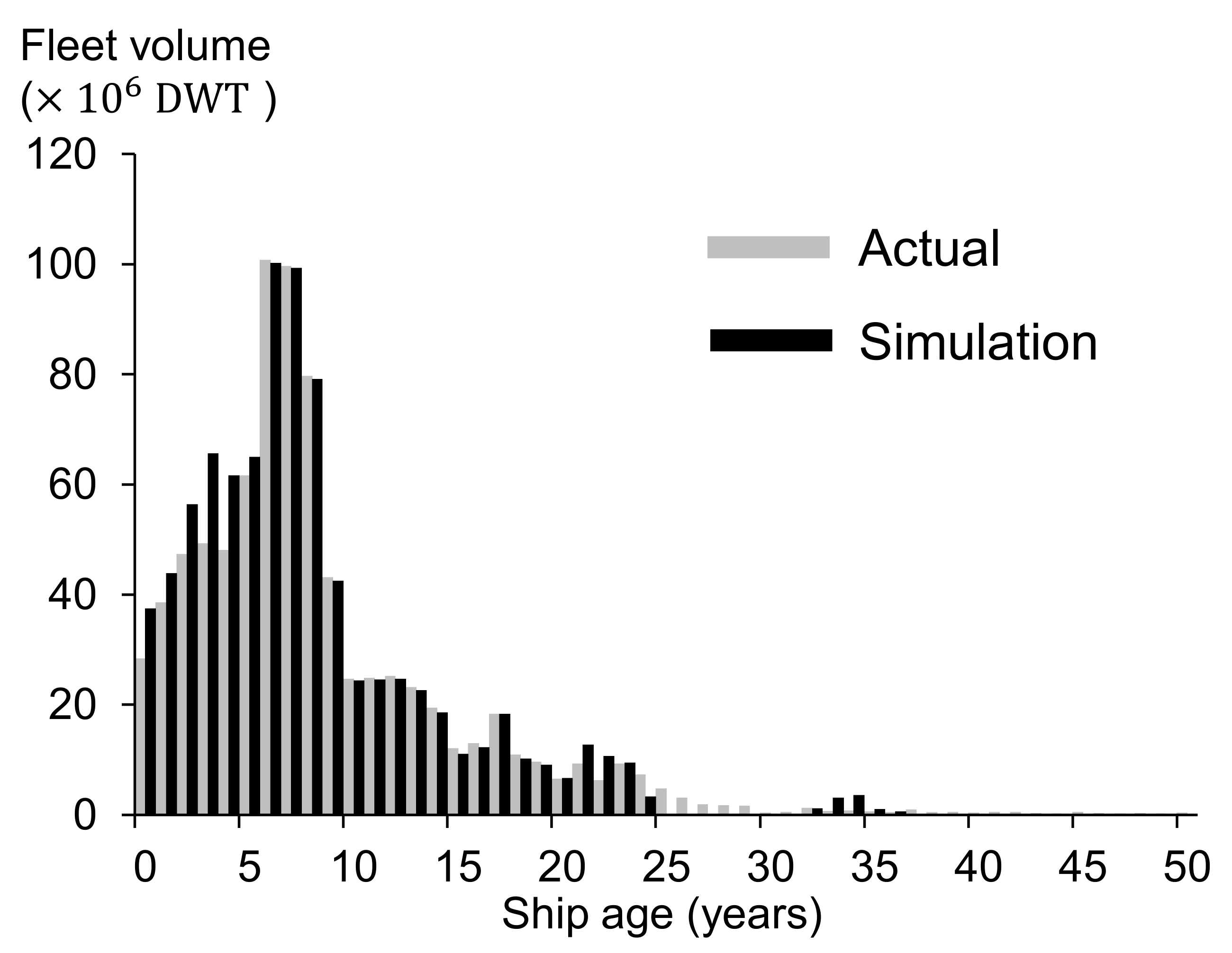
The scrap rate represents the probability of demolition for each age of ship based on the actual scrap data. As shown in Figure 5, the average scrap age becomes younger as the ship size increases. The average scrap age is 21.7 years for Capesize, 23.0 years for Panamax, 24.7 years for Handymax, and 27.3 years for Handysize. Using the scrap rate, we considered the actual conditions of scrap considering ship age. The ship composition is calculated using Equations (5)–(8):

$$D_t^i = f_2^i\left(E_t,S_t\right) \times V_t^i,$$

(5)

$$D_{a,t}^i = f_3^i\left(D_t^i\right),$$

(6)

$$S{d}_{a,t}^i = S{c}_{a,t}^i - D_{a,t}^i,$$

(7)

$$S{c}_{a,t+1}^i = S{d}_{a+1,t}^i + C_{0,t}^i,$$

(8)

where D is the amount of scrap (DWT), f₂ is each size of scrap model in Figure 4, E is ship running distance (miles), S is operating speed rate (-), V is fleet volume for each ship size (DWT), f₃ is the each scrap rate in Figure 5, Sd is ship composition deducted each age of scrap ships (DWT), Sc is ship composition (DWT), C is the amount of construction (DWT), a is the age of ships, i is the size of ships, and t is simulation time (months).

4. Model Validation

To confirm the validity of the modeled predictions of CO₂ emissions and ship composition, hindcast simulations were performed for the 2013 to 2018 period. The purpose of this validation is to confirm the validity of the newly developed model (i.e., the GHG emission prediction model and update of ship composition) in this study. The validity of the number of orders, amounts of scrap, and the other elements of sub-models in Figure 1 were confirmed in previous research [17,21]. The initial values are the input scenarios shown below.

• Input scenarios: January 2013 to December 2018

  (1)

  World GDP: (actual data)

  (2)

  Cargo transportation distance: (actual data)

  (3)

  Operating speed (actual data)

• Initial values: January 2013

  (1)

  Fleet volume: 6.80 × 10⁸ (DWT)

  (2)

  Order books: 1.40 × 10⁸ (DWT)

  (3)

  Construction capacity: 9.85 × 10⁶ (DWT)

  (4)

  Ship amount under construction: 5.10 × 10⁷ (DWT).

The simulation results for CO₂ emissions are shown in

Table 4. Simulation results of CO₂ emissions from 2013 to 2018.

Year	2013	2014	2015	2016	2017	2018
Fourth IMO GHG Study (×106 tons)	177.7	177.3	184.2	192.0	198.4	193.4
This Study (×106 tons)	176.6	181.7	182.3	189.0	193.4	196.8
Error (%)	−0.6	+2.5	−1.0	−1.6	−2.5	+1.8

. From these results, CO₂ emissions were estimated within an error margin of ±2.5%. There is no large error, and CO₂ emissions can be predicted well.

The simulation results for the ship composition are shown in Figure 6. The ship composition in December 2018 can be reproduced from the results. From these results, the validity of the entire model was confirmed.

In the fourth IMO GHG study [4], detailed ship movement data (i.e., AIS data) and various other data were utilized to estimate recent CO₂ emissions. In this study, we developed a model that obtained results similar to IMO’s GHG study without the use of detailed ship movement data. In the proposed model, CO₂ emissions’ forecasting can be executed by setting the scenario for GDP and cargo transportation distance only. This is an advantage for forecasting CO₂ emissions under the proposed model.

5. Case Study

In this section, the influences of current and future GHG emission measure deployment scenarios are considered using the proposed model. Concretely, evaluation of current measures for GHG emission reduction, especially deceleration operation, transition to LNG fuel, and technological development to achieve EEDI regulation, is done in Section 5.1. In Section 5.2, we evaluate future measures for GHG emission reduction, especially the introduction of zero-emission ships. In Section 5.3, we evaluate the combination of current and future measures in GHG emission reduction. In Section 5.4, we consider the limitation of deceleration operation and the effectiveness of combining shipping and shipbuilding market models and GHG emission prediction models. In Section 5.5, we discuss the simulation results from Section 5.1, Section 5.2, Section 5.3 and Section 5.4.

5.1. Impact Assessment of Current Measures

5.1.1. Overview of Current Measures

The current measures are explained in this section.

(1)

Deceleration operation: This measure can suppress GHG emissions by reducing the main engine’s output to save fuel during voyages. The average operating speed for ships has reduced since 2008.

(2)

Transition to LNG fuel: LNG, which has the effect of reducing fuel consumption and the carbon content rate, is drawing attention as an alternative to heavy fuel oil (HFO). The carbon content rate (Cf in Equation (2)) is 3.114 (gCO₂/gfuel) in HFO and 2.750 (gCO₂/gfuel) in LNG. SFC in Equation (2) is 156 g/kWh in LNG. In HFO, SFC in Equation (2) is utilized in Table 3. These values are from the fourth IMO GHG study [4]. Carbon content rate (Cf) and SFC were lower in LNG fuel than in HFO fuel.

(3)

Technological development to achieve EEDI regulation: EEDI is the amount of CO₂ emissions when carrying 1 ton of cargo for 1 mile. By restricting this value, the fuel efficiency of ships is promoted and CO₂ emissions are reduced. As the percentage of ships in the fleet volume that has passed regulation value increases with each passing year, it is necessary to take a long-term perspective on impact assessment of the EEDI regulation. In this study, we assumed that the EEDI regulation will be achieved by technology development, such as reduction of hull resistance and improvement of propeller efficiency in HFO ships.

5.1.2. Scenario Settings

To evaluate current GHG reduction measures, simulations for 2013–2050 were conducted. The market conditions in 2013 were used as initial values, and the following scenarios for current measures were inputted:

(1)

World GDP: Actual values for 2013–2019 were used and 3.5% GDP growth from 2020 was assumed. This assumption was based on the average GDP growth rate from 1980 to 2019, obtained from the International Monetary Fund [26].

(2)

Cargo transportation distance: Actual values for 2013–2019 were used, and after 2020, the values were assumed to be constant.

(3)

Operating speed reduction: It is still unclear how much ships will slow down in the future shipping industry. In this study, the actual value was used for 2013–2019, and after 2020, it was assumed that the speed is linearly reduced until 2050, reaching the intensity of deceleration that achieves 40% deceleration in 2050. The influence of operating speed reduction on GHG emissions and the implication for the maritime market industry are discussed in Section 5.4.

(4)

Transition to LNG fuel: The balance of construction for HFO- versus LNG-fueled ships is shown in

Table 5. Percentage of construction volume of liquid natural gas (LNG)-fueled ships.

Year	–2019	2020–2029	2030–2039	2040–2050
Fleet scenario: LNG
HFO (%)	100	50	40	30
LNG (%)	0	50	60	70

. We assumed that the ratio of LNG-fueled ships to total construction is set at 50% in 2020–2029, 60% in 2030–2039, and 70% in 2040–2050. In actuality, the order books of LNG-fueled ships among all type of ships for 2020 were approximately 12.2% based on the Clarkson database [23], and HFO ships are still the main ordered ships. This scenario is different from actual trends.

(5)

Technological development to achieve EEDI regulation: We impose a 10% reduction of CO₂ emission efficiency in ships built after 2015, a 20% reduction in ships built after 2020, and 30% reduction in ships built after 2025 as compared with the 2013 EEDI regulation level. This scenario was based on the IMO resolution [27].

Table 6. Scenarios for energy efficiency design index (EEDI) efficiency improvement.

Year	EEDI Regulation	Reduction Relative to Baseline, Taking SFC into Account
After 2013	0%	−7.5%
After 2015	10%	2.5%
After 2020	20%	12.5%
After 2025	30%	22.5%

shows the impact of SFC on EEDI efficiency improvement. The effects of EEDI efficiency improvement on SFC parameters of the main engine are estimated in the third IMO GHG study [1], and we used this table in this study.

To evaluate these GHG reduction effects, the following evaluation criteria were established:

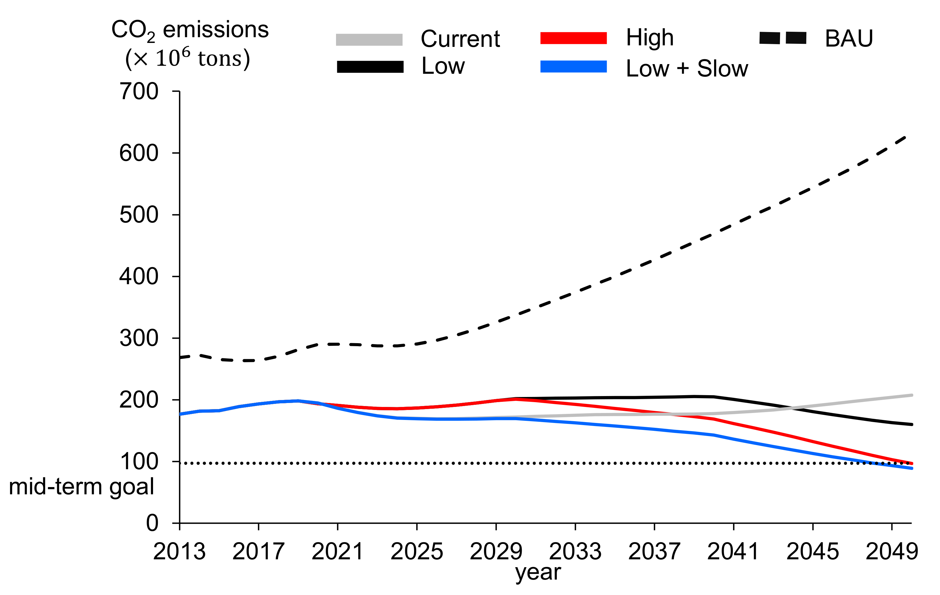
• Business as usual (BAU) lines: The base year for CO₂ emissions is set as 2008 based on the initial IMO strategy for reduction of GHG emissions from ships [22]. The BAU lines indicate that some GHG reduction measures have not been applied since 2008. The BAU lines are calculated using the model proposed in this study.
• Mid-term goal: In the initial strategy for reducing GHG emissions [22], the goal of halving GHG emissions by 2050 was decided based on 2008. Based on this strategy, a mid-term goal of 50% reduction of CO₂ emissions of bulk carriers by 2050 as compared with 2008 was set. CO₂ emissions of bulk carriers in 2008 were 194.0 × 10⁶ tons based on the third IMO GHG study [1]. Therefore, the mid-term goal is set at 97.0 × 10⁶ tons in this study. It should be noted that CO₂ emissions of bulk carriers were 193.4 × 10⁶ tons in 2018. Comparing the CO₂ emissions in 2018 and 2008, no significant change was found.

These evaluation criteria are original to this study and differ from the existing IMO criteria. For example, the BAU lines of total CO₂ emissions considering several types of ships (for example, bulk carriers, tankers, container ships, general cargo ships, and LNG ships, among others) were shown in the fourth IMO GHG study [4]. However, the BAU lines in the IMO’s study were considered as the influence of GHG emission measures, and the evaluation of the CO₂ reduction effect of each measure is difficult using the IMO’s BAU lines. Therefore, the BAU lines in this study were simulated using the proposed model and utilized as a baseline to evaluate the reduction in CO₂ emissions quantitatively by several emission measures. The BAU lines simulated using the proposed model are different from those in the IMO’s study.

5.1.3. Simulation Results for Current Measures

In this simulation, we analyzed the CO₂ emission reduction effect of the current measures alone. The simulation results of CO₂ emissions considering operating speed reduction, the transition to LNG fuel, and technological development to achieve EEDI regulation are shown in Figure 7. In the case of the BAU scenario, CO₂ emissions will increase approximately 3.3 times by 2050 with respect to 2008 CO₂ emissions. This is because the influence of HFO ships increases with an increase in sea cargo movement. In the case of operating speed reduction, CO₂ emissions decrease by 56.1% with respect to BAU lines by 2050. In the case of EEDI, CO₂ emissions decrease by 24.3% with respect to BAU lines by 2050. In the case of transition to LNG fuel, CO₂ emissions decrease by 14.6% with respect to BAU lines by 2050. As a result, operating speed reduction more effectively reduces emissions compared with EEDI efficiency improvement and the transition to LNG fuel. However, it is difficult to achieve the mid-term goals of 50% decrease with respect to 2008 CO₂ emissions using a single measure alone; instead, it is necessary to combine measures. Based on these results, we considered deceleration of operating speed, transition to LNG fuel, and technological development to achieve EEDI regulation.

5.2. Impact Assessment of Future Measures

5.2.1. Scenario Settings

To examine measures to reduce GHG emissions that achieve the mid-term goal, one new measure, the introduction of zero-emission ships, was introduced and evaluated for after 2030. The initial values are the same as those in Section 5.1.2. The additional measures incorporated are as follows:

• Introduction of zero-emission ships: Zero-emission ships use hydrogen (H₂) fuel, ammonia (NH₃) fuel, or other alternatives. By using these fuels, GHG emissions from shipping become zero and significant reductions of GHG emissions are realized compared with current measures.

Two types of scenarios to introduce zero-emission ships (low case and high case) are constructed and assumed to change the fleet composition if implemented. The scenarios are listed in

Table 7. Percentage of construction volume of alternative fuels. HFO, heavy fuel oil; LNG, liquid natural gas.

Year	–2019	2020–2029	2030–2039	2040–2050
Fleet Scenario: Low
HFO (%)	100	20	10	0
LNG (%)	0	80	60	30
Zero-Emission Fuel (%)	0	0	30	70
Fleet Scenario: High
HFO (%)	100	20	0	0
LNG (%)	0	80	40	10
Zero-Emission Fuel (%)	0	0	60	90

. We assume that only HFO fuel ships are constructed until 2019. After 2020, the construction of LNG-fueled ships begins. After 2030, the construction of zero-emission ships begins. Each number shows the ratio of fuel ship types to be built. This percentage applies to the ships that are constructed, and the ships are added to the fleet composition. The scenarios of GDP and cargo transportation distance scenarios follow in Section 5.1.2.

5.2.2. Evaluation Results with Future Measures

In this simulation, we analyzed the CO₂ emission reduction effect of the introduction of zero-emission ships alone. The simulation results of CO₂ emissions considering introduction of zero-emission ships are shown in Figure 8. The reduction effect of the introduction of zero-emissions ships is considerably larger than that of other measures; CO₂ emissions decrease by 57.9% in the low scenario with respect to BAU lines by 2050 and by 75.4% in the high scenario with respect to BAU lines by 2050, because the ratio of zero-emission ships to fleet volume directly contributes to the reduction of CO₂ emissions. If all ships are replaced by zero-emission ships, CO₂ emissions will be fully eliminated; however, replacing all ships would be difficult given the immature state of zero-emission technology, and thus introduction of zero-emission ships fluctuates greatly depending on the (projected) status of technology development.

5.3. Impact Assessment of Combination of Current and Future Measures

5.3.1. Scenario Settings

The simulation combines current measures (operating speed reduction, technological development to achieve EEDI regulation, and transition to LNG fuel) and future measures (introduction of zero-emission ships). The purpose of this simulation is to quantitatively grasp the CO₂ reduction effect when current and future measures are combined. In addition, we consider the scenarios to satisfy the mid-term goal for 2050. The following assumptions were used in this simulation.

• Technological development to achieve EEDI regulation is applied to HFO and LNG-fueled ships.
• Reduction in operating speed applies to HFO and LNG-fueled ships; zero-emission ships are not the target of operating speed reduction, which thus does not occur for them. This is because zero-emission ships are more efficient with regards to CO₂ emissions compared with HFO and LNG-fueled ships. Additionally, LNG-fueled ships are more efficient in terms of CO₂ emissions than HFO fuel ships. Therefore, the speed of LNG-fueled ships is 10% faster than that of HFO ships. This assumption is based on the concepts of energy efficiency existing ship index (EEXI) regulation [28].

In this simulation, we consider the four types of cases shown in

Table 8. The scenario for simulation of combination of current and future measures. EEDI, energy efficiency design index.

Scenario Name	Fleet Scenario	Operating Speed Deceleration Scenario	Technological Development to Achieve EEDI Regulation	LNG Fuel	Zero-Emission Ships
Current	LNG (Table 5)	40% deceleration in 2050 (Linearly reduce)	◯	◯	N/A
Low	Low (Table 7)	Constant	◯	◯	◯
High	High (Table 7)	Constant	◯	◯	◯
Low + Slow	Low (Table 7)	40% deceleration in 2050 (Linearly reduce)	◯	◯	◯

◯: Applicable, N/A: Not applicable.

. The scenario of GDP and cargo transportation distance is the scenario in Section 5.1.2. The operating speed reduction was set to reach 40% deceleration in 2050 based on HFO fuel ships. In the low and high scenarios, the deceleration rate is set to 17% and is constant after 2020.

5.3.2. Evaluation Results for Combination of Current and Future Measures

The simulation results of CO₂ emissions for the combination of current and future measures are shown in Figure 9. In the current scenario, CO₂ emissions in 2050 are 207.3 × 10⁶ tons. On the other hand, in the case where only the 40% operating speed reduction measure is applied, the CO₂ emission amount becomes 277.6 × 10⁶ tons as of 2050. Compared with these results, CO₂ emissions are thus reduced by 70.3 × 10⁶ tons by EEDI efficiency improvement and transition to LNG fuel. However, it is difficult to achieve mid-term goals by 2050. From these results, it is found that the introduction of zero-emission ships is necessary to achieve mid-term goals.

In the case of low scenarios, if zero-emission measures are promoted after 2030 in addition to the current measures, it is difficult to achieve the mid-term goal by 2050; conversely, in high scenarios, the 2050 goal can be achieved. Similarly, in the low + slow scenarios, it is possible to achieve mid-term goals. Therefore, it is necessary to consider the transition to LNG fuel, introduction of zero emissions ships, deceleration operation, and technological development to achieve EEDI regulation from a long-term perspective.

The simulation scenario is set such that LNG fuel will be introduced from 2020, and a zero-emission ship is introduced from 2030. This scenario is extremely difficult to realize in relation to reality. Based on the above, to promote GHG reduction, it is necessary not only to promote the development of zero-emission ships, but also to implement additional GHG emission schemes such as market-based measures.

From the results, it can be seen that the influence of the combination of all measures on CO₂ emissions was considered.

5.4. Limitation of Operating Speed Reduction

It is clear that the ship operating speed reduction is effective in CO₂ emissions reduction from the results in Section 5.1.3. However, if excessive deceleration operation is performed, the required fleet quantity will increase sharply. In this simulation, the limit of deceleration is considered using the proposed model. The scenario of GDP and cargo transportation distance is the scenario of Section 5.1.2, and the cases of deceleration operation are four cases of 20%, 40%, 50%, and 70%.

The simulation results of CO₂ emissions considering deceleration operation are shown in Figure 10. In the case of 20%, 40%, and 50% deceleration, CO₂ emissions decrease as the ship speed decreases. In the case of a 70% deceleration, CO₂ emissions decrease progress until 2038. However, CO₂ emissions increased from 2039 because of an increase in shipbuilding orders.

The results under the impact of increases in fleet volume and shipbuilding orders are shown in Figure 11. Both fleet volume and orders increase as the deceleration strength increases. This is the influence of the correction of the order prediction model (Section 3.4). By increasing the operating speed decelerations, it is expected that ship orders will also increase, and the shipbuilding industry can benefit. Especially in the case of a 70% deceleration, orders increase rapidly and fluctuate from 2033, and the fleet volume increases rapidly after 2039. This rapid increase in ship orders is caused by a significant shortage of ship capacity due to rapid deceleration. Although 70% had excessive deceleration, CO₂ emissions increased gradually as the fleet increased. The engine load factor is very small (less than 5%); therefore, CO₂ emissions increase gradually compared with the fleet increase. The fleet volume becomes insufficient, and marine transportation has failed to meet demand because of a significant shortage of fleet volume in 70% deceleration, and 70% deceleration is difficult from a maritime transportation perspective. From these results, it was found that the limitation of deceleration in ship operations was approximately 50%.

We also showed that, by combining such a model of GHG emissions with a model of the shipping and shipbuilding market, the effect of reducing GHG emissions can be analyzed based on dynamic changes in the market.

5.5. Discussion

In Section 5.1, we conducted a quantitative evaluation of the current measures for CO₂ emission reduction, especially deceleration operation, transition to LNG fuel, and technological development, to achieve EEDI regulation. The result suggests that the deceleration operation had the highest CO₂ reduction effect, followed by technological development to achieve EEDI regulation and transition to LNG fuel. In particular, the CO₂ emission reduction effect by the deceleration operation considers change in orders and scrap due to the operating speed reduction; few or no evaluations that consider the maritime market aspect have been conducted in previous studies. By modeling the relationship between operation speed and number of orders and between operation speed and amount of scrap, our model enables this consideration.

In Section 5.2, we evaluated the introduction of zero-emission ships for CO₂ emission reduction. The result demonstrates that our model can forecast the impact of the future introduction of zero-emission ships, considering the transition from current ships. In the simulation, we assumed two scenarios of the introduction of zero-emission ships and evaluated the amount of CO₂ emission reduction by the introduction. However, American Bureau of Shipping [29] has reported that zero-emission ships are still at the research stage, and the scenario for their introduction has not become clear yet. The introduction of zero-emission ships greatly depends on the projected status of technology development, thus it is necessary to carefully consider what scenarios should be evaluated.

In Section 5.3, we evaluated the combination of current and future measures for CO₂ emission reduction. In the simulation, EEXI measures for existing ships are also taken into consideration. The result shows that it is difficult to achieve the IMO goals for 2050 by combining only current measures. Additionally, the result shows that the target for 2050 can be achieved in the “high“ scenario, which introduces many zero-emission ships, or the “low + slow” scenario, which introduces zero-emission ships and deceleration operation. In the “high” scenario, zero-emission ships account for 60% of ships constructed from 2030; achieving this is considered difficult at the present stage of development of zero-emission ships. The “low + slow“ scenario is considered to be more realistic from the perspective of achieving IMO goals for 2050; however, the amount of LNG-fueled ships on order books for all ship types is only approximately 12.2% as of 2020 [23], which is still lower than the assumption of the “low + slow” scenario. Based on these considerations, it is necessary not only to promote the development of zero-emission ships, but also to implement additional GHG emission schemes such as market-based measures.

In the fourth IMO GHG study [4], future CO₂ emissions are predicted. It is reported that CO₂ emissions in 2050 will be approximately 90–130% compared with 2008 owing to deceleration operation, EEDI efficiency improvement, improvement of operation efficiency, and so on. This result can be interpreted to show that additional measures, such as the introduction of zero-emission ships and market-based measures, are required to achieve the 2050 GHG emission target. The “current” scenario in Figure 9 confirms the effectiveness of the current measures and shows that the case where only current measures are combined makes it difficult to achieve the 2050 GHG emission target. The results of the forth IMO study and the simulation results in this study are qualitatively consistent. This paper is novel in that we considered multiple scenarios—“high” and “low + slow”—and the simulation results suggest some example roadmaps for the implementation of the IMO’s GHG reduction strategy. Those examples can serve as reference data to discuss the future development of decarbonized shipping, and this is one of the important contributions of this paper.

In Section 5.4, we considered the limitation of deceleration operation and the effectiveness of combining shipping and shipbuilding market models and GHG emission prediction models. In this simulation, we analyzed the limit of deceleration operation from the maritime market perspective and showed that the limit of deceleration operation is approximately 50%. Previous studies cannot consider this limitation because their models do not combine GHG emission prediction and maritime market models. This case suggests the importance of considering the maritime market when evaluating the effect of deceleration, and this consideration is also part of the novelty of our model.

The simulations in Section 5.1, Section 5.2, Section 5.3 and Section 5.4 demonstrate that our model can analyze dynamics in the maritime market when GHG emission measures are implemented. The results can be used for the establishment of international rules such as IMO rules and for policy making in maritime governance. Specifically, it will be possible to study a scenario with the introduction of zero-emission ships and to analyze market fluctuations due to regulations on existing ships such as EEXI regulation [28].

6. Conclusions

In this study, a model to consider GHG emission scenarios for the maritime transportation sector was developed using SD. Using this model, the influence of several GHG emissions reduction scenarios was examined. Additionally, several simulations were executed using the proposed model, and we evaluated the impacts of several measures on GHG emissions. Then, we built a theoretical framework to develop a model that comprehensively evaluates the impact of GHG reduction measures in the maritime market. The conclusions can be summarized as follows:

• To estimate GHG emissions, a GHG emissions prediction model was developed and the scrap model was improved. Additionally, the GHG emissions prediction model was integrated into shipping and shipbuilding market models, and a model to consider GHG reduction measures was developed.
• To confirm the validity of the evaluation model for GHG reduction measures, simulations from 2013 to 2018 were conducted. The model validity was confirmed quantitatively.
• The GHG emission reduction effect by current measures and future measures alone was evaluated. Additionally, the impact and effectiveness of combining current measures and future measures were evaluated.
• The comprehensive scenarios to achieve IMO GHG emission goals were discussed considering current and future GHG reduction measures. From this simulation result, it was found that, in order to achieve the target of 2050, it is necessary to develop a zero-emission ship in addition to the current measures.
• We focused on the deceleration of operating speed, the influence of which on shipping and shipbuilding markets was evaluated. Concretely, the limitation of deceleration was considered from the maritime market perspective. This simulation result suggests that the limitation of ship operating speed reduction is approximately 50% from the maritime market perspective.

However, on the other hand, the developed model is still insufficient for cost calculation. Concretely, measures to reduce GHG emissions affect ship operating costs and ship prices. However, the influences of ship operating costs and ship prices have not been considered in this study. In future work, we will expand the model to simulate these items, and develop a model to consider optimal scenarios in terms of the balance between maritime market and GHG emissions. Additionally, the proposed model predicts the amount of sea cargo movement using GDP and cargo transportation distance. However, it is difficult to accurately predict these values because of the uncertainties involved. In future work, we are considering how to handle these uncertainties. The sophistication of the shipping and shipbuilding market model is also an issue for future work. In recent years, it has become possible to grasp the ship movement in real time by development of AIS and to obtain detailed cargo flow volume of dry bulk cargo based on ship movement [30]. By using such ship movement data, it is expected that sophisticated cargo transportation volume data will be achievable and the shipping and shipbuilding market model in this study will improve as a predictive tool.

References

1. Smith, T.W.P.; Jalkanen, J.P.; Anderson, B.A.; Corbett, J.J.; Faber, J.; Hanayama, S.; O’Keeffe, E.; Parker, S.; Johansson, L.; Aldous, L.; et al. Third IMO Greenhouse Gas Study 2014; International Maritime Organization: London, UK, 2015. [Google Scholar]
2. Komiyama, R.; Suzuki, K.; Nagatomi, Y.; Matsuo, Y.; Suehiro, S. Analysis of Japan’s energy demand and supply to 2050 through integrated energy-economic model. J. Jpn. Soc. Energy Resour. 2012, 33, 34–43. (In Japanese) [Google Scholar]
3. Holz, C.; Siegel, L.; Johnston, E.; Jones, A.; Sterman, J. Ratcheting ambition to limit warming to 1.5 °C: Trade-offs between emission reductions and carbon dioxide removal. Environ. Res. Lett. 2018, 13, 064028. [Google Scholar] [CrossRef] [Green Version]
4. IMO: Fourth IMO GHG Study 2020, IMO MEPC 75/7/15. 2020. Available online: https://docs.imo.org/ (accessed on 6 August 2020).
5. Faber, J.; Markowska, A.; Eyring, V.; Cionni, I.; Selstad, E. A Global Maritime Emissions Trading System—Design and Impacts on the Shipping Sector, Countries and Regions; CE Delft: Delft, The Netherlands, 2010. [Google Scholar]
6. Lindstad, E.; Rialland, A. LNG and cruise ships, an easy way to fulfil regulations—versus the need for reducing GHG emissions. Sustainability 2020, 12, 2080. [Google Scholar] [CrossRef] [Green Version]
7. Rehmatulla, N.; Calleya, J.; Smith, T. The implementation of technical energy efficiency and CO2 emission reduction measures in shipping. Ocean Eng. 2017, 139, 184–197. [Google Scholar] [CrossRef]
8. Kobayashi, M.; Hashiguchi, Y.; Sawada, N. Actual status of slow-down operation: Challenges, countermeasures, and results of slow-down operation. J. Jpn. Inst. Mar. Eng. 2014, 49, 74–80. (In Japanese) [Google Scholar] [CrossRef] [Green Version]
9. Smith, T.W.P. Technical energy efficiency, its interaction with optimal operating speeds and the implications for the management of shipping’s carbon emissions. Carbon Manag. 2012, 3, 589–600. [Google Scholar] [CrossRef]
10. Nielsen, K.S.; Kristensen, N.E.; Bastiansen, E.; Skytte, P. Forecasting the market for ships. Long Range Plan. 1982, 15, 70–75. [Google Scholar] [CrossRef]
11. Sakalayen, Q.M.H.; Duru, O.; Hirata, E. An econophysics approach to forecast bulk shipbuilding orderbook: an application of Newton’s law of gravitation. Marit. Bus. Rev. 2020. [Google Scholar] [CrossRef]
12. Gourdon, K. An Analysis of Market-Distorting Factors in Shipbuilding: The Role of Government interventions, OECD Science, Technology and Industry Policy Papers; OECD Publishing: Paris, France, 2019; Volume 67. [Google Scholar]
13. Shin, J.; Lim, Y.-M. An empirical model of changing global competition in the shipbuilding industry. Marit. Policy Manag. 2014, 41, 515–527. [Google Scholar] [CrossRef]
14. Taylor, A.J. The dynamics of supply and demand in shipping. Dynamica 1975, 2, 62–71. [Google Scholar]
15. Japan Maritime Research Institute SD Study Group. SD model of maritime transportation and shipbuilding. Jpn. Marit. Res. Inst. Bull. 1978, 142. (In Japanese) [Google Scholar]
16. Engelen, S.; Meersman, H.; Eddy, V.D.V. Using system dynamics in maritime economics: An endogenous decision model for ship owners in the dry bulk sector. Marit. Policy Manag. 2006, 33, 141–158. [Google Scholar] [CrossRef]
17. Wada, Y.; Hamada, K.; Hirata, N.; Seki, K.; Yamada, S. A system dynamics model for shipbuilding demand forecasting. J. Mar. Sci. Technol. 2018, 23, 236–252. [Google Scholar] [CrossRef]
18. Forrester, J.W. Industrial Dynamics; MIT Press: Cambridge, MA, USA, 1961. [Google Scholar]
19. Sterman, J. Business Dynamics: Systems Thinking and Modeling for a Complex World; Irwin Professional Publishing: Burr Ridge, IL, USA, 2000. [Google Scholar]
20. Sterman, J.; Fiddaman, T.; Franck, T.R.; Jones, A.; McCauley, S.; Rice, P.; Sawin, E.; Siegel, L. Climate interactive: The C-ROADS climate policy model. Syst. Dyn. Rev. 2012, 28, 295–305. [Google Scholar] [CrossRef] [Green Version]
21. Wada, Y.; Hamada, K.; Hirata, N. A Study on the Improvement and Application of System Dynamics Model for Demand Forecasting of Ships. In Proceedings of the International Conference on Computer Applications in Shipbuilding, 1, Singapore, 26–28 September 2017; pp. 51–60. [Google Scholar]
22. IMO MEPC72. Resolution MEPC.304(72). Initial IMO Strategy on Reduction of GHG Emissions from Ships. 2018. Available online: https://wwwcdn.imo.org/localresources/en/KnowledgeCentre/IndexofIMOResolutions/MEPCDocuments/MEPC.304(72).pdf (accessed on 21 January 2021).
23. Clarksons Shipping Intelligence Network. Available online: http://www.clarksons.net (accessed on 6 February 2021).
24. Sea-Web Ships. Available online: https://maritime.ihs.com/Account2/Index (accessed on 8 December 2019).
25. Buhaug, Ø.; Corbett, J.J.; Endresen, Ø.; Eyring, V.; Faber, J.; Hanayama, S.; Lee, D.S.; Lee, D.; Lindstad, H.; Markowska, A.Z.; et al. Second IMO GHG Study 2009; International Maritime Organization (IMO): London, UK, 2009. [Google Scholar]
26. International Monetary Fund. Available online: https://www.imf.org/external/datamapper/NGDP_RPCH@WEO/WEOWORLD (accessed on 17 January 2021).
27. IMO MEPC 62/24/Add.1, ANNEX 19 RESOLUTION MEPC.203(62), 2011. Available online: https://wwwcdn.imo.org/localresources/en/OurWork/Environment/Documents/Technical%20and%20Operational%20Measures/Resolution%20MEPC.203(62).pdf (accessed on 7 December 2020).
28. Japan Ship Technology Research Association; Ministry of Land, Infrastructure, Transport and Tourism. Roadmap to Zero Emission from International Shipping; Ministry of Land, Infrastructure, Transport and Tourism: Tokyo, Japan, 2020.
29. American Bureau of Shipping (ABS). Ammonia as Marine Fuel; ABS Sustainability Whitepaper; 2020. Available online: https://absinfo.eagle.org/acton/fs/blocks/showLandingPage/a/16130/p/p-0227/t/page/fm/0 (accessed on 7 December 2020).
30. Kanamoto, K.; Murong, L.; Nakashima, M.; Shibasaki, R. Can maritime big data be applied to shipping industry analysis? Focussing on commodities and vessel sizes of dry bulk carriers. Marit. Econ. Logist. 2020. [Google Scholar] [CrossRef]
Figure 1. Evaluation model for greenhouse gas (GHG) reduction measures. GDP, gross domestic product.
Sustainability 13 02760 g001
Figure 2. The order prediction model.
Sustainability 13 02760 g002
Figure 3. Relation between operating speed reduction scenario and order prediction model.
Sustainability 13 02760 g003
Figure 4. Scrap model for each size of ship. (a) Scrap model for Capesize; (b) Scrap model for Panamax; (c) Scrap model for Handymax; (d) Scrap model for Handysize.
Sustainability 13 02760 g004
Figure 5. Scrap rate by ship age. (a) Scrap rate for Capesize; (b) Scrap rate for Panamax; (c) Scrap rate for Handymax; (d) Scrap rate for Handysize.
Sustainability 13 02760 g005
Figure 6. Composition of observed and simulated ship ages in 2018.
Sustainability 13 02760 g006
Figure 7. Simulation results of CO2 emissions considering current measures. LNG, liquid natural gas; EEDI, energy efficiency design index; BAU, business as usual.
Sustainability 13 02760 g007
Figure 8. Simulation results of CO2 emissions considering the introduction of zero-emission ships.
Sustainability 13 02760 g008
Figure 9. Simulation results of CO2 emissions for the combination of current and future measures.
Sustainability 13 02760 g009
Figure 10. Simulation results of CO2 emissions considering deceleration operation.
Sustainability 13 02760 g010
Figure 11. Simulation results for fleet volume and shipbuilding orders.
Sustainability 13 02760 g011