Abstract
This study assesses how the initial economic context of a country functions as a factor in the progression of the SARS-CoV-2 pandemic. To do so, we analyze Chile during the first wave of the pandemic. Chile is a developing country that suffered an unprecedented social disturbance (the Social Outbreak) that deteriorated economic activity and increased unemployment just months before the pandemic begun. We empirically test the hypothesis that the previous deterioration in the labor market, as an indicator of economic deterioration at the beginning of the pandemic, impacted the infection rate. Our results show a positive and significant relationship between unemployment prior to the pandemic at a provincial level and the number of individuals infected by SARS-CoV-2. All in all, we provide evidence that the initial social and socioeconomic conditions of each territory must be considered in the design of any policy aimed at minimizing the effects of the pandemic.
1. Introduction
The objective of this study is to analyze how labor market conditions prior to the severe acute respiratory syndrome coronavirus 2 (SARS-CoV-2) pandemic might have an impact on the infection rate, allowing us to understand the heterogeneous effect of the disease over a territory, in that some areas, albeit under the same disease control policies, might have a better response in fighting it. To achieve this objective, we analyze Chile, the South American country with the highest rate of infection per 100,000 inhabitants.
South America became the epicenter of the SARS-CoV-2 pandemic in a third wave after it passed through Asia, Europe and the United States, and it threatens the region with one of its greatest crises since the “lost decade” of the 1980s [1] (Table A1 in Appendix A). The pandemic began its spread in Chile only five months after an unprecedented social disturbance (the Social Outbreak) that resulted in significant institutional uncertainty and negatively affected growth and employment. The pandemic has deepened the macroeconomic and social deterioration of the country [2] and, with it, the loss of household income, which has limited the effectiveness of measures designed to contain the spread of the disease and poses a debate about what the most appropriate measures to contain it are.
The case of Chile is particularly relevant because it involves a social, political and economic crisis resulting from the Social Outbreak as well as the effects of the pandemic. The evolution of the pandemic in Chile has also been peculiar. The first imported cases, occurring from the second half of March to May, were concentrated in the wealthiest municipalities of the country and progressed at a relatively slow pace. However, the rate of infection increased rapidly in May (Figure A1 in Appendix A) as the pandemic spread towards the poorest municipalities. By the end of July, Chile had the highest rate of infection per 100,000 inhabitants among the fifteen countries with the highest number of total cases (Table 1).

Table 1.
Top 15 countries with the highest number of infected individuals and the infection rates per 100,000 inhabitants on 31 July 2020.
Identifying elements of the progression of the disease is crucial to limiting its advance and to designing appropriate policies beyond quarantines to safely recuperate economic activity in Chile and in other developing countries, all of which may be facing similar conditions, not only now but also in the future.
2. Economic Conditions in Developing Countries and the Evolution of the Pandemic: The Case of Chile
This section first analyzes the relevance of initial economic conditions for understanding the evolution of the pandemic. Next, we examine Chile’s economic and political context during the months prior to (when a profound social disturbance occurred, nearly paralyzing the country) and during the pandemic, as we attempt to understand how a country’s characteristic economic conditions can have a direct impact on infection rate (per 100,000 inhabitants).
2.1. Initial Economic Conditions and the Evolution of the Pandemic
The pandemic, which was first identified in China in late 2019 and rapidly became a global threat, poses an unprecedented public policy challenge. The vertiginous transmission of the disease at a global level and the exponential growth in the number of those infected in nearly every country in the world pose enormous difficulties for health systems in each territory (be it a country, region or municipality) affected. This has meant that confinement and social distancing measures have become necessary in order to facilitate disease control, to prevent the collapse of health systems [3] and, most importantly, to save lives.
However, the opportunity cost associated with these measures has also been significant, primarily the paralysis of economic activity (except for those sectors that supply products and services of basic necessity) and the subsequent loss of income and jobs. The economic impact of the pandemic in 2020 included a projected decrease in global GDP of between 4.9% and 5.5% [4,5] and a significant increase in poverty, particularly in developing economies [6].
The need to develop policies that simultaneously minimize the loss of life and the negative impact on economic growth of the measures adopted has been a challenge for the governments of the affected countries [7]. Various studies have rapidly emerged to support the development and improvement of public policies aimed at limiting the infections rate and reducing the economic collateral effects. Of special interest are the studies [7,8,9], which propose the definition of an “optimal lockdown policy” aimed at minimizing both the health and economic impacts of the pandemic. These proposals, however, do not consider how a country’s initial economic conditions and social context influence the pandemic response, potentially handicapping the design and effectiveness of policies focused on the idea of confinement.
In the work of [10], the authors find that the mortality rate of the 1918 Spanish flu had a negative correlation (of −0.43) with the log of a country’s real per capita GDP in 1913 for the 42 economies considered in the study. This result could reflect that economies with a higher per capita income at the beginning of the pandemic also had better health systems to deal with it, which would provide greater guarantees regarding control of the disease and ultimately the survival of the population. This evidence, although not studied in depth in that study, could be indicative of the importance of a country’s economic context on infections rate. This is fundamental for developing countries, given that their macroeconomic and social conditions may be more heavily affected by the crisis caused by the pandemic. According to this logic, social and economic context is essential to designing a set of policies that are thus adapted to each country, rather than a standardized one-size-fits-all approach that is expected to have the same effectiveness in each and every one of the countries to which it is applied.
Confinement has been the most recurrent policy used to limit the spread of the disease and Chile is no exception. Between late March and the end of June, the period of the first wave of the disease in the country, about 60% of the population (approximately 11.8 million people) was under quarantine. To guarantee its effectiveness, confinement has been combined with income maintenance policies, aimed primarily at those households which have been negatively affected, either due to a reduction in working hours or the loss of employment. The combination of confinement and income maintenance policies seeks to reduce mobility and with it, the number of new infections.
However, these types of measures have proven difficult to apply in developing economies due to the inferior endowment of public resources available to face the pandemic, lower incomes (largely due to worse working conditions and high levels of informality) and lower levels of savings [11]. As a result, “staying at home is not a viable option, and not working comes at the expense of food and other necessities” [12] (p. 5). These economies also have less-developed production models and therefore have less capacity to incorporate social isolation policies alongside productive activity, due to a lower incorporation of information and communication technologies [13]. This limits the development of activities such as remote work and, therefore, the ability to work without needing to be physically present in a workplace. This situation increases the impact of the pandemic on the household income level and reinforces the importance of policies to cover lost income in order to prevent further infections [11].
2.2. The Chilean Economic Conditions: The Effect of the Social Outbreak and the Pandemic
Chile is an emerging economy which has experienced important economic development over the last three decades (1990–2019), its GDP per capita (GDP pc) increasing from USD $4511 pc in 1990 to USD $25,155 pc in 2019 (Purchasing Power Parities, current international USD, data from the World Development Indicators database). This growth is largely due to the exploitation and export of raw materials, particularly copper, for which Chile represents 16% of global production (COCHILCO database). In addition, between 2003 and 2011, the country experienced a sustained increase in the market price of the minerals extracted. The Chilean labor market was directly affected by this positive business cycle, adding approximately 1,000,000 new jobs, which helped in raising the income level and reducing the poverty level during the first decade of the 21st century [14].
Despite this economic development, Chile stands out for its high level of socioeconomic inequality. Wage inequality is one of the highest among OECD members and social mobility is very limited [15]. These features, coupled with the end of the mineral super cycle and the subsequent labor market deterioration [16], are all factors in understanding the unprecedented social disturbance that began in October of 2019.
The context in which Chile entered the pandemic is crucial to understanding how the previous economic deterioration limited the effectiveness of the containment measures applied thus far. On 18 October 2019, a series of mass protests began in the capital city of Santiago and quickly spread throughout the country, eventually paralyzing the economy. The economic result of the first three months of the social disturbance was a GDP contraction close to 2.5%, a figure estimated for the fourth quarter of 2019 [17]. The consequences on the labor market were also significant. Between the mobile quarters of November 2019–January 2020 and January–March 2020 (data from the Chilean National Employment Survey (ENE)), more than 175,000 jobs were lost (decreasing employment by 1.9%), and unemployment increased by 69,600 (9.5%). Approximately 427,000 people from outside the labor force were unable to find employment as a consequence of the Social Outbreak, a figure which includes those that declared that they were available to work or those that were unsuccessful in finding employment. This represents an increase of 36% during the quarters considered. If we incorporate this group into the labor supply (as they are technically unemployed) the unemployment rate in the January–March 2020 quarter reached 20.2%, more than doubling the official unemployment rate in that quarter, which was 9.8%. Chile therefore entered the pandemic in an incredibly complicated socioeconomic situation.
The measures adopted by the government to alleviate the impact of SARS-CoV-2 were as follows. On March 18, the government declared a state of national emergency. The first quarantines in Chile started in Easter Island on March 20 and in various municipalities of Santiago on March 26. On April 1, the Employment Protection Law was enacted, which allowed employers affected by the pandemic to reduce working hours or suspend employment contracts without dismissing their workers, allowing them to receive the benefits from unemployment insurance. However, these benefits were designed to decrease over time (70% of salary in the first month, 55% in the second, 45% in the third and 40% from the fourth month on).
In May 2020, the Chilean government decided to enact the Emergency Family Income (IFE) law in order to sustain the consumption capacity of the most vulnerable households, estimated at about 4.9 million people. This proposal was criticized from the political sphere for being insufficient with regard to the amount defined for the three months for which it was planned. The government defended the amount, arguing that it was likely to need more financial resources at a later date in order to respond to the economic impact of the pandemic and given the uncertainty regarding an end date. Additionally, at the end of May, 2.5 million food boxes were delivered to the most vulnerable families, prioritizing those with older adults, risk groups and those municipalities in quarantine. In June, the IFE was modified (IFE2), raising the amount by approximately 54% compared to the payment made in the first month, as well as the number of beneficiaries (reaching a total of 5.6 million people).
These initial measures were not enough to sufficiently reduce the mobility of the population or curb the total number of SARS-CoV-2 infections. In June, Chile had one of the highest rates of infection per 100,000 inhabitants in the world. A household survey carried out in the Metropolitan Region of Santiago that month by [18] showed that only 57% of the most vulnerable households had received some type of help from local municipalities or the central government. Ninety percent of this group viewed the monetary contribution as insufficient and 69% also viewed the food boxes as insufficient, both being factors in their ability to comply with the confinement policy. Members of the most vulnerable households had to leave their homes to work in a greater proportion (40% of the total) well above groups with a higher income (25%).
This situation of insufficient measures led to the emergence of a broad political debate that culminated in the enactment of a law authorizing the withdrawal of 10% of an individual’s pension funds. The law was passed with broad support in both houses of Congress in July and was supported by both the opposition and members of parties aligned with the Government. It was broadly agreed that the measures applied thus far had been insufficient in sustaining consumption capacity, particularly that of the middle class. Finally, a “middle class” stimulus grant of CLP $500,000 (USD $609, with an exchange rate of CLP $820/USD $1) was agreed upon in August for those middle class families within a specific income range that had suffered a decrease in their income during the pandemic period (compared to their income in 2019).
The implications of the Social Outbreak on productive activity and employment significantly affected Chile’s economic and social situation at the beginning of the pandemic, resulting in a limit to the effectiveness of its containment policies. For example, the study [19] indicates that, in high-income municipalities, the reduction in people going out to work upon entering quarantine was 33.2% higher when compared to low-income municipalities. This result could be related to the aforementioned working conditions and/or lack of income as well as a lower possibility of remote work. This situation makes it possible to expect that the territories with the highest level of unemployment at the beginning of the pandemic may also have presented a higher rate of infection as the pandemic progressed. This argument seems to be confirmed from observations from Figure 1, which shows that the provinces with higher unemployment rates in relation to the national median before the pandemic also presented higher rates of infection per 100,000 inhabitants between April and July. At this point, we will try to empirically test the hypothesis that the previous deterioration in the labor market, as an indicator of economic deterioration at the beginning of the pandemic, resulted in a greater rate of infections per 100,000 inhabitants at a provincial level.
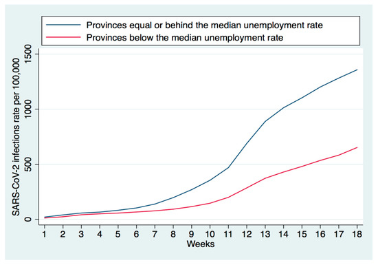
Figure 1.
Infection rates per 100,000 inhabitants per province according to the unemployment rate at the beginning of the pandemic. The period covers the 18 weeks corresponding to 3 April through 31 July 2020. Source: authors’ elaboration based on the Chilean National Employment Survey (ENE) and “Open COVID-19 Data” provided by the Ministerio de Ciencia Tecnología, Conocimiento e Innovación de Chile (Chilean Ministry of Science and Innovation).
We estimated two curves according to the position over or under the median unemployment rate at the beginning of the pandemic. To calculate the unemployment rate prior to the pandemic, the three mobile quarters between November 2019–January 2020 and January–March 2020 provided by the ENE were considered. The median unemployment rate was 6.97%.
3. Empirical Analysis
To empirically test the defined hypothesis, we propose to use the following equation for estimation:
The variable corresponds to the SARS-CoV-2 infection rate per 100,000 inhabitants on the last available date of the analysis, 31 July 2020, for each province analyzed. This information was obtained from the “Open COVID-19 Data” provided by the Ministerio de Ciencia Tecnología, Conocimiento e Innovación de Chile (MCTCI) (Chilean Ministry of Science and Innovation), which records the accumulated cases that have been confirmed as positive for SARS-CoV-2 at municipal level. We aggregated municipal information in provinces due to the lack of statistical representativeness of small-size municipalities.
The variable represents the variable of interest in the analysis and reflects the situation of the labor market in each province at the beginning of the pandemic in Chile via the following variables:
- employment rate in each province ();
- unemployment rate in each province ();
- extended unemployment rate, which includes the population outside the labor force who could be potential participants in the labor market ().
The extended unemployment rate measures the number of people seeking employment and/or those that could have done so prior to the pandemic, but who may have seen their search process limited due to the Social Outbreak. This data comes from the National Employment Survey for the three mobile quarters immediately before the pandemic: between November 2019–January 2020 and January–March 2020. These dates were chosen as they reflect the consequences of the Social Outbreak with regard to the labor market. It is important to highlight that the ENE sampling carried out at the provincial level might not have been representative for smaller provinces; therefore, we increased the sample size by considering the three quarters together, which reduced the measurement error in the indicators used. In this sense, 52 of the 56 provinces in Chile were available in the study.
The variable represents the K control variables used in the model that could have had an impact on the spread of the disease in each province. These variables collect determinants of the pandemic that have previously been considered in other studies: (i) the population density in each province in 2019 (inhabitants/km2) () according to the annual estimate conducted by the National Institute of Statistics (INE); (ii) the number of people living in a situation of critical overcrowding over the total population by province (), calculated in 2017 by the Urban Observatory of the Chilean Ministry of Housing and Urbanism; (iii) the population aged 65 and above over the total population, according to the last census carried out (year 2017) (), with data provided by the INE [20]; (iv) the number of people employed in mining per province over the total population at the beginning of the pandemic () (data provided by the INE). This variable was included because mining activity has not ceased operations during the pandemic and has become a potential source of disease transmission through the continuous flows of workers resulting from the fly-in fly-out (FIFO) system of work predominant in this industry [21]. Finally, identifies dummies by region in order to control the heterogeneity not observed at this territorial level.
Additionally, given that the estimate was sensitive to the way the spatial units of analysis were defined, new estimates of Equation (1) were made by grouping the provinces according to the labor market functional areas (LMFAs) defined by [22], resulting in 135 different LMFAs for Chile. This methodology is relevant to the analysis since the administrative limits defined in the territories (provinces) are not sufficient to provide a perfect delimitation for a single labor market, as in many cases this area could extend beyond those administrative borders [23]. This new delimitation of the spatial units allows a correct interpretation of the area through which the workers move, and therefore potentially the disease. Furthermore, as a robustness analysis, Equation (1) can be estimated with all the periods available in the sample, which were the 18 weeks from 3 April to 31 July, a period which corresponds to the first wave of the disease in the country. For this, a random effects panel data methodology was used with an autoregressive of order 1 (AR (1)) structure in the residuals in order to correct the potential serial correlation in the model derived from the dynamic feedback that could exist in the number of infected [24].
4. Results
Table 2 shows the results obtained when estimating Equation (1), using the provinces as the unit of analysis for both the last period (columns 1 to 6) and for the 18 weeks available between 3 April to 31 July (columns 7 to 9). These results reject a priori the thesis that the labor market variables from prior to the pandemic impacted the number of accumulated infections per 100,000 inhabitants (for the latest available date). We observe a similar result for the number employed in mining over the total population. However, when all available periods are considered, the results show a positive and significant impact for the higher rate of critical overcrowding and the population density on the number of infected. A negative relationship can be observed for the infection rate of people over 65 in the population.
Table 2.
Estimates of Equation (1) using the sample of provinces.
However, when using the LMFA to estimate Equation (1), the results change substantially with respect to those previously obtained for the provinces, with significant evidence for the relationship established in our hypothesis. When territories that constitute a single labor market are grouped together, we were able to generate a more precise approximation of the flow of people moving through a given space (instead of considering the administrative limits of each province). The variables related to the initial conditions in the labor market are significant in explaining the level of infection rate per 100,000 inhabitants (Table 3). Specifically, these results can be observed for unemployment rates, both conventional and extended, in all the estimates made. The number of people infected by SARS-CoV-2 in each LMFA increases by approximately 50–70 people per 100,000 for each additional percentage point in the unemployment rate prior to the pandemic for the last period analyzed (columns 2, 3, 5 and 6); when all the available weeks are considered (columns 8 and 9), the estimated coefficient for unemployment is close to a value of 15.
Table 3.
Estimates of Equation (1) grouping the municipalities in labor market functional areas.
This result is relevant as it provides evidence for the relationship between unemployment prior to the pandemic, a situation that deteriorates the income capacity of households and reduces the effectiveness of confinement policies [12], and the spread of the disease. Furthermore, these results, like the models based on provinces, show that population density and critical overcrowding have a positive and significant impact on the number of infections, while the infection rate of the population over 65 years old shows a significant but negative effect. A potential explanation for the negative and significant coefficient estimated for the population over 65 years old is that this group is not typically part of the labor market and so mobility is not required. Additionally, this segment of the population is more vulnerable to SARS-CoV-2 and therefore more willing to abide by confinements than other age groups. The rest of the variables considered in the analysis (the employment rate prior to the pandemic and employment in mining) were not statistically significant in explaining the number of infected per 100,000 inhabitants in any of the estimates made. This last variable probably deserves a more specific analysis focused on the case of mining regions that receive flows of workers from other regions.
In order to deepen the analysis, we made new estimates via pooled ordinary least squares (pooled OLS) that show how the equilibrium of the labor market prior to the pandemic was able to impact not only the number of people infected by SARS-CoV-2 (accumulated at the latest available date), but also the dynamics of the epidemic at the national level. To do this, we considered all the weeks available in the study. The new equation to estimate is as follows:
The variable considers the number of SARS-CoV-2 infections per 100,000 inhabitants in each of the territories, whether provinces or LMFAs, and the weeks available (). The variable represents a time-fixed effect for each of the 18 weeks considered. Our interest was focused on the estimation of , a coefficient that is associated with the interaction between and the variables that define the situation of the labor market in each territory at the beginning of the pandemic.
The results of the interaction are represented in Figure 2. They once again show that the unemployment rate (in its two dimensions) had a positive and significant impact on the number of SARS-CoV-2 infections per 100,000 inhabitants starting in the weeks 10–11 (corresponding to the first two weeks of June) and continuing throughout the period analyzed, both for the analyses carried out by provinces and LMFAs. Before this date, no significant impact from unemployment on the pandemic was observed except for in the LMFAs, where the estimated coefficients were slightly negative and significant. For the last date (week 18), the coefficients associated with the interaction in the analysis applied to the provinces were between 130–150 infected per 100,000 inhabitants and for the LMFAs somewhat lower (approximately 50). This may have been related to the fact that the LMFAs have a lower population on average than the provinces. The interaction applied to the employment rate was not significant, a similar result to that previously observed.
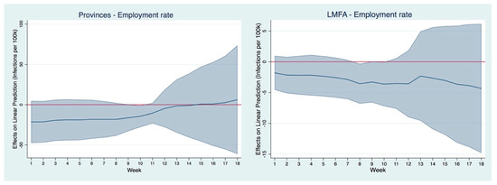
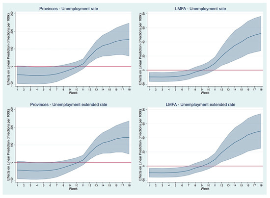
Figure 2.
Estimates for the interactions between the variables that defined the equilibrium of the labor market at the beginning of the pandemic and the time effects for the 18th week of its duration until 31 July 2020, in Chile. (i) The blue line represents the coefficients estimated. (ii) The light blue area represents confidence intervals. (iii) The red line represents zero value.
The estimates reflect differentiated behavior between the territories (whether they were provinces or LMFAs) during the second week of June and thereafter, dependent on the level of unemployment at the beginning of the pandemic. This may have been related to the fact that the first imported cases of SARS-CoV-2 were strongly concentrated in the municipalities with the highest income and therefore the greatest resources to face the pandemic. The disease soon spread to the rest of Chile and the areas with the worst labor market equilibrium prior to the pandemic (due to the impact of the Social Outbreak and the subsequent economic deterioration) were those that experienced a more significant loss in their earning capacities [25,26,27]. This could also have been related to a lower capacity to comply with the confinement policies due to an inability to meet consumption needs by strictly staying at home [12].
With the evidence obtained so far, it is reasonable to think that the Social Outbreak had a direct impact on the worsening of labor market indicators (particularly in terms of unemployment) prior to the arrival of SARS-CoV-2 in the country [17], which subsequently impacted the dynamics of the infection rate per 100,000 inhabitants from the first half of June.
A potential hypothesis explaining these results is that, as the pandemic progresses, areas that were in a worse situation in terms of the labor market prior to the pandemic may have experienced greater labor mobility. This could also have been related to a lower capacity to comply with containment policies and a higher rate of infections per 100,000 inhabitants. For many, staying at home means not meeting their consumption needs [12].
The effect that the pandemic may have had on areas with higher levels of unemployment prior to the pandemic could have been an increase in labor market activity in order to offset the potential decrease in household income. To test this new hypothesis, we followed the theoretical framework proposed by the job-search model [28], according to which the probability of actively participating in the labor market (, otherwise) positively depends on the probability that an individual has of accepting a job offer, which is conditioned to their reservation wage (), as follows:
where represents the monetary value of non-labor income, is the cost of the search that positively depends on the effort applied ( and the SARS-CoV-2 infection level (). If infections are high, the risk of contracting the disease increases, which increases the cost of the job search . The variable is the probability of receiving a job offer which depends on the search effort , represents the temporary discount factor, is the expected wage of the offer received and is the cumulative distribution function of the wage offered.
Following this framework, we estimated the following model of simultaneous equations:
The variable defines the rate of labor activity during the pandemic (considering the average for the aggregation of data corresponding to mobile quarters February–April, March–May, April–June and May–July 2020 for the ENE) for each of the territories, either provinces or LMFAs. refers to the rate of SARS-CoV-2 infected per 100,000 inhabitants as of 31 July 2020. Regarding Equation (5), the same regressors used to estimate Equation (1) were used.
The estimation method used for the structural simultaneous equations system defined by Equations (4) and (5) was Three-Stage Least Squares (3SLS) since it allowed us to exploit the correlation of the disturbances across equations and improved the efficiency of the estimates. This was under the assumption that there might have been different unobserved elements that jointly affected and . The results obtained are presented in Table 4 and show a positive relationship between the SARS-CoV-2 infection rate per 100,000 inhabitants and the activity rate during the pandemic period in all the estimates made (estimates for Equation (4)), both for the provinces and for the LMFAs. However, with regard to the product of the estimated parameters (), which indicates the effect that those variables related to the labor market prior to the pandemic have had on work activity during the pandemic, the results were positive for all estimates, but mostly not significant for all of them. Therefore, there is no evidence that the labor market situation at the beginning of the pandemic positively impacted labor activity or mobility.
Table 4.
Three-Stage Least Squares (3SLS) estimates of Equations (4) and (5) using the samples of both provinces and labor market functional areas (LMFAs) in June (last month available for labor market statistics).
On the other hand, it is important to bear in mind that the Chilean economy had already experienced a deterioration in its economic growth and the labor market before the Social Outbreak, primarily due to the end of the mining prices super cycle since 2011. In fact, [16] (p. 10) states that “since 2014, Chilean GDP growth has remained below 3.0%, which has generated less dynamism in job creation”. Unemployment in Chile increased steadily between 2015 and 2019, growing by 24.7%. This rise was primarily due to an increase in the workforce during that period, in which approximately 815,800 people joined the labor supply, but the employment rate remained at 58% (between 2015 and 2019 there were about 677,600 jobs created). However, working conditions deteriorated substantially, with self-employment and informal employment growing significantly, both of which present lower income levels and are of lower quality than salaried employment [16].
Therefore, taking into consideration the outcomes obtained in Table 2 and Table 3 and Figure 2, it is worth asking if the deterioration seen in the labor market because of the Social Outbreak was only a reflection of the inertia of the end of the super cycle and the subsequent deterioration in economic dynamics, and whether this previous worsening, via growth in unemployment, impacted the number of SARS-CoV-2 infections at the national level. To test this hypothesis, the estimates of Equation (1) presented in Table 2 and Table 3 were repeated. In this case, the variable (which represents the labor market situation in each territory in Chile at the beginning of the pandemic using the unemployment, extended unemployment and employment rates) was calculated using all the available mobile quarters from the ENE for each year within the period 2011–2019. In this way, the 12 quarters from December–February (first of the year) to November–January (last) were considered for each year of that period.
The estimated coefficients for are presented in Table 5 and Table 6. Despite some significant results, the coefficients do not show a clear significant trend that was repeated in subsequent years. For example, the significant effect obtained for 2016 was not obtained for 2017, 2018 or 2019, something that could be explained by a spurious correlation rather than the end of the mineral super cycle, which presented a persistent impact on growth and employment between 2015 and 2019 [16]. All of this reinforces the idea that the effects of the Social Outbreak on the deterioration in the job market and the increase in unemployment (and the subsequent loss of income) are factors in understanding the high rate of infections in Chile during the pandemic. In contrast, there is no strong evidence that this result was due to the inertia of the end of the commodity super cycle and the subsequent worsening of economic conditions.
Table 5.
Estimates of Equation (1) using the sample of provinces.
Table 6.
Ordinary least squares estimates of Equation (1) grouping the municipalities in labor market functional areas (Berdegué et al. 2017).
5. Conclusions
This study evaluated how the influence of economic conditions, and the particularly labor market, impacts the control of the pandemic. The results show that the unemployment rate at the beginning of the disease is a key variable for understanding its progression, as seen in one of the developing countries most affected by it during the first half of 2020. In the case of Chile, one explanation can be found in the social disturbance that occurred in the latter part of 2019 and which negatively impacted economic growth and significantly raised the level of unemployment [17].
On the other hand, we observe that the effect of unemployment at the beginning of the pandemic was not immediate but rather started in the second week of June. It took approximately three months for the divergence between the territories with the highest unemployment rates prior to the pandemic and those that started with a better situation. This result may have been due, in part, to the fact that the first imported cases occurred in the higher-income areas of the country and may also be related to the progressive deterioration of the income of families affected by unemployment at the beginning of the pandemic, something that it has worsened, limiting growth and deepening the destruction of jobs. In this sense, some studies have indicated that lower-income households (those more likely to have lower-quality jobs and/or be unemployed) are the ones with the greatest mobility throughout the pandemic, having to participate in work activity outside their homes to maintain their income level [18,19]. However, our results do not show that the situation in the labor market at the beginning of the pandemic, whether unemployment (with its two different measures) or employment, increased labor activity in the last period observed. Therefore, a priori, it can be ruled out that this would have had an impact on the increase in mobility and, subsequently, infection rates. However, it is likely that the official data on work activity is underestimated, as there are incentives on the part of individuals receiving pandemic aid to not declare their work activity/income due to the risk of losing these benefits [18]. Therefore, these results could be biased. Primary information is needed to validate the relationship found.
However, an additional factor that may also have influenced the mobility of the unemployed is that they have had to carry out a large number of activities, many of them related to obtaining social benefits, such as unemployment insurance and other grants or help offered by the government [25], for which, in many cases, it is preferred (or required) to be present in person. At the onset of the pandemic, Chilean media reported “long lines” in municipal offices relating to concerns about how to request government food boxes or update the social registry of households, a necessary procedure for obtaining social benefits.
The aforementioned elements resulting in the greater mobility of the unemployed and more vulnerable households are only hypotheses, as they have not been addressed in the present study due to the lack of reliable data. For this reason, it is essential to expand the collection of information on mobility within territories, not only for Chile but also for any country that began the pandemic with a disadvantageous economic context. It is also important to highlight that the present study has limitations derived from the aggregation of the data. Mobility decisions are influenced by participation in work activity, something that is decided at the intra-family level [29]. These data do not currently exist but would provide greater detail on how households were organized to face the pandemic.
This study aims to better understand the channels through which the previous economic conditions were able to influence the spread of the pandemic and to identify and define appropriate policies for controlling its spread in the present and immediate future. At the end of this research, we still have no certainty regarding an end to the pandemic but it seems likely that any recovery in the short term will be relatively slow and that the risk of a second or even third wave is high, not only in Chile but also in other Latin American countries. This entails the need for further research to improve the comprehension of the effects of initial social and economic conditions in each country and thereby contribute to improving the design of policies aimed at minimizing the health and socioeconomic effects of the pandemic (Table A2 in Appendix A).
Author Contributions
Conceptualization, M.P.T. and M.A.; methodology, M.P.T. and M.A.; software, M.P.T.; validation, M.P.T. and M.A.; formal analysis, M.P.T. and M.A.; investigation, M.P.T. and M.A.; resources, M.P.T. and M.A.; data curation, M.P.T.; writing—original draft preparation, M.P.T. and M.A.; writing—review and editing, M.P.T. and M.A.; visualization, M.P.T. and M.A.; Both authors have read and agreed to the published version of the manuscript.
Funding
This research received no external funding.
Institutional Review Board Statement
Not applicable.
Informed Consent Statement
Not applicable.
Data Availability Statement
The data presented in this study are available on request from the corresponding author.
Conflicts of Interest
The authors declare no conflict of interest.
Appendix A
Table A1.
ANOVA for the rate of infections per 100,000 inhabitants by continent on 31 July 2020 (last date available for the analysis).
Table A1.
ANOVA for the rate of infections per 100,000 inhabitants by continent on 31 July 2020 (last date available for the analysis).
| SARS-CoV-2 | Mean of SARS-CoV-2 Infection Rate per 100,000 Inhabitants ^ | |
|---|---|---|
| Africa | 5530.67 (4657.2) | |
| Asia | 12,668.32 (6884.44) | |
| Europe | 37,142.40 (8243.81) | *** |
| North America | 43,262.96 (10,992.80) | *** |
| Oceania | 6776.50 (26,753.58) | |
| South America | 81,999.86 (10,413.82) | *** |
| F-test (p-value) | 0.000 | |
Source: author’s elaboration. Standard deviations in brackets. *: Significant at 0.1, **: 0.05, ***: 0.01. ^ Coefficients obtained by applying OLS estimates.
Table A2.
Socio-economic descriptive statistics and infections rate per 100,000 inhabitants * for Latin-American countries.
Table A2.
Socio-economic descriptive statistics and infections rate per 100,000 inhabitants * for Latin-American countries.
| Countries | Emp. Rate (ILO) 2019 (*) INE–ENE Quarter January–March | Unemp. Rate (ILO) 2019 (*) INE–ENE Quarter January–March | GDP pc 2019 | GINI Index 2018 (*) 2017 Last Data Available | Poverty Headcount Ratios at National Poverty Lines (% of Population) 2018 (*) 2017 Last Data available | Infections Rate per 100,000 31 July 2020 |
|---|---|---|---|---|---|---|
| Chile | 57.3 (*) | 8.2 (*) | 15,091.5 | 44.4 (*) | 3.6 (*) | 18,605.5 |
| Panama | 64.0 | 3.9 | 11,910.2 | 49.2 | 15,123.9 | |
| Brazil | 56.2 | 12.1 | 11,121.7 | 53.9 | 12,525.8 | |
| Peru | 75.1 | 3.3 | 6486.6 | 42.8 | 20.5 | 12,358.8 |
| Bolivia | 69.3 | 3.5 | 2579.9 | 42.2 | 34.6 | 6578.3 |
| Dominican Rep. | 60.6 | 5.8 | 8002.4 | 43.7 | 22.8 | 6420.5 |
| Colombia | 62.1 | 9.7 | 7838.2 | 50.4 | 27.0 | 5807.6 |
| Ecuador | 65.3 | 4.0 | 5097.1 | 45.4 | 23.2 | 4837.9 |
| Honduras | 65.1 | 5.4 | 2241.2 | 52.1 | 48.3 | 4241.9 |
| Argentina | 55.3 | 9.8 | 9742.5 | 41.4 | 32.0 | 4232.7 |
| Costa Rica | 54.7 | 11.9 | 10,046.9 | 48.0 | 21.1 | 3498.2 |
| Mexico | 58.6 | 3.4 | 10,267.5 | 45.4 | 41.9 | 3293.5 |
| Suriname | 47.4 | 7.3 | 8046.9 | 2812.7 | ||
| Guatemala | 60.8 | 2.5 | 3413.2 | 2779.1 | ||
| El Salvador | 56.7 | 4.1 | 3572.4 | 38.6 | 26.3 | 2564.2 |
| Paraguay | 68.6 | 4.8 | 5310.4 | 46.2 | 24.2 | 748.4 |
| Venezuela | 54.5 | 8.8 | 653.2 | |||
| Haiti | 57.9 | 13.8 | 1245.0 | 651.1 | ||
| Nicaragua | 61.9 | 6.8 | 1763.2 | 554.3 | ||
| Guyana | 49.5 | 11.9 | 6107.3 | 525.1 | ||
| Uruguay | 58.4 | 8.7 | 14,597.3 | 39.7 | 8.1 | 363.9 |
| Cuba | 52.7 | 1.6 | 6816.9 | 230.3 | ||
| Trin. and Tobago | 58.3 | 2.7 | 15,105.1 | 120.8 |
Source: authors’ elaboration using World Development Indicators and data from Our World in Data (University of Oxford). * Data of infections rate per 100,000 inhabitants were collected for 31 July 2020, last date available for the analysis.

Figure A1.
Daily dynamic of the SARS-CoV-2 total and newly infected by from 4 March until 31 July 2020. Authors’ elaboration based on data from Our World in Data (University of Oxford). A total of 36,179 newly infected cases were added on 17 June 2020, not previously considered in the official figures provided by the Health Ministry.

References
- CEPAL. El Desafío Social en Tiempos del COVID-19; Special Report #3 COVID-19; United Nations: New York, NY, USA, 2020; Available online: https://repositorio.cepal.org/bitstream/handle/11362/45527/5/S2000325_es.pdf (accessed on 4 January 2021).
- Banco Central de Chile. Informe de Política Monetaria, Junio 2020; Banco Central de Chile: Santiago, Chile, 2020.
- Zandi, G.; Shahzad, I.; Farrukh, M.; Kot, S. Supporting Role of Society and Firms to COVID-19 Management among Medical Practitioners. Int. J. Environ. Res. Public Health 2020, 17, 7961. [Google Scholar] [CrossRef] [PubMed]
- International Monetary Fund (IMF). World Economic Outlook, June 2020: A Crisis Like No Other, An Uncertain Recovery; IMF: Washington, DC, USA, 2020. [Google Scholar]
- World Bank. Global Economic Prospects; World Bank: Washington, DC, USA, 2020. [Google Scholar]
- Gerszon, D.; Lakner, C.; Castaneda, A.; Wu, H. The Impact of COVID-19 (Coronavirus) on Global Poverty: Why Sub-Saharan Africa Might Be the Region Hardest Hit; World Bank Data Blogs: Washington, DC, USA, 2020; Available online: https://blogs.worldbank.org/opendata/impact-covid-19-coronavirus-global-poverty-why-sub-saharan-africa-might-be-region-hardest (accessed on 4 January 2021).
- Hall, R.; Jones, C.I.; Klenow, P.J. Trading Off Consumption and COVID-19 Deaths; NBER Working Paper No. 27340; National Bureau of Economic Research: Cambridge, MA, USA, 2020. [Google Scholar]
- Piguillem, F.; Shin, L. Optimal Covid-19 Quarantine and Testing Policies. CEPR Discussion Paper No. DP14613. 2020. Available online: https://ssrn.com/abstract=3594243 (accessed on 4 January 2021).
- Alvarez, F.; Argente, D.; Lippi, F. A Simple Planning Problem for COVID-19 Lockdown; NBER Working Paper No. 26981; National Bureau of Economic Research: Cambridge, MA, USA, 2020. [Google Scholar]
- Barro, R.; Ursúa, J.; Weng, J. The Coronavirus and the Great Influenza Pandemic: Lessons from the “Spanish Flu” for the Coronavirus’s Potential Effects on Mortality and Economic Activity; NBER Working Paper No. 26866; National Bureau of Economic Research: Cambridge, MA, USA, 2020. [Google Scholar]
- Gray, G.; Ortiz-Juarez, E. Temporary Basic Income: Protecting Poor and Vulnerable People in Developing Countries; United Nations Development Programme: New York, NY, USA, 2020. [Google Scholar]
- Das, J.; Sánchez-Páramo, C. Smart Containment: How Low-Income Countries Can Tailor Their COVID-19 Response; World Bank Data Blogs: Washington, DC, USA, 2020; Available online: https://blogs.worldbank.org/voices/smart-containment-how-low-income-countries-can-tailor-their-covid-19-response (accessed on 4 January 2021).
- Molla, A.; Licker, P. eCommerce adoption in developing countries: A model and instrument. Inf. Manag. 2005, 42, 877–899. [Google Scholar] [CrossRef]
- Álvarez, R.; García-Marín, A.; Ilabaca, S. Commodity price shocks and poverty reduction in Chile. Res. Pol. 2018. [Google Scholar] [CrossRef]
- PNUD. Desiguales. Orígenes, Cambios y Desafíos de la Brecha Social en Chile; PNUD: New York, NY, USA, 2017; Available online: http://www.fundacionmicrofinanzasbbva.org/revistaprogreso/en/unequal-origins-changes-and-challenges-in-chiles-social-divide/ (accessed on 18 January 2021).
- International Labor Office (ILO). El Mercado Laboral en Chile: Una Mirada de Mediano Plazo; ILO Informes Técnicos/4 año 2017; ILO: Santiago, Chile, 2018. [Google Scholar]
- Banco Central de Chile. Informe de Política Monetaria, Marzo 2020; Banco Central de Chile: Santiago, Chile, 2020.
- IPSOS & Espacio Público. ¿Cómo se Vive la Cuarentena en la Región Metropolitana? Encuesta IPSOS & Espacio Público. 2020. Available online: https://www.espaciopublico.cl/wp-content/uploads/2020/06/Informe-estudio-de-Movilidad-en-Cuarentena-DISEÑO-OK-FINAL2.pdf (accessed on 4 January 2021).
- MOVID-19. ¿Cuál Ha Sido la Respuesta de la Población a las Cuarentenas? El Impacto de las Desigualdades en la Efectividad de las Politicas Sanitarias. Monitoreo Nacional de Síntomas y Prácticas COVID-19 en Chile. 2020. Available online: https://www.uchile.cl/noticias/164174/efecto-de-la-cuarentena-se-redujo-en-78-luego-de-plan-retorno-seguro (accessed on 4 January 2021).
- Di Porto, E.; Naticchioni, P.; Scrutinio, V. Partial Lockdown and the Spread of COVID-19: Lessons from the Italian Case; Discussion Paper Series IZA #13375; IZA—Institute of Labor Economics: Bonn, Germany, 2020. [Google Scholar]
- Aroca, P.; Atienza, M. Economic implications of long distance commuting in the Chilean mining industry. Res. Pol. 2011, 36, 196–203. [Google Scholar] [CrossRef]
- Berdegué, J.; Hiller, T.; Ramírez, J.; Satizábal, S.; Soloaga, I.; Soto, J.; Uribe, M.; Vargas, O. Delineating functional territories from outer space. Lat. Am. Econ. Rev. 2019, 28, 1–24. [Google Scholar] [CrossRef]
- Casado-Díaz, J. Local Labour Market Areas in Spain: A Case Study. Reg. Stud 2000, 34, 846–856. [Google Scholar] [CrossRef]
- Baltagi, B.; Wu, P.X. Unequaly spaced panel data regression with AR (1) distrubances. Economet. Theor. 1999, 15, 814–823. [Google Scholar] [CrossRef]
- MOVID-19. ¿Cómo Reducir el Riesgo de Contagios de Quienes Trabajan Remuneradamente para Enfrentar la Crisis Social y Sanitaria? Una Mirada desde el Trabajo Remunerado. Monitoreo Nacional de Síntomas y Prácticas COVID-19 en Chile. 2020. Available online: https://www.movid19.cl/informes/mesasocial8.html#2_situación_actual_de_los_mercados_del_trabajo (accessed on 4 January 2021).
- Inchauste, G.; de Hoop, J.; Saavedra, T. Crisis de la COVID-19 Podría Revertir Años de Crecimiento de la Clase Media Chilena; World Bank Data Blogs: New York, NY, USA, 2020; Available online: https://blogs.worldbank.org/es/latinamerica/crisis-de-la-covid-19-podria-revertir-anos-de-crecimiento-de-la-clase-media-chilena (accessed on 18 January 2021).
- Jiménez, A.; Duarte, F.; Rojas, G. Sindemia, la Triple Crisis Social, Sanitaria y Económica; y Su Efecto en la Salud Mental; CIPER/Académico: Santiago, Chile, 2020; Available online: https://www.ciperchile.cl/2020/06/20/sindemia-la-triple-crisis-social-sanitaria-y-economica-y-su-efecto-en-la-salud-mental/ (accessed on 4 January 2021).
- Mortensen, D. Job Search, the Duration of Unemployment, and the Phillips Curve. Am. Econ. Rev. 1970, 60, 847–862. [Google Scholar]
- Chiappori, P.-A. Collective labor supply and welfare. J. Pol. Econ. 1992, 100, 437–467. [Google Scholar] [CrossRef]


Publisher’s Note: MDPI stays neutral with regard to jurisdictional claims in published maps and institutional affiliations. |
© 2021 by the authors. Licensee MDPI, Basel, Switzerland. This article is an open access article distributed under the terms and conditions of the Creative Commons Attribution (CC BY) license (http://creativecommons.org/licenses/by/4.0/).