Retirement Age and Housing Consumption: The Case of South Korea

Abstract

South Korea became an aging society in 2000 and will become a super-aged nation in 2026. The extended life expectancy and earlier retirement make workers’ preparation for retirement more difficult, and that hardship might lead to poorer living conditions after retirement. As annuity payments are, in general, not enough for retirees to maintain their previous standard of living after retirement, retired households would have to liquidate their financial and real assets to cover household expenditures. As housing takes the biggest share of households’ total assets in Korea, it seems to be natural for retirees to downsize their houses. However, there is no consensus in the housing literature on housing downsizing, and the debate is still ongoing. In order to understand whether or not housing downsizing by retirees occurs in Korea, this paper examines the impact of the timing of retirement on housing consumption using an econometric model of housing tenure choice and the consumption for housing. The results show that the early retirement group living in more populated region does not downsize the house, while the timing of retirement is negatively associated with housing consumption for the late retirement group living in the peripheral region.

1. Introduction

Aging is a global issue. According to the definition of the United Nations, when people aged 65 or older account for 7–14 percent of the population, it is called an aging society; when the proportion is between 14 and 20 percent, it is called an aged society; when it is over 20 percent, it is called a super-aged society. For example, Japan, where aging has been taking place more rapidly, became an aging society in 1970, entered an aged society in 1994, and has been a super-aged society since 2005 [1]. South Korea (hereafter, “Korea”) is also one of the most rapidly aging countries, with a decreasing birth rate. Korea became an aging society in 2000 and an aged society in August 2017, and will become a super-aged country in 2026.

In 2015, the residual expected life at 65 in Korea was 18.2 years for men and 22.4 years for women. Those numbers have increased over the past 10 years [2]. On the contrary, workers tend to retire earlier prior to the age of 60, even though 60 marks formal retirement. This extended life expectancy and earlier retirement make workers’ preparation for retirement more difficult, and that hardship might lead to poorer living conditions after retirement [3,4]. In Korea, only 6.7 percent of retired households have “enough” provisions for living expenses, while 42.2 and 20.9 percent have “insufficient” and “very insufficient” provisions, respectively [5]. In addition, the relative poverty rate for households with household heads aged 66 or older is 53.1 percent. These figures reveal that a significant portion of retired households encounter financial difficulties after retirement. Most retired people rely on annuity income instead of earned income, but annuity payments are generally not high enough to prepare for a satisfactory standard of living after retirement [6,7,8]. In Korea, 45.3 percent of people aged 55 to 79 received an annuity of KRW (South Korean won) 520,000 (about USD 444 as of 20 September 2020) per month in 2016, and 73 percent received less than 500,000 won [9]. This means that most elderly face difficulties in living a financially stable life. Owing to this insufficient annuity, some retirees who own multi-unit properties let a portion of their residential properties to earn rental incomes [10,11,12].

There are many people who do not save enough money in preparation for retirement, and they are thus not likely to have the essential financial resources required to maintain their standard of living in retirement [13]. This reality seems to be more significant for the early retirement group. Fisher et al. [14] expected that people who retire early are more likely to spend their wealth compared to individuals who work longer. Retiring early might mean that people have to rely upon their previously accumulated wealth for a longer amount of time.

As houses are the largest assets owned by most households, do retirees downsize their houses? Among these retirees, who downsizes their houses? There is no consensus in the housing literature on housing downsizing, and the debate is still ongoing. On the one hand, retired households downsize their homes for the consumption of non-durable goods after retirement. Those households plan properly for retirement, which supports the life-cycle income hypothesis and the notion of consumption smoothing. According to this premise, in retirement, accumulated assets are decumulated to achieve the desired level of consumption of non-durable goods and services. On the other hand, there is an opposing strand of literature which found a sharp decline in consumption during the early years of retirement. One reason for this “retirement-consumption” puzzle might be the unwillingness or failure to downsize financial and real assets.

This study contributes to the existing literature on the demand for housing by comprehensively considering the simultaneous linkage of housing tenure choice and housing consumption using a rigorous statistical treatment. Specifically, we first calculated the likelihood of owning a house using a logit model. Then, the estimated propensity of home ownership was included in the housing consumption regression equation as an explanatory variable, in order to deal with the simultaneity between housing tenure choice (owning versus renting) and the consumption for housing (dwelling size). We used the 2014 Survey of Household Finances and Living Conditions (SFLC) dataset provided by Statistics Korea. The dataset contains socio-demographic and financial information for households of all generations. We extracted a sample of retired households from the data. Our analysis was divided into four sub-categories by retirement group and region. We posit that retirees show different housing consumption patterns with respect to the timing of retirement. We estimated the housing downsizing equations for the capital region (Seoul, Gyunggi, and Incheon) and for the non-capital region separately, due to the spatial heterogeneity of the housing market in Korea.

This paper is organized as follows. Section 2 discusses the previous literature on retirement and housing. Section 3 describes the data, variables, and research methodology. Section 4 presents the results from housing tenure choice and housing consumption regressions by retirement group and region. In Section 5, we discuss the results of housing downsizing and their implications for the formation of housing policies for older or retired households. Finally, Section 6 provides some brief concluding remarks and the limitations of the research.

2. Related Literature

2.1. Definition of Retirement

Studies on retirement have employed different definitions of retirement. It can be defined by whether one participates in an economic activity. If one provides a positive answer to the question “Have you completely stopped working or looking for a job?”, one is considered to be a retiree [15]. Another definition is related to a significant change in working hours or wages. When one’s working hours or wages drastically drop below a certain threshold, one is considered to be a retiree [16,17]. This can also be defined by whether one has left one’s primary workplace. If a worker has left the workplace in which he or she has worked for the longest period of time, the person is considered to be a retiree, regardless of current job activities [18,19,20,21]. Whether or not one receives a retirement annuity can also define the status of retirement. When one receives a public or private annuity, one is a retiree [22]. Finally, retirement is defined by one’s subjective assessment. If one provides a positive answer to the question “Are you currently retired?”, one is considered to be a retiree [23,24].

The SFLC data used in this study contain the respondents’ subjective assessment. Additionally, retirement is formally defined in South Korea as “the state of being retired from one’s business or occupation.” First, this study defines retirees as those who answered “yes” to the question “Are you currently retired?” in the SFLC. As for the age cut-off, we also included the early retirement group. Korea’s effective age of retirement is around 68 for men and 67 for women. These figures are much higher in many other OCED (Organization for Economic Co-operation and Development) nations. Firms, however, tend to be reluctant to employ older workers. Accordingly, many employers in Korea often set the “mandatory retirement” policy, by which they lay off older workers below the age of 60, as low as 55 [25]. In the SFLC, we observed that some retirees listed their retirement ages as being below 60. We chose to include retirees whose retirement age was equal to or greater than 50, following the study by Kim and Son [26]. The formal retirement age in Korea is 60, similar to many countries. Therefore, we define retirees whose retirement age ranges from 50 to 59 as the “early retirement group”, and retirees from the age of 60 to 80 as the “late retirement group”. We excluded retirement ages of 81 or above from the analysis.

2.2. Literature on Housing and Retirement Timing

There are a handful of studies in retirement literature that explore the role of housing in retirement timing. Szinovacz et al. [27] studied the effects of wealth and investment on retirement timing, and found that a decrease in home value is positively related to expectations to work after the age of 62, although the effect is modest relative to other determinants, such as debts and the work environment [28,29]. Farnham and Sevak [30] investigated the effect of the change in housing wealth using the Health and Retirement Study (HRS). They found that a 10 percent increase in housing wealth is associated with a decrease in the expected retirement age of between 3.5 and 5 months. Hartig and Fransson [31] assessed the association between housing tenure and early retirement, and found that housing circumstances have an impact on retirement timing. On the other hand, Gorodnichenko et al. [32] found that home values in the United States have nothing to do with retirement timing, while unemployment rate and inflation are important factors. Similarly, Disney et al. [33] found little evidence of any wealth (housing prices or share prices) effects on retirement timing from the British Household Panel Survey.

2.3. Literature on the Consumption for Housing of Retirees

Home ownership is a major way to accumulate assets for later life in Korea. Some elderly people might earn rental incomes by holding assets other than houses. Kim and Jeon [34] found that this phenomenon is observed above a certain income decile in South Korea. They showed that the probability of owning additional houses for lease income increases when the household head is married and has school-age children. Similarly, Lin et al. [35] suggested that those who have a higher price-to-income ratio can buy housing for investment purposes in Taiwan. Disney et al. [36] found that there is a strong connection between asset evolution and retirement behavior for later cohorts of retirees in Britain.

The biggest portion of the portfolio of retirees comprises housing assets compared to financial assets in many countries [37]. In Latin America, 90 percent of householders aged 64 or older live in their own houses, whereas only 4 percent live in rented housing [38]. In Taiwan, the older the household head is, the more he or she prefers to buy housing [39]. People aged 60 or older in Hong Kong desire to live in their own housing [40]. This preference for housing assets results from the tendency of the middle-aged and elderly to hedge the risk associated with rent changes in the future by possessing their own housing [41]. In addition, those middle- to old-aged people with real estate assets are more financially well off and better prepared for retirement than those without such assets [10,12]. In Japan, the number of aged people who have their own housing is rising because of the government policy to increase housing welfare by promoting the possession of housing in the postwar period [42].

On the other hand, some studies show that retirees switch from owning to renting or downsize their homes, which is in accordance with the life-cycle income hypothesis [43,44,45,46]. Chiuri and Jappelli [47] found that home ownership declines after the age of 70 in most countries by using an international cross-sectional dataset. Older Americans adjust their housing size by around 0.7 of a room smaller than their previous residence [48]. Yogo [49] found that the housing portfolio is negatively related to health for retirees and falls significantly as they age. On the contrary, other studies suggest that such downsizing or reduction is not closely related to aging and retirement [17,50,51,52,53,54,55].

According to the traditional life-cycle model, retired households who want to reduce the consumption of housing services can liquidate their housing assets through housing downsizing. Artle and Varaiya [56] extended the life-cycle hypothesis to housing, assuming that older households would consume their share of housing after retirement, and predicted that homeowners would convert to rent after retirement. In addition, in the study by Jones [57], the possibility of shifting owning to renting displays a negative relationship with the amount of savings, which is interpreted to support the life-cycle hypothesis. Furthermore, he proposed a revised life-cycle hypothesis, which addresses the fact that housing assets can be liquidated after a significant portion of non-housing assets have been consumed.

However, as many older households were observed to behave differently from the prediction of the life-cycle hypothesis, several alternative hypotheses were suggested. For example, it is argued that socio-demographic changes can lead to tenure transition by reducing the preference for home ownership [52]. They found that the more liquid assets elderly households retain, the lower the probability of housing size reduction becomes.

Venti and Wise [58] conducted a regression analysis of the relationship between the characteristics of moving to owning and the value of housing assets. They found that households with a low income and high housing assets reduce housing assets, while those with a high income and low housing assets increase housing assets. This study revised the life-cycle hypothesis, arguing that homeowners are not moving in order to alleviate liquidity constraints. Some Korean studies, however, found that the liquidity of real estate assets of retirees would be of great importance for their retirement preparation [23,59,60,61].

2.4. Summary

In summary, the concept of retirement is somewhat ambiguous, and the definition of retirement is context-dependent. The status of retirement can be judged by an abrupt change in the working hours or wages, by a change of a person’s prior major workplace, or by whether or not he or she is in receipt of a retirement pension. The retirement literature is not conclusive about the role of housing in the timing of retirement. A decrease in the housing value might accelerate the timing, and that effect would be less significant, relative to other economic conditions, such as unemployment and inflation. Older households might end up with a bigger housing asset or owning a house. In some cases, they eventually downsize their houses. There are, however, other studies that found little evidence on housing downsizing.

3. Research Methodology

3.1. Data and Variables

The SFLC is an annual survey that has been jointly conducted by Statistics Korea, the Financial Supervisory Service, and the Bank of Korea since 2012. The purpose of the SFLC is to support policymaking and research on finance and welfare by comprehensively identifying households’ standards of living and the factors affecting their size composition and distribution of assets, debt, and income [2]. This study used the SFLC 2014 data because the sampling design was altered from a fixed panel to a rotating panel in 2015. For our data, 8907 of the 10,000 households provided a complete response for the “Welfare” section of the survey in SFLC 2014. Among those 8907 households, 1454 stated that “the household head has retired.” After applying our definition of retirement, we obtained 1337 observations as the effective sample for the analysis.

The dataset was further processed in several ways, in accordance with the purpose of the research. The observations, the retirement age of which is less than 50 and greater than 80, were removed. Then, if the household head was not married or divorced, those households were excluded from the study so that only households with the household head being married or widowed were included. This removal was conducted because there are only 13 and 90 cases for unmarried and divorced households in the data, respectively, and the numbers are thus too small to represent those household groups. Furthermore, cases were removed where other household members (except for the household head and his or her partner) were living with the household head. If a retiree is living with other people (such as his or her children or other relatives), the housing consumption for those households should be systematically different, even after controlling for the timing of retirement. As a result of narrowing the scope of household formation, we ended up focusing on households in one of the following two cases: (i) two-person households with one household head with his or her partner, or (ii) one-person households with one widowed household head without any other family member living together with the household head.

The definitions and measurements of the variables used in this study are presented in Table 1. The housing tenure type (HTENURE) is a dummy variable, which takes on the value of 1 if a retired household owns a house. The dwelling size per household member (AREAPM) represents the consumption for housing. Clark and Deurloo [62] used the housing size per household member to examine the housing over-consumption behavior for retired households. The dwelling size variable was logged to be used in the regression equations. The probability of owning a house (OWNPROB) was estimated using demographic and financial variables, and the likelihood variable was then used as an explanatory variable in the housing consumption equation. AGE is the age of the household head in years. AGERE represents the retirement age of the household head, indicating the timing of retirement. We wanted to observe the relationships between the retirement age variable and the consumption for housing by region and retirement group. MSTATUS indicates the marital status of the household head, which takes on a of value of 1 if a retiree is married and lives with his or her partner, and 0 if he or she is widowed and lives alone. Other types of household member formations were not considered in this research. NETINC is the net income variable. We calculated it by subtracting the retired household’s expenditures from the total income. The expenditures include consumption expenditures (groceries, residence, education, healthcare, transportation, communication, and family events) and non-consumption expenditures (tax and social insurance fees). NETASSET is the net asset variable. A retired household’s assets consist of financial and real assets. The financial assets include savings and security deposits. The real assets comprise real estates, automobiles, golf and/or resort membership, jewelry, antiques, and artworks.

Table 1. Definitions of variables.

Variable	Variable Definitions
HTENURE	Housing tenure type (1: Own; 0: Rent)
log(AREAPM)	Logarithm of dwelling size per household member (m2)
OWNPROB	Probability of owning a house
AGE	Age of the household head (years)
AGERE	Retirement age of the household head (years)
MSTATUS	Marital status of the household head (1: Married and living with the partner; 0: Widowed and living alone)
NETINC	Yearly net income of the household
NETASSET	Net asset of the household
CAPITAL	Location of the household (1: National capital region; 0: Remainder of the region)
APT	Housing type of the household (1: Apartment; 0: Other types)

3.2. Empirical Strategy

We recognize that choosing whether to own or rent a house involves an endogenous decision-making process with regard to consumption for housing. King [63] constructed an econometric model of the joint tenure and consumption decision, where both discrete (tenure choice) and continuous (the quantity of housing services) variables are considered using cross-section data. Goodman [64] estimated a joint tenure choice-housing demand model. Ahmad [65] utilized a similar approach for the Karachi housing market. Those studies suggest that ignoring the simultaneity can result in biased elasticity estimates in the equation of housing services. Some studies employed Heckit-type models in regard to the remedy for the simultaneity problem. This study utilized a more direct and intuitively appealing approach, suggested by Fan and Yavas [66], which used the method to study the effect of having a mortgage on household expenditure. In order to tackle the endogeneity problem between housing tenure choice and the level of housing consumption, we first estimated the probability of owning using a logit model. Then, the estimated probability was entered into the housing consumption regression equation as an explanatory variable. The two-step process is as follows:

$$\begin{array}{c}Prob\left(ownin{g}_i=1|X_i\right)={\widehat{owning}}_i=F\left(X_i^T\gamma \right)\\ \log \left(AREAPM\right)={\beta }_0+{\beta }_1{\widehat{owning}}_i+{\beta }_{2}AGERE+{\beta }_3{\mathsf{\Omega }}_i+{\epsilon }_i,\end{array}$$

(1)

where $ownin{g}_i$ indicates whether or not a retired household owns a house and $X_i$ is a vector of independent variables that affect the household’s decision on owning a house. These variables include household demographic and financial characteristics (age of household head, age of retirement, marital status, and net asset), the type of house (apartment or not), and the location of a house (capital area or not). $X_i^T$ is the transpose of the matrix $X_i$, and $\gamma$ is a vector of parameters for $X_i$. $F$ is the cumulative distribution of the logistic distribution. ${\widehat{owning}}_i$ denotes the estimated probability of home ownership. $\log \left(AREAPM\right)$ indicates the natural log of the level of housing consumption, which is measured as the log of the dwelling size of a house per household size—the number of household members. ${\mathsf{\Omega }}_i$ is a vector of explanatory variables that include the same variables as in $X_i$, plus the current net income stream. The two-step procedure enables us to test whether or not the probability of owning is significantly associated with the consumption for housing by checking the significance of ${\beta }_1$. Concerning the robustness for the housing consumption equation, a propensity score matching (PSM) analysis was conducted (see Appendix A).

We chose not to include current income in the housing ownership equation because many housing economics studies suggest that housing ownership is more likely to be determined by the level of the long-run expected income, rather than the current or transitory income. On the other hand, the consumption for housing services was estimated for both owners and renters. A renter’s housing consumption is more likely to be affected by fluctuation of the current income, relative to owners, because owning involves a higher search cost and pursuing a new house for owning is relatively costly. Therefore, a higher current income does not necessarily ensure a higher level of housing consumption for owners. Changing the level of housing consumption within the rental market, however, is relatively less costly, so the current net income still might be a responsive factor for the change. Consequently, the current net income can plausibly be included in the housing consumption equation, but not in the tenure choice model. If retirees downsize their houses, the retirement age ($AGERE$) should be negatively related to the quantity of housing services.

4. Results

4.1. Descriptive Analysis

The descriptive statistics for the discrete and continuous variables are shown in Table 2, Table 3, Table 4 and Table 5. After processing the data in line with the purpose of the research, we obtained 780 households for the whole sample. Among them, the number of households who live in the capital region is 229, and it is 551 for the non-capital region. The ownership rate is 74.62 percent for the whole sample. The rate is slightly lower for the capital region (65.07 percent) in comparison with that for the non-capital region (78.58 percent). The result is reasonable because the difference in housing prices between the two regions outweighs the income differential. We cannot calculate the exact ratio of the number of one-person households to the number of households with two or more household members because this study, by design, eliminated the households with three or more family or non-family members. Among households with one or two members, 50.90 percent are one-person households and 49.10 percent are two-person households. As for the type of housing, retired households in the non-capital region are more likely to live in non-apartment houses, such as single, detached houses or town houses. Breaking the whole sample down into retirement groups with respect to the retirement age, the late retirement group shows a higher home ownership rate in comparison with the early retirement group nationwide (75.00 percent versus 73.17 percent, respectively). For both retirement groups, the home ownership rates in the non-capital region are higher than those in the capital region. A similar pattern can be observed for the percentages of one-person households and non-apartment houses: They are higher in the non-capital region for both groups.

Table 2. Descriptive statistics for nominal variables (all retirees).

		Nationwide		Capital		Non-Capital
		Freq.	Percent	Freq.	Percent	Freq.	Percent
Panel A: All retirees
HTENURE	0	198	25.38	80	34.93	118	21.42
	1	582	74.62	149	65.07	433	78.58
MSTATUS	0	397	50.90	104	45.41	293	53.18
	1	383	49.10	125	54.59	258	46.82
APT	0	488	62.56	111	48.47	377	68.42
	1	292	37.44	118	51.53	174	31.58
Panel B: Early retirement group
HTENURE	0	44	26.83	18	31.58	26	24.30
	1	120	73.17	39	68.42	81	75.70
MSTATUS	0	76	46.34	25	43.86	51	47.66
	1	88	53.66	32	56.14	56	52.34
APT	0	86	52.44	24	42.11	62	57.94
	1	78	47.56	33	57.89	45	42.06
Panel C: Late retirement group
HTENURE	0	154	25.00	62	36.05	92	20.72
	1	462	75.00	110	63.95	352	79.28
MSTATUS	0	321	52.11	79	45.93	242	54.50
	1	295	47.89	93	54.07	202	45.50
APT	0	402	65.26	87	50.58	315	70.95
	1	214	34.74	85	49.42	129	29.05

Table 3. Descriptive statistics for continuous variables (all retirees).

	N	Mean	S.D.	Min	Max
Nationwide
AREAPM1	780	54.02	37.20	9	601
AGE	780	74.35	7.09	53	93
AGERE	780	64.06	7.08	50	80
NETINC	780	0.17	0.69	−7.37	4.10
NETASSET	780	17.30	19.69	−0.80	97.72
Capital
AREAPM	229	53.63	37.36	9	301.50
AGE	229	74.94	6.75	53	93
AGERE	229	62.99	6.80	50	80
NETINC	229	0.09	0.89	−7.37	2.75
NETASSET	229	26.01	24.08	0.01	97.72
Non-capital
AREAPM	551	54.19	37.16	10	601
AGE	551	74.10	7.22	54	91
AGERE	551	64.50	7.15	50	80
NETINC	551	0.21	0.58	−3.13	4.10
NETASSET	551	13.68	16.25	−0.80	92.31

¹AREAPM indicates the dwelling size per household member (m²).

Table 4. Descriptive statistics for continuous variables (early retirement).

	N	Mean	S.D.	Min	Max
Nationwide
AREAPM1	164	54.00	33.94	10	198
AGE	164	70.26	7.65	53	89
AGERE	164	55.15	2.93	50	59
NETINC	164	0.27	0.58	−1.02	4.10
NETASSET	164	18.42	19.08	−0.80	91.82
Capital
AREAPM	57	49.54	29.39	11.50	188
AGE	57	72.16	7.24	53	86
AGERE	57	55.11	2.79	50	59
NETINC	57	0.29	0.55	−0.96	1.79
NETASSET	57	26.63	23.71	0.01	91.82
Non-capital
AREAPM	107	56.38	36.03	10	198
AGE	107	69.25	7.70	54	89
AGERE	107	55.17	3.01	50	59
NETINC	107	0.25	0.60	−1.02	4.10
NETASSET	107	14.04	14.39	−0.80	78.55

¹AREAPM indicates the dwelling size per household member (m²).

Table 5. Descriptive statistics for continuous variables (late retirement).

	N	Mean	S.D.	Min	Max
Nationwide
AREAPM1	616	54.03	38.04	9	601
AGE	616	75.44	6.52	60	93
AGERE	616	66.43	5.86	60	80
NETINC	616	0.15	0.71	−7.37	3.96
NETASSET	616	17.00	19.85	0.00	97.72
Capital
AREAPM	172	54.99	39.63	9	301.5
AGE	172	75.87	6.33	61	93
AGERE	172	65.60	5.62	60	80
NETINC	172	0.02	0.97	−7.37	2.75
NETASSET	172	25.80	24.27	0.05	97.72
Non-capital
AREAPM	444	53.66	37.45	10	601
AGE	444	75.27	6.59	60	91
AGERE	444	66.75	5.92	60	80
NETINC	444	0.20	0.57	−3.13	3.96
NETASSET	444	13.59	16.68	0.00	92.31

¹AREAPM indicates the dwelling size per household member (m²).

Table 3 presents the demographic and financial information for the retired households by region for all retirees. The average age was 54.02 at the time of the survey, and they retired at the age of 64.06 on average. Two important financial variables in investigating the consumption for housing are the current net income (NETIC) and the net asset (NETASSET). Those variables are measured in KRW 10 million. On average, retired households’ yearly net income is KRW 1.7 million. It seems that some households’ expenditure exceeds the yearly income (the minimum value of net income is −7.37). According to Kim [67], two out of five elderly households receive financial support from their adult children on a regular basis in Korea. The exact amount of monetary support obtained from their children or other relatives is generally hidden and not fully reported. Taking a close look at the regional difference, retirees living in the non-capital region obtain a higher net income than those living in the capital region on average (mean = 0.21 versus 0.09, respectively). However, the net incomes for the capital region are more dispersed (S.D. = 0.89 versus 0.58, respectively). The average net asset value retained by the capital region’s retirees, however, is almost twice as high as the one in the non-capital region (26.01 versus 13.68, respectively). The combination of the relatively lower level of net income with a higher deviation and the higher level of net asset in the capital region might demonstrate that (i) real estate values are higher in the central area and (ii) the income distribution in the capital area is more skewed to the right, relative to the peripheral region. Another explanation for the lower income in the capital region could be that a fraction of retirees with a higher income move to the non-capital region upon retirement. The Korea Research Institute for Human Settlements [68] reported that, from 2005 to 2010, the number of baby boomers in the non-urban areas increased by around 23,000, whereas the number in major urban areas and in the capital region continuously fell. Lim [69] found that older households are more likely to move from capital to non-capital areas.

Regardless of the location, the early retirement group retains higher levels of financial resources than the late retirement counterpart (Table 4 and Table 5). Nationally, the average net income and the net asset for the early retirement group are KRW 2.7 and 184.2 million, respectively. For the early retirement group, those numbers become smaller (1.5 and 170.0 million won, respectively). For the capital region, the net income for the early retirement group is KRW 2.9 million, on average, whereas it is only 0.2 million won for the late retirement group. We suspect that the significant difference between these figures is due to the fact that the older population spend more on medical expenses, and medical treatments in the capital area deliver better services but are much more expensive.

4.2. Housing Tenure Choice of Retirees

Table 6, Table 7 and Table 8 exhibit the results from the logistic regressions for housing tenure choice. Table 6 shows the results for all retirees, for retirees living in the capital region, and for retirees living in the non-capital region, without dividing the whole sample into the retirement groups by retirement age. The models for home ownership are further estimated for early and late retirement (Table 7 and Table 8). Regarding the result from the whole sample nationwide, the retirement age (AGERE), marital status (MSTATUS), housing type (APT), and regional dummy variable (CAPITAL) significantly affect the decision on owning a house. Retirement age is positively related to the probability of owning a house at the alpha level of 0.05. As the positive effect is derived after controlling for the effect of the age of a retiree, we can conclude that retirees who retired later are more likely to own a house. The positive effect of marital status on home ownership indicates that two-person households are more likely to possess housing property in comparison with one-person households. Net asset is strongly related to the home ownership. Housing type (APT) is also strongly associated with the probability of having a home. Retirees in the capital region are more likely to rent a house than those in the non-capital area. The coefficient of AGERE is not statistically significant for the capital region. For the non-capital region, this is significant, and the magnitude of the effect is greater than that for the whole sample. For both regions, the coefficients of net asset are positively related to the home ownership probabilities. Housing type is not a determinant for home ownership in the capital region.

Table 6. Housing tenure choice (whole retirees).

	Nationwide		Capital		Non-Capital
Variables	Coeff.	S.E.	Coeff.	S.E.	Coeff.	S.E.
AGE	0.0000	0.017	−0.0203	0.030	0.0297	0.022
AGERE	0.0327 **	0.016	−0.0209	0.028	0.0522 **	0.020
MSTATUS	0.5817 **	0.230	0.7229 *	0.372	0.3486	0.309
NETASSET	0.1766 ***	0.019	0.1088 ***	0.017	0.3345 ***	0.041
APT	−1.0376 ***	0.236	−0.4145	0.373	−1.5932 ***	0.333
CAPITAL	−1.8647 ***	0.259
Constant	−2.0584	1.262	1.4439	2.297	−6.0738 ***	1.669
N	780		229		551
Chi2	299.45		111.17		214.87
Prob > Chi2	0.0000		0.0000		0.0000
Pseudo R2	0.3388		0.3751		0.3754
Log likelihood	−292.16		−92.59		−178.76

* p < 0.1, ** p < 0.05, *** p < 0.01.

Table 7. Housing tenure choice (early retirement group).

	Nationwide		Capital		Non-Capital
Variables	Coeff.	S.E.	Coeff.	S.E.	Coeff.	S.E.
AGE	0.0224	0.037	0.0923	0.076	−0.0099	0.046
AGERE	0.0929	0.086	0.0772	0.209	0.0663	0.102
MSTATUS	−0.0950	0.555	0.0657	1.143	−0.0568	0.668
NETASSET	0.3093 ***	0.063	0.2651 ***	0.089	0.3890 ***	0.099
APT	−1.3429 **	0.558	−1.5703	1.185	−1.3790 **	0.702
CAPITAL	−1.8879 ***	0.651
Constant	−7.0816	5.741	−12.7180	13.599	−3.6747	6.775
N	164		57		107
Chi2	97.35		43.91		55.71
Prob > Chi2	0.0000		0.0000		0.0000
Pseudo R2	0.5103		0.6177		0.4695
Log likelihood	−46.70		−13.59		−31.48

** p < 0.05, *** p < 0.01.

Table 8. Housing tenure choice (late retirement group).

	Nationwide		Capital		Non-Capital
Variables	Coeff.	S.E.	Coeff.	S.E.	Coeff.	S.E.
AGE	−0.0067	0.020	−0.0574	0.037	0.0463 *	0.026
AGERE	0.0535 **	0.021	−0.0227	0.037	0.0878 ***	0.029
MSTATUS	0.7526 ***	0.258	0.8894 **	0.419	0.4814	0.355
NETASSET	0.1559 ***	0.020	0.0940 ***	0.018	0.3470 ***	0.048
APT	−0.9512 ***	0.264	−0.2095	0.416	−1.7715 ***	0.391
CAPITAL	−1.8974 ***	0.288
Constant	−2.9372 *	1.671	4.4456	3.127	−9.9045 ***	2.288
N	616		172		444
Chi2	214.60		77.86		167.51
Prob > Chi2	0.0000		0.0000		0.0000
Pseudo R2	0.3098		0.3463		0.3697
Log likelihood	−239.10		−73.50		−142.79

* p < 0.1, ** p < 0.05, *** p < 0.01.

As for the early retirement group nationwide, except for the net asset, demographic and financial characteristics are not significant factors for home ownership (Table 7). The retirement age and marital status variables are statistically significant for the non-capital region. Moreover, the magnitudes of those variables in the non-capital region become greater than those for the whole sample. On the other hand, for the late retirement group, retirement age has a significant impact on home ownership nationwide and in the non-capital region (Table 8).

In logistic regression, an odds ratio indicates the constant effect of the independent of interest on the likelihood of an event occurring. In this study, the regression coefficient for AGERE is the estimated increase in the natural logarithm of odds of owning a house per unit increase in the retirement age. Therefore, the exponentiated value of the regression coefficient is the odds ratio related to a one-unit increase in the retirement age. Table 9 presents the odds ratios of housing ownership for retirement age by the retiree group and region. For all retirees nationwide, the odds ratio is 1.033, meaning that one-unit increase in the retirement age contributes to a 3.3 percent increase in the likelihood of home ownership at any value of the retirement age. The odd ratio for the late retirement group is greater than that for all retirees (1.055). As for the spatial differential of the odds ratio for all retirees, the ratio for the non-capital is greater than that for the entire area (1.054 versus 1.033, respectively). Furthermore, the ratio for the late retirement group living in the non-capital region is the highest in magnitude (1.092). In sum, the effect of the increase in the odds of home ownership for the late retirement group in the peripheral area is almost three times as high as that for all retirees for the whole nation (a 9.2 percent increase versus a 3.3 percent increase, respectively).

Table 9. Odds ratios of housing ownership for retirement age.

Sample		Region
	Nationwide	Capital	Non-Capital
All retirees	1.033	n.a. 1	1.054
Early retirement group	n.a.	n.a.	n.a.
Late retirement group	1.055	n.a.	1.092

¹ The odds ratios are not reported here because the corresponding coefficients are not statistically significant at the alpha level of 0.05.

Figure 1 depicts the probabilities of owning a house for the values of retirement age by region. Figure 1a is derived from the nationwide sample, and Figure 1b from only the late retirement group. The results suggest that the non-capital retirees show higher probabilities for the same levels of retirement age, regardless of the timing of retirement. In Figure 1a, the probability of home ownership for the retirement age of 50 for the entire nation is 87.9 percent with the rest of the predictors being set to their mean values, whereas the probability for the same level of retirement age for the non-capital region is 95.1 percent, which is 7.2 percent higher than that for the whole country. The probability curves for both regions are slightly concave, so the probability differentials become smaller as the values of the retirement age increase. Interestingly, across the non-capital probability curves in Figure 1a,b, the home ownership probabilities are higher for the entire sample than for the late retirement group, up to the retirement age of around 65. From the age of 65, the probabilities for the late retirement group apparently start to exceed those for the entire sample.

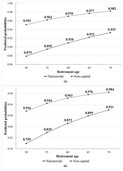
Figure 1. Predicted probabilities of owning a house for retirement age by region: (a) All retirees; (b) Late retirement group.

4.3. Housing Consumption of Retirees

In accordance with the empirical design, the relationships between retirement age and the consumption for housing services were finally tested by retirement group and region, after controlling for each retired household’s propensity of home ownership (Table 10, Table 11 and Table 12). From the Breusch–Pagan tests for heteroskedasticity, we could not reject the null hypothesis that the error terms are homoscedastic for all regressions, so we did not estimate robust standard errors for the predictors. The adjusted R² figures range from around 0.45 to 0.51, suggesting that the limited sets of variables in this study were satisfactorily selected, without causing further multicollinearity problems.

Table 10. Housing consumption (whole sample).

	Whole Sample		Subsample: Capital Region		Subsample: Non-Capital Region
Variables	Coeff.	S.E.	Coeff.	S.E.	Coeff.	S.E.
OWNPROB	0.0124 ***	0.001	0.0136 ***	0.002	0.0105 ***	0.001
AGE	−0.0017	0.002	0.0001	0.004	−0.0022	0.003
AGERE	−0.0079 ***	0.002	0.0007	0.004	−0.0094 ***	0.003
MSTATUS	−0.6779 ***	0.034	−0.7338 ***	0.067	−0.6415 ***	0.038
NETINC	0.0282	0.021	0.0183	0.031	0.0329	0.030
NETASSET	0.0032 ***	0.001	0.0021	0.002	0.0047 ***	0.001
APT	−0.0373	0.033	−0.0358	0.057	−0.0669 *	0.040
CAPITAL	0.1338 ***	0.040
Constant	3.7899 ***	0.181	3.2260 ***	0.384	4.0458 ***	0.205
Breusch–Pagan test for heteroskedasticity
Chi2	0.98		0.49		0.60
Prob > Chi2	0.3229		0.4828		0.4403
N	780		229		551
Adjusted R2	0.4482		0.4878		0.4330

* p < 0.1, *** p < 0.01.

Table 11. Housing consumption (early retirees).

	Early Retirement Group		Subsample: Capital Region		Subsample: Non-Capital Region
Variables	Coeff.	S.E.	Coeff.	S.E.	Coeff.	S.E.
OWNPROB	0.0091 ***	0.002	0.0053 **	0.002	0.0102 ***	0.002
AGE	−0.0009	0.004	−0.0042	0.007	0.0030	0.006
AGERE	−0.0128	0.012	−0.0228	0.020	0.0012	0.015
MSTATUS	−0.5749 ***	0.070	−0.5628 ***	0.106	−0.6045 ***	0.091
NETINC	0.0015	0.057	0.1401	0.092	−0.0261	0.071
NETASSET	0.0055 **	0.003	0.0077 **	0.003	0.0074 *	0.004
APT	−0.0186	0.067	0.1911 *	0.105	−0.1279	0.086
CAPITAL	−0.0735	0.080
Constant	4.1750 ***	0.678	4.9240 ***	1.165	3.0964 ***	0.870
Breusch–Pagan test for heteroskedasticity
Chi2	0.01		0.20		0.00
Prob > Chi2	0.9218		0.6523		0.9635
N	164		57		107
Adjusted R2	0.4413		0.5013		0.4614

* p < 0.1, ** p < 0.05, *** p < 0.01.

Table 12. Housing consumption (late retirees).

	Late Retirement Group		Subsample: Capital Region		Subsample: Non-Capital Region
Variables	Coeff.	S.E.	Coeff.	S.E.	Coeff.	S.E.
OWNPROB	0.0133 ***	0.001	0.0143 ***	0.003	0.0098 ***	0.001
AGE	−0.0014	0.003	0.0055	0.006	−0.0044	0.003
AGERE	−0.0115 ***	0.003	−0.0033	0.006	−0.0093 **	0.004
MSTATUS	−0.7136 ***	0.039	−0.7684 ***	0.085	−0.6526 ***	0.043
NETINC	0.0362	0.023	0.0266	0.035	0.0456	0.034
NETASSET	0.0029 **	0.001	0.0034	0.003	0.0046 ***	0.001
APT	−0.0460	0.038	−0.1377 *	0.070	−0.0541	0.046
CAPITAL	0.2010 ***	0.047
Constant	3.9565 ***	0.240	3.0903 ***	0.579	4.2656 ***	0.269
Breusch–Pagan test for heteroskedasticity
Chi2	1.01		1.66		0.67
Prob > Chi2	0.3156		0.1971		0.4127
N	616		172		444
Adjusted R2	0.4447		0.4759		0.4187

* p < 0.1, ** p < 0.05, *** p < 0.01.

All regressions suggest that the likelihood of having a home increases the level of housing consumption. The sample of the late retirement group for the capital region exhibits the highest effect (0.0143), meaning that a 1 percent point increase in the probability of home ownership leads to a 1.44 percent increase in dwelling size ($100\times \left[\exp \left(0.0143\right)-1\right]=1.44\%)$ for the retirees who retired at the age of 60 or later living in the non-capital region. It is worth noting that none of the AGE variables exert significant impacts on the dwelling size across different retiree groups and regions. The marital status (MSTATUS) variables are negatively associated with the dwelling size in all regressions. As the dependent variable is the living area per person, retired households with two persons consume less dwelling area per person than those with one-person households. While the coefficients for net asset (NETASSET) variables are positive and significant in some subsamples, those for net income turned out to be irrelevant to the variation of housing consumption.

The retirement age (AGERE) variables are negatively associated with the consumption for housing in the following samples: (i) the all-retiree sample for the whole country; (ii) the non-capital region for the entire retirement group; (iii) the late retirement group sample for the whole country; (iv) the late retirement group sample for the non-capital region. Therefore, we can conclude that later retirement results in a higher degree of economizing on housing consumption.

Finally, Table 13 reports the percentage change in the housing consumption of retirees for a one-unit and five-unit increase in the retirement age. For example, the coefficient of the retirement age variable for the entire retirement group for the whole country is −0.0079, so the consumption for housing decreases by about 0.787 percent as the retirement age increases by one year ($100\times \left[\exp \left(-0.0079\right)-1\right]=-0.787\%)$. The effect becomes −3.873 percent when the retirement age increases by five years ($100\times \left[\exp \left(-0.0079\times 5\right)-1\right]=-3.873\%$. As the retired household’s average dwelling size is 54.02 m² per person for all retirees nationwide (shown in Table 3), the amount of housing consumption per person for this group on average is expected to decrease by 0.43 m² if retirement occurs one year later, ending up with the dwelling size of 53.6 m². A five-year delay in retirement is associated with a decrease in housing consumption of 2.1 m² per person, and the resulting level of housing consumption becomes 51.9 m² per person.

Table 13. Effects of retirement age on housing consumption.

Sample	Region
	Nationwide	Capital	Non-Capital
Panel A: 1 year-increase in retirement age
All retirees	−0.787%	n.a. 1	−0.936%
Early retirement group	n.a.	n.a.	n.a.
Late retirement group	−1.143%	n.a.	−0.926%
Panel B: 5 year-increase in retirement age
All retirees	−3.873%	n.a.	−4.591%
Early retirement group	n.a.	n.a.	n.a.
Late retirement group	−5.588%	n.a.	−4.544%

¹ The effects are not reported here because the corresponding coefficients are not statistically significant at the alpha level of 0.05.

The magnitude of the economization of housing consumption for one-unit increase in the retirement age for all retirees is greater for the non-capital area than for the entire nation (0.936 percent versus 0.787 percent in terms of absolute values, respectively). As the effects are broken down into subsamples in regard to the timing of retirement, the late retiree group shows a higher degree of sensitivity of retirement timing to the adjustment for housing consumption for the entire nation (1.143 percent versus 0.787 percent in terms of absolute values, respectively). For the non-capital region, the effect for all retirees is greater than that for the late retirement group (0.936 percent versus 0.926 percent in terms of absolute values, respectively). The early retirement group does not show any impact of retirement timing on housing consumption adjustment. This irrelevance between retirement age and dwelling size also applies to the retired households living in the capital region.

5. Discussion

5.1. Housing Downsizing and Retirement-Consumption Puzzle

Downsizing homes is defined as “a residential move to smaller quarters and the necessary reduction of personal possessions” [70]. This study provides cross-section evidence that housing consumption by retired households decreases with the age of retirement, supporting the hypothesis of housing downsizing. However, our analysis, in terms of housing downsizing, shows different results when we segment the analysis by retirement group and region: Retired households in the capital region and in the early retirement group do not show the downsizing pattern. Therefore, our results do not follow the notion by Fisher et al. [14], which suggests that early retirement induces a higher degree of liquidation of housing wealth than late retirement.

Our results are partly in line with the so-called “retirement-consumption puzzle” with respect to housing consumption. According to the life-cycle hypothesis, even though income discontinuously decreases with retirement, consumption should not be significantly different from the pre-retirement level with respect to lifetime utility maximization and the resulting consumption smoothing. However, some studies found that, in the case of retired households, not only the income level, but also the consumption level, decreases compared to that before retirement. This phenomenon has been referred to as the retirement-consumption puzzle because it is not satisfactorily explained by the permanent income hypothesis that forms the theoretical basis in exploring household consumption behavior. There are various opinions on what the cause is, to what extent the decline occurs, or whether the phenomenon is common to all retirement groups or specific to certain groups or consumption items.

The paper by Hamermech [71] is a pioneering study presenting evidence on the relationship between consumption and assets using the US Retirement History Survey (RHS). The study found that the average consumption of households in their early retirement period exceeded their income level by about 14%. Furthermore, it was found that these households increased their net financial wealth by sharply reducing the level of consumption within a short period of time after retirement. This means that, if it is difficult to maintain the level of consumption enjoyed at the beginning of retirement because their assets are insufficient, their real consumption is reduced in order to cover the gap. A study by Bank et al. [72] analyzed income and expenditure patterns before and after retirement by retirement age cohort, using the British Family Expenditure Survey data, to explore whether households are saving enough for retirement. The results show that there was a significant decrease in consumption around the time of retirement, which was different from the consumption smoothing framework. Even after taking into account job-related expenses, changes in consumption that may be related to the risk of death, and other determinants, the consumption decline predicted by the model was about 2 percent, while the actual consumption decline in the retirement period was 3 percent. The authors concluded that this behavior results from the decrease in consumption due to unexpected negative shocks. Bernheim et al. [73] also reported similar results. This study estimated consumption patterns for the Panel Study of Income Dynamics (PSID) for 430 households between 1978 and 1990. The authors found that consumption decreased by 14 percent on average at the time of retirement. They interpreted the rapid decline in consumption at the time of retirement as an action taken by households after inspecting their retirement preparation status. It could be the case that those households reduce consumption in response to future negative shocks.

The puzzle is pertinent to housing. According to the life-cycle hypothesis suggested by Ando and Modigliani [74], households withdraw accumulated financial and housing assets for consumption after retirement. Therefore, they increase housing assets when they are young, and reduce those assets when they are getting older. However, there are studies that have tried to modify or refute existing predictions by the life-cycle model related to housing when it comes to the changes in residential status of middle-aged households. Although it has been recognized that older households retain large housing assets and their income levels cannot satisfactorily cover household expenditures, alternative hypotheses have suggested that the possibility of downsizing housing is low if demographic shocks, such as death, illness, or divorce, do not occur, or if people want their children to inherit the housing assets. Beblo and Schreiber [75] found that the strict consumption-smoothing hypothesis is violated for the subgroup of non-home owners for German tenants. Even though our study cannot identify the exact reasons, the results suggest that consumption for housing after retirement discontinuously declines. In other words, a decline in housing consumption does not occur through the entire time path after retirement in a smooth way: the reduction in housing consumption does not happen in early retirement, but in late retirement.

5.2. Housing Policy Recommendations

As the retirement of the baby boomers begins, much attention is being paid to the prediction that older households put their homes on the market through downsizing. In Korea, retiring households’ income sources are rapidly decreasing, in part due to the immaturity of public and private pension systems. It is argued that housing represents a high proportion of household assets, and there are relatively few liquid assets that can be used for daily consumption [26]. According to the Korea Housing Finance Corporation [76], 30 percent of the elderly, who own their own homes, had accumulated debts of about KRW 44 million; 20% covered their monthly expenditures with public pensions, such as the national pension, and 40.9% answered that their average income is insufficient.

A reverse mortgage system enables the elderly who own a house to receive a stable monthly income through liquidating housing wealth in the form of a pension. In July 2007, the Korea Housing Finance Corporation launched a reverse mortgage program called “Housing Pension” for the purpose of alleviating the problems of public and private pensions, which are thought to be inefficient in coping with the trend of a rapidly aging society. However, the subscription rate is still low. According to the Korea Housing Finance Corporation, as of January 2017, the 10th year since its inception, the number of subscribers is 40,586. This is less than 1% of 4,969,773 people, which is the population of those aged 60 or older, as of the 2015 Population and Housing Census. The reasons for the low rate include house bequest motivation, expectations for house price appreciation, and the low level of receivable income from the program [77].

The poverty rate of the elderly aged 65 or older in Korea is 43.8%, which is more than triple the average of 14.0% in OECD members [78]. South Korea has a high population density around its capital, which causes housing costs to continuously rise around the area. Therefore, it is difficult for retirees who generally have a relatively low income to own a house in the urban area [79,80]. It turns out that the elderly living in the Seoul metropolitan area are more satisfied with reverse mortgages than the elderly living in non-Seoul areas, as they use such mortgages to cover their relatively high living expenses in the highly dense area [77]. It is thus necessary for the reverse mortgage program to be redesigned, to be expanded, or to be made more accessible to those who retire earlier in the capital region because some retired households might over-consume housing involuntarily [62]. Another concern arises: the reverse mortgage program only supports older home owners. As for the renters, we need to devise policy measures to lower the rental costs, such as the provision of public housing or direct assistance, that are tailored to those who did not accumulate enough housing wealth to prepare for the later stage of life or to those who experience difficulty moving to a smaller housing unit in the rental housing market.

6. Concluding Remarks

This paper has investigated the impact of the timing of retirement on housing consumption. Incorporating the endogeneity of housing tenure choice, this study found that households whose household heads retire at the age of 60 or later living in the non-capital region exhibit a negative relationship between the age of retirement and the level of housing consumption, which corresponds to housing downsizing. On the other hand, the early retirement group living in the more populated region does not downsize their house. If the differential impacts of the timing of retirement on housing consumption indicate that the elderly who retire early in the capital region have difficulty reducing their dwelling size in a timely manner, housing policies should pay more attention to revising the current reverse mortgage program or assisting renters through a combination of direct support and the supply of affordable housing.

Three limitations should be addressed. First, we only used the SFLC dataset for one year (2014) because Statistics Korea provides the dwelling size variable as discrete, not continuous, starting from the 2015 dataset, for the sake of increasing confidentiality. As a result, we could not obtain a sufficient number of cases, especially for the early retirement group. Second, we could not add the price variable in the housing consumption regression. We need to estimate the user cost of owning, the rent, and the ratio of those two (the relative price). We could not observe both the value and rent for each observation. In addition, in order to estimate those metrics, we need detailed information on the variables for the hedonic pricing model. The data used in this study lack such information. Finally, because of the limited usability of the data, we could not construct the data as a longitudinal dataset, which has advantages over the one-year data in that we could capture the changes in the retirement status from repeated observations and compare them with the changes of housing consumption. However, given some of the difficulties in using the data, our approach and the results shed some light on the impact of the timing of retirement on housing consumption. We look forward to more studies that examine the spatial heterogeneity of the housing downsizing behaviors for different retirement groups and derive relevant housing policy directions.

References

- National Institute of Population and Social Security Research (NIPSSR). Latest Demographic Statistics; Population Research Series No. 333; NIPSSR: Tokyo, Japan, 2015. [Google Scholar]
- Statistics Korea. 2016 Statistics on the Aged; Statistics Korea: Sejong, Korea, 2016.
- Beehr, T.A.; Glazer, S.; Nielson, N.L.; Farmer, S.J. Work and nonwork predictors of employees’ retirement ages. J. Vocat. Behav. 2000, 57, 206–225. [Google Scholar] [CrossRef]
- Cremer, H.; Lozachmeur, J.-M.; Pestieau, P. Social security, retirement age and optimal income taxation. J. Public Econ. 2004, 88, 2259–2281. [Google Scholar] [CrossRef]
- Statistics Korea. The Survey of Household Finances and Living Conditions (SFLC) in 2014; Statistics Korea: Sejong, Korea, 2014.
- Bottazzi, R.; Jappelli, T.; Padula, M. Retirement expectations, pension reforms, and their impact on private wealth accumulation. J. Public Econ. 2006, 90, 2187–2212. [Google Scholar] [CrossRef]
- Maestas, N. Back to work expectations and realizations of work after retirement. J. Hum. Resour. 2010, 45, 718–748. [Google Scholar] [CrossRef]
- Van der Klaauw, W.; Wolpin, K.I. Social security and the retirement and savings behavior of low-income households. J. Econom. 2008, 145, 21–42. [Google Scholar] [CrossRef]
- Statistics Korea. 2017 Statistics—Elderly Population; Statistics Korea: Sejong, Korea, 2017.
- Baek, E.Y.; Joung, S.H. Baby boomers’ financial status and the effects of housing equity on retirement preparation. J. Consum. Cult. 2012, 15, 141–160. (In Korean) [Google Scholar]
- Choi, H.B.; Lee, J.S.; Choi, Y. An Analysis on the Determinants of Real Estate Assets Management of the Retiree. Korea Real Estate Acad. Rev. 2016, 65, 146–160. (In Korean) [Google Scholar]
- Won, S.J.; Song, I.U. Factors Affecting Perceived Retirement Preparation of Babyboomers in Gyeongbuk Province. J. Rural Soc. 2014, 24, 85–112. (In Korean) [Google Scholar]
- Munnell, A.H.; Sass, S.A. The Decline of Career Employment; Issues in Brief ib2008-8-14; Center for Retirement Research at Boston College: Chestnut Hill, MA, USA, 2008. [Google Scholar]
- Fisher, G.G.; Chaffee, D.S.; Sonnega, A. Retirement timing: A review and recommendations for future research. Work. Retire. 2016, 2, 230–261. [Google Scholar] [CrossRef]
- Gunderson, M.; Riddell, W. Labour Market Economics; McGraw-Hill Ryerson: Toronto, ON, Canada, 1993. [Google Scholar]
- Burtless, G.; Moffitt, R. (Eds.) The effect of social security benefits on the labor supply of the aged. In Retirement and Economic Behavior; Brookings Institution: Washington, DC, USA, 1984; pp. 135–171. [Google Scholar]
- Shin, J.H.; Choi, M.J. Reallocation of real estate assets of the retiree in Korea and its influencing factors. J. Korea Plan. Assoc. 2013, 48, 201–212. (In Korean) [Google Scholar]
- Barfield, R.E.; Morgan, J.N. Early Retirement: The Decision and the Experience; Survey Research Center, University of Michigan: Ann Arbor, MI, USA, 1969. [Google Scholar]
- Han, H.J.; Kang, E.S. Changes of life condition after retirement. J. Korean Acad. Psychiatr. Ment. Health Nurs. 2001, 10, 203–219. (In Korean) [Google Scholar]
- Kweon, M.I. Determinants of retirement and post-retirement work behavior of older Koreans. Korean J. Soc. Welf. Stud. 1996, 8, 41–67. (In Korean) [Google Scholar]
- Morse, D.; Dutka, A.B.; Gray, S.H. Life after Early Retirement: The Experiences of Lower-Level Workers; Rowman & Littlefield Pub Inc.: Lanham, MD, USA, 1983. [Google Scholar]
- Fields, G.S.; Mitchell, O.S. Retirement, Pensions, and Social Security; MIT Press: Cambridge, MA, USA, 1984. [Google Scholar]
- Kim, J.-Y.; Chang, Y.-G. A study on the asset management utilizing real estate for the retired households. Hous. Stud. Rev. 2012, 20, 125–155. (In Korean) [Google Scholar]
- Parnés, H.S.; Adams, A.; Andrisani, P.; Kohlen, A.; Nestel, G. The Pre-Retirement Years: Five Years in the Work Lives of Middle-Age Men; Center for Human Resource Research: Columbus, OH, USA, 1974. [Google Scholar]
- OECD. Working Better with Age: Korea; OECD Publishing: Paris, France, 2018. [Google Scholar]
- Kim, Y.-J.; Son, J.-Y. Determinants of Housing Downsizing among the Older Homeowners. Hous. Stud. Rev. 2014, 22, 29–57. (In Korean) [Google Scholar]
- Szinovacz, M.E.; Martin, L.; Davey, A. Recession and expected retirement age: Another look at the evidence. Gerontol. 2014, 54, 245–257. [Google Scholar] [CrossRef] [PubMed]
- Coile, C.C.; Levine, P.B. The market crash and mass layoffs: How the current economic crisis may affect retirement. Be J. Econ. Anal. Policy 2011, 11. [Google Scholar] [CrossRef]
- Goda, G.S.; Shoven, J.B.; Slavov, S.N. What explains changes in retirement plans during the Great Recession? Am. Econ. Rev. 2011, 101, 29–34. [Google Scholar] [CrossRef]
- Farnham, M.; Sevak, P. Housing Wealth and Retirement Timing; Paper No. UM WP, 172; Michigan Retirement Research Center: Ann Arbor, MI, USA, 2007. [Google Scholar]
- Hartig, T.; Fransson, U. Housing tenure and early retirement for health reasons in Sweden. Scand. J. Public Health 2006, 34, 472–479. [Google Scholar] [CrossRef]
- Gorodnichenko, Y.; Song, J.; Stolyarov, D. Macroeconomic Determinants of Retirement Timing; NBER Working Paper No. 19638; National Bureau of Economic Research: Cambridge, MA, USA, 2013. [Google Scholar]
- Disney, R.; Ratcliffe, A.; Smith, S. Booms, busts and retirement timing. Economica 2015, 82, 399–419. [Google Scholar] [CrossRef]
- Kim, K.; Jeon, J.S. Why do households rent while owning houses? Housing sub-tenure choice in South Korea. Habitat Int. 2012, 36, 101–107. [Google Scholar] [CrossRef]
- Lin, Y.-J.; Chang, C.-O.; Chen, C.-L. Why homebuyers have a high housing affordability problem: Quantile regression analysis. Habitat Int. 2014, 43, 41–47. [Google Scholar]
- Disney, R.; Johnson, P.; Stears, G. Asset wealth and asset decumulation among households in the Retirement Survey. Fisc. Stud. 1998, 19, 153–174. [Google Scholar]
- Benjamin, J.; Chinloy, P.; Jud, D. Why do households concentrate their wealth in housing? J. Real Estate Res. 2004, 26, 329–344. [Google Scholar]
- Blanco, A.; Gilbert, A.; Kim, J. Housing tenure in Latin American cities: The role of household income. Habitat Int. 2016, 51, 1–10. [Google Scholar]
- Lee, C.-C.; Ho, Y.-M.; Chiu, H.-Y. Role of personal conditions, housing properties, private loans, and housing tenure choice. Habitat Int. 2016, 53, 301–311. [Google Scholar]
- Chiu, R.L.; Ho, M.H. Estimation of elderly housing demand in an Asian city: Methodological issues and policy implications. Habitat Int. 2006, 30, 965–980. [Google Scholar]
- Sinai, T.; Souleles, N.S. Owner-occupied housing as a hedge against rent risk. Q. J. Econ. 2005, 120, 763–789. [Google Scholar]
- Hirayama, Y. The role of home ownership in Japan’s aged society. J. Hous. Built Environ. 2010, 25, 175–191. [Google Scholar]
- Flavin, M.; Yamashita, T. Owner-occupied housing and the composition of the household portfolio. Am. Econ. Rev. 2002, 92, 345–362. [Google Scholar]
- Li, W.D. Households’ movements and the private rented sector in Taiwan. Habitat Int. 2008, 32, 74–85. [Google Scholar]
- Marais, L.; Cloete, J. Financed homeownership and the economic downturn in South Africa. Habitat Int. 2015, 50, 261–269. [Google Scholar] [CrossRef]
- Tu, Y.; Kwee, L.K.; Yuen, B. An empirical analysis of Singapore households’ upgrading mobility behaviour: From public homeownership to private homeownership. Habitat Int. 2005, 29, 511–525. [Google Scholar] [CrossRef]
- Chiuri, M.C.; Jappelli, T. Do the elderly reduce housing equity? An international comparison. J. Popul. Econ. 2010, 23, 643–663. [Google Scholar] [CrossRef]
- Banks, J.; Blundell, R.; Oldfield, Z.; Smith, J.P. Housing Price Volatility and Downsizing in Later Life; NBER Working Paper No. 13496; National Bureau of Economic Research: Cambridge, MA, USA, 2007. [Google Scholar]
- Yogo, M. Portfolio choice in retirement: Health risk and the demand for annuities, housing, and risky assets. J. Monet. Econ. 2016, 80, 17–34. [Google Scholar] [CrossRef] [PubMed]
- Crossley, T.F.; Ostrovsky, Y. A Synthetic Cohort Analysis of Canadian Housing Careers; Social and Economic Dimensions of an Aging Population Research Papers, no. 107; McMaster University: Hamilton, ON, Canada, 2003. [Google Scholar]
- Ermisch, J.F.; Jenkins, S.P. Retirement and housing adjustment in later life: Evidence from the British Household Panel Survey. Labour Econ. 1999, 6, 311–333. [Google Scholar] [CrossRef]
- Feinstein, J.; McFadden, D. The dynamics of housing demand by the elderly: Wealth, cash flow, and demographic effects. In The Economics of Aging; Wise, D.A., Ed.; University of Chicago Press: Chicago, IL, USA, 1989; pp. 55–92. [Google Scholar]
- Munnell, A.H.; Soto, M.; Aubry, J.-P. Do People Plan to Tap Their Home Equity in Retirement? Center for Retirement Research at Boston College: Chestnut Hill, MA, USA, 2007. [Google Scholar]
- Venti, S.F.; Wise, D.A. Aging and Housing Equity; NBER Working Paper, No. 7882; National Bureau of Economic Research: Cambridge, MA, USA, 2000. [Google Scholar]
- Venti, S.F.; Wise, D.A. Aging and housing equity: Another look. In Perspectives on the Economics of Aging; Wise, D.A., Ed.; University of Chicago Press: Chicago, IL, USA, 2004; pp. 9–48. [Google Scholar]
- Artle, R.; Varaiya, P. Life cycle consumption and homeownership. J. Econ. Theory 1978, 18, 38–58. [Google Scholar] [CrossRef]
- Jones, L.D. The tenure transition decision for elderly homeowners. J. Urban. Econ. 1997, 41, 243–263. [Google Scholar] [CrossRef]
- Venti, S.F.; Wise, D.A. Aging, moving, and housing wealth. In The Economics of Aging; Wise, D.A., Ed.; University of Chicago Press: Chicago, IL, USA, 1989; pp. 9–54. [Google Scholar]
- Jeong, W.Y.; Lee, H.S. Financial structures of real estate and the factors influencing on it by subjective financial adequacy for later years among middle & old aged households. J. Korean Home Econ. Assoc. 2010, 48, 1–12. [Google Scholar]
- Kim, J.-Y.; Jeong, J.H. The Effects of Housing Wealth on the Balance of Elderly Household Accounts. J. Econ. Geogr. Soc. Korea 2012, 15, 534–549. (In Korean) [Google Scholar]
- Ko, J.; Kim, J.-H.; Kang, M.-G. Housing wealth transfer behavior among the middle-aged and older households in Seoul. Seoul Stud. 2015, 16, 41–55. (In Korean) [Google Scholar]
- Clark, W.A.; Deurloo, M.C. Aging in place and housing over-consumption. J. Hous. Built Environ. 2006, 21, 257–270. [Google Scholar] [CrossRef]
- King, M.A. An econometric model of tenure choice and demand for housing as a joint decision. J. Public Econ. 1980, 14, 137–159. [Google Scholar] [CrossRef]
- Goodman, A.C. An econometric model of housing price, permanent income, tenure choice, and housing demand. J. Urban. Econ. 1988, 23, 327–353. [Google Scholar] [CrossRef]
- Ahmad, N. A joint model of tenure choice and demand for housing in the city of Karachi. Urban. Stud. 1994, 31, 1691–1706. [Google Scholar] [CrossRef]
- Fan, Y.; Yavas, A. How does mortgage debt affect household consumption? Micro evidence from China. Real Estate Econ. 2020, 48, 43–88. [Google Scholar] [CrossRef]
- Kim, H. Private Income Transfers and Old-Age Income Security. Kdi J. Econ. Policy 2008, 30, 71–130. (In Korean) [Google Scholar]
- Korea Research Institute for Human Settlements (KRIHS). Retirement of Baby Boom Generation and the Strategy for Revitalization of Rural Areas in Korea; Korea Research Institute for Human Settlements: Sejong, Korea, 2011. (In Korean) [Google Scholar]
- Lim, M.-H. A Study on the Influence Factors on Residential Mobility Plan to Non-Capital Area of Households in Capital Area. Hous. Stud. Rev. 2019, 27, 117–134. (In Korean) [Google Scholar] [CrossRef]
- Luborsky, M.R.; Lysack, C.L.; Van Nuil, J. Refashioning one’s place in time: Stories of household downsizing in later life. J. Aging Stud. 2011, 25, 243–252. [Google Scholar] [CrossRef] [PubMed]
- Hamermesh, D.S. Life-cycle effects on consumption and retirement. J. Labor Econ. 1984, 2, 353–370. [Google Scholar] [CrossRef]
- Banks, J.; Blundell, R.; Tanner, S. Is there a retirement-savings puzzle? Am. Econ. Rev. 1998, 88, 769–788. [Google Scholar]
- Bernheim, B.D.; Skinner, J.; Weinberg, S. What accounts for the variation in retirement wealth among US households? Am. Econ. Rev. 2001, 91, 832–857. [Google Scholar] [CrossRef]
- Ando, A.; Modigliani, F. The “Life-Cycle” Hypothesis of Saving: Aggregate Implications and Tests. Am. Econ. Rev. 1963, 53, 55–84. [Google Scholar]
- Beblo, M.; Schreiber, S. The Life-Cycle Hypothesis Revisited: Evidence on Housing Consumption after Retirement; SOEPpaper No. 339; Deutsches Institut für Wirtschaftsforschung: Berlin, Germany, 2010. [Google Scholar]
- Korea Housing Finance Corporation (HF). 2012 Housing Pension Demand Survey; Korea Housing Finance Corporation (HF): Busan, Korea, 2013. [Google Scholar]
- Lee, J.S.; Choi, Y. A Study on Determinants of Use and Satisfaction of Reverse Mortgage Considering Socioeconomic Characteristics of the Elderly. J. Korean Soc. Civ. Eng. 2017, 37, 437–444. (In Korean) [Google Scholar] [CrossRef]
- Choi, H.-S. A Numerical analysis to study whether the early termination of reverse mortgages is rational. Sustainability 2019, 11, 6820. [Google Scholar] [CrossRef]
- Kim, J.; Kim, K. Aging and Housing Market: Evidence from Changes in Housing Consumption Before and After Retirement. J. Korea Real Estate Anal. Assoc. 2011, 17, 59–71. (In Korean) [Google Scholar]
- Lee, M.-H.; Jang, Y.-J. An empirical study on the household income inequality and its determinants in Korea. J. Ind. Innov. 2011, 27, 111–138. (In Korean) [Google Scholar]
Publisher’s Note: MDPI stays neutral with regard to jurisdictional claims in published maps and institutional affiliations. |
© 2021 by the authors. Licensee MDPI, Basel, Switzerland. This article is an open access article distributed under the terms and conditions of the Creative Commons Attribution (CC BY) license (http://creativecommons.org/licenses/by/4.0/).