Abstract
Resource tax has been widely adopted in many countries. This paper evaluates the causal effect of reform of water resources tax on water resources performance in Hebei Province, China. By using the provincial panel data, we first measure the water resources performance of 21 provinces from 2008 to 2018 by considering the NDDF-ML method of undesirable output. We found that each province in China has gradually improved its water resources performance in the past 10 years, but there are great differences between regions. Then, we employ the synthetic control method, which allows us to consider the influence of unobservable time-varying factors to evaluate the policy effect. The results show that water performance index has increased significantly by 18.0%. The effect is mainly due to technological progress (17.3%) rather than technological efficiency (0.7%), which means no significant improvement in the allocation of water, and after placebo tests, our results are still robust. The DID approach shows a similar conclusion, but unobservable time-variation caused by other policies may lead to an overestimation of DID. In order to make good use of water resources, China should accelerate the reform of water resource taxes and pay more attention to the allocation of water resources.
1. Introduction
Water resources are the basic conditions for maintaining people’s lives and promoting economic development. Environmental pollution and unpredictable climate change further exacerbate water scarcity problems [1,2], particularly in developing countries characterized by rapid population growth and rapid urbanization [3]. China’s per capita water resources are far below the world average, about one-fourth of the average, one of the most water-deficient countries in the world. In addition, the distribution of water resources in various regions is very uneven. The land area of the Yangtze River Basin and its south area accounts for only 36.5 percent of the country, and its water resources account for an exacerbated 81 percent of the country. With the progress of social and economic development, the process of urbanization continues to accelerate, and domestic and industrial water consumption has increased significantly. Water pollution exacerbates the problem of drinking water supply shortage. For example, the Yangtze River is a drinking water source for 800 million people, and it undertakes the most serious industrial activities of water pollution in China [4]. Due to water pollution, about 190 million people become sick and 60,000 people die every year [5]. Rapid urbanization and economic growth have created a large demand for water resources [6,7]. In order to meet the needs of life and industrial development in water resources, the rational use of water resources and improvement of water efficiency are very important for the sustainable development of the economy and society in China.
China’s extensive economic growth model depends on a large consumption of resources and energy, which leads to pollution and low efficiency. For observing the performance of resource utilization under environmental constraints, it is necessary to integrate resource factor input and environmental economic output into the evaluation framework. As a nonparametric method, data envelopment analysis can be used to evaluate the performance of a multi-input–output decision unit based on relative efficiency [8]. Since the form of a production function is not assumed in advance, the evaluation of the decision unit will be more objective. The Malmquist–Luenberger productivity index can also measure the relative position change (efficiency change) of the production unit and the production front by constructing the optimal actual production front, as well as the movement of the production front itself (technological progress) [9].
Chinese government announced water resources tax reform (WRTR) in Hebei Province in 2016. Choosing it as a pilot province may be due to many reasons. In order to avoid the strong endogeneity of the policy, we are concerned about the effect on Hebei Province, which is the only one province. In this paper, the synthetic control method [10,11] is introduced to estimate the impact of Hebei’s water resources tax reform on water efficiency. Synthetic control improves the limitation of traditional policy evaluation methods and creates a new method of constructing counterfactuals. The basic idea is that, though it is difficult to find a control group that is highly similar to the treatment group, a highly similar “synthetic Hebei” can be constructed by making appropriate linear combinations of provinces that have not implemented water resources tax reform. The gap between “real Hebei” and “synthetic Hebei” in water performance can be regarded as the effect of water resource tax reform.
The pilot of WRTR in December 2017 expanded to nine provinces, including Beijing and Tianjin. The water efficiency of these nine provinces is also affected by this policy later, and they are not suitable to be included in control group. In order to accurately reflect the effect of WRTR in Hebei Province, the control group of this paper only includes 21 other provinces that have not implemented the WRTR pilot between 2008 and 2018 (except the 9 provinces we mentioned above, Hong Kong, Macao, Taiwan, and Tibet). The input indicators include fixed assets investment, social labor force, and total water use, and the output indicators include regional GDP and chemical oxygen demand (COD) emissions. Firstly, considering the undesirable output, the environmental technical efficiency of water resources utilization in China is evaluated (based on 2007), and the data envelopment analysis method is used to measure the water resources efficiency of provincial regions. After that, the synthetic control method (SCM) is used to evaluate the effect of the policy, and then to provide policy suggestions for improving water resources efficiency and solving the problem of water resources shortage.
The first contribution of this paper is to determine the causal effects of WRTR policy and solve the problem of endogeneity related to WRTR. There may be unobservable factors with time-varying effects in each province, resulting in the difference in water resources performance. Even if the parallel trend is met before the implementation of the policy, some policies may interfere with the policy in the year of policy implementation because China also promulgated a number of water related policies in 2016. We used the synthetic control method, DID, and their robustness tests to verify. Secondly, this paper decomposes water resources performance and supplements the mechanism of WRTR affecting performance. When the cost of water increases, residents and enterprises can improve their awareness of water conservation by recycling, using more advanced equipment, or redistributing water resources in different departments. Therefore, this paper evaluates the overall performance of water resources and the policy’s causal effects on efficiency and technology.
Non-radial Malmquist Water Performance Index (NMWPI).
Our results show that the policy effect is positive and significant. After the implementation of WRTR, the non-radial Malmquist water performance index (NMWPI) increased significantly that year, with an average increase of 18.0% during post-treatment. It was found that the technical change (TC) increased by 17.3% and the efficiency technology (EC) only increased by 0.7%; the change trends of NMWPI and TC are similar, while the causal effect of EC is weak and insignificant; and TC is the main driving factor of NMWPI. Finally, the DID approach found similar results, which proves the robustness of our results again.
The structure of this paper is as follows: Section 2 describes the implementation background of water resources tax policy. Section 3 is the introduction of research methods. Section 4 is the selection of data and variables used in this paper. Section 5 is the measurement results of water resources performance, and the empirical analysis of the impact of water resources tax on water resources performance by using the synthetic control method. The fifth part summarizes the research and puts forward some suggestions.
2. Policy Background
The collection of taxes and fees on water resources is a common method. Many countries in Europe have adopted water resources tax laws to clarify the tax obligations of water users or consumers in order to save water resources and improve the efficiency of water resources utilization. In 1970, the Netherlands adopted and enacted the Surface Water Pollution Act to prevent groundwater depletion from the over-exploitation of groundwater resources. The Groundwater Act was passed in 1981, and a groundwater tax was introduced in 1995. France introduced a water pollution tax in 1968 and a water resources tax in 1996. Denmark introduced a tap water tax in 1994, as part of Denmark’s green tax reform, which is essentially similar to the groundwater tax, since almost all Danish drinking water originates underground. Although Russia is rich in water resources, there are problems of regional distribution imbalance and water quality pollution. In order to manage water resources effectively, the tax law of the Russian Federation, which began in 2005, stipulates the specific contents of the collection and management of the water resources tax. In China, the collection of water resources fees began in the early 1980s, when cities began to set fees system, and continues to improve. However, due to the lack of uniform legal provisions, the charge standards of water fees were often formulated by local governments. Therefore, there are great differences in the charge standards of water resources fees in different regions, and even some governments exempt some high-polluting enterprises from water resources fees for economic development. This difference is obviously not conducive to strengthening water resources management by means of taxes and fees. On 10 May 2016, the Ministry of Finance and the State Administration of Taxation jointly issued a circular on comprehensively promoting the reform of the resource tax, announcing that China would comprehensively promote the reform of the resource tax and carry out pilot work on the reform of the water resource tax as of 1 June 2016. Under the TFR or FGS (tax for fee or Fei Gai Shui) reform, various types of irregular fees abolished and replaced with a single water tax. In the past, there were unauthorized manipulations in government fund management [12]. Since 1994, China has implemented some important tax reforms, including an agricultural tax reform, a resource tax, and a property tax. These reforms are considered to be a possible way to solve the excessive financial plunder of local governments [13,14], that is, to reduce or prohibit the misappropriation of funds by local governments. The existing literature on FGS reform in China mainly focuses on the rural FGS reform, which started in 2001 [15,16,17,18]. Is a water resource tax better than a water resource fee? The research of different scholars has not reached a consistent conclusion. Chen et al. [18] found that a water resources tax reduces output by increasing the cost difference between enterprises, while a water resources fee reduces market scale and effects output. A water resources tax is more conducive to the elimination of backward enterprises. Ma et al. [19] believe that the tax system reform can reduce arbitrary charges and make the collection and use of water resources tax more reasonable and transparent. Zhao and Zhang [20] found that the water resources tax reform can reduce the water consumption per unit of industrial output value but has no significant impact on the total water consumption. Yang et al. [21] used the synthetic control method and found that water resources tax can reduce the water consumption per CNY 10000 of GDP and the total water consumption. Kennedy [22] argues that FGS reduces the financial capacity of local governments, resulting in the reduction of public services. Mushtaq et al. [12] found that FGS of water resources may hinder agricultural production.
Hebei is one of the few provinces in the country that has no major rivers passing through it, so water resources are seriously inadequate and water for economic and social development has had to rely on the over-exploitation of groundwater for a long time. From the perspective of per capita water resources, Hebei’s per capita water resources are 283 cubic meters, which is only one-seventh of the national per capita water resources, which is far lower than the internationally recognized “extreme water shortage standard” of 500 cubic meters per capita. From the comparison between Hebei’s per capita water resources and the national per capita water resources in the past 10 years, Hebei’s per capita water resources are only about one-tenth of the national level. In addition, economic development requires a large amount of water. The province’s total water shortage in general years is 12.43 billion cubic meters, of which 7.23 billion cubic meters of water is lacking for economic and social development and 5.2 billion cubic meters of water for the ecological environment. The “Administrative Measures for the Collection of Water Resources Taxes in Hebei Province” imposes differential tax rates on different water withdrawal behaviors in different industries. For example, higher tax standards imposed on the use of groundwater in over-extraction areas of groundwater and the use of water for special industries. This design embodies the restriction of groundwater exploitation and the restriction of high water consumption. This policy is China’s first attempt to use taxation to regulate the use of water resources and is of great significance to water resources management. The difference between a water fee and a water resource tax can be seen in Table 1.

Table 1.
Comparison of water resources fee and water resources tax.
3. Methodology
3.1. Non-Radial Distance Function Malmquist–Luenberger Index (NDDF-ML)
3.1.1. Input–Output Variables Measured by Water Resources Performance Non-Radial Distance Function (NDDF)
Data Envelopment Analysis (DEA) is a common tool for assessing energy and environmental efficiency performance. Methodologically, DEA is a linear programming model. Therefore, by assessing the distance between the decision making unit (DMU) and the boundary, its relative efficiency [23] can be easily determined. Conventional data envelopment analysis models are generally based on Shepherd distance functions. The Shepherd distance function expands the desirable output and the undesirable output in the same proportion [24]. This means that the reduction of undesirable outputs is not credible, and traditional data envelopment analysis models are limited in measuring energy and environmental efficiency. To solve this problem, Chung et al. [25] proposed the directional distance function (DDF) method. DDF distinguishes between strong and weak tractability between desirable and undesirable outputs. In addition, DDF allows for an increase in the desired output while reducing undesired outputs and inputs. Therefore, DDF is gradually applied to empirical research. However, its limitation is that the expansion of desirable outputs and the contraction of undesirable outputs/inputs are changed at the same rate [26]. In this sense, DDF is a measure of radial efficiency, and it may underestimate the inefficiency of the evaluated units. Given the limitations of the DDF approach, Zhou et al. [27] proposed a non-radial distance function (NDDF) method. In comparison, NDDF allows for different proportions of adjustments to inputs, desirable outputs, and undesirable outputs. Therefore, NDDF has higher recognition ability than DDF. Fukuyama and Weber [28] believe that the non-radial directional distance function (NDDF) can avoid input redundancy and make the calculated efficiency more accurate. Considering the advantages and characteristics of the NDDF, we applied it in this paper. Assuming there are N assessment areas, each region is regarded as a DMU, and each DMU uses capital (K), labor (L), and water resources (W) to produce desirable goods (Y). Meanwhile, undesired chemical oxygen demand (C) emissions are produced during production. According to the Färe et al.’s [29] joint production framework, production technologies may be expressed as:
Assuming that the production technology set has the following characteristics:
- (i)
- P is a bounded set, which means that limited inputs produce only limited outputs.
- (ii)
- If , , then . It is called zero combination, that is, if the expected output is produced, the unexpected output will also be produced
- (iii)
- If , then . This feature is called the strong disposability of inputs and desirable outputs, which means that inputs and expected outputs can be changed without constraints.
- (iv)
- If , , then . This situation is called weak disposability of undesirable output, which means that if we to reduce the undesired output, we must reduce the expected output.
With these assumptions, the production techniques used to describe the joint production of desirable output Y and undesirable output C have been conceptually well defined but cannot be directly used in empirical analysis. A common practice is to describe production techniques within a nonparametric framework, which can be performed using piecewise convex combinations (DEA) of observed data. Suppose there are provinces. For province i, inputs, desirable outputs, and undesirable outputs in provinces are , and the environmental production technologies that show constant returns to scale in N provinces can be described as follows:
According to Zhou et al. [27], Zhang et al. [30], and Zhang and Choi [24], non-radial distance functions are defined as:
where is the proportional factor vector that measures the deviation of actual production activity from the best state; represents the diagonal matrix; is a direction vector that determines the direction in which each input and output is scaled; and is a vector that represents the weight assigned to each input and output. Values of NDDF for specific province can be solved by the following DEA models:
Direction vector g and weight vector w can be set in different ways to serve different policy objectives. To evaluate China’s regional water resource utilization efficiency, we set the direction vector to , , which emphasizes water resources input, desirable output, and chemical oxygen demand (COD) emissions and eliminates the dilution effect of other inputs (capital and labor) because capital and labor do not directly produce emissions. Suppose that under and , is the solution of Equation (1). On the basis of Zhou et al. [27] and Zhang et al. [31], the total-factor water performance index (TWPI) can be described as follows:
Formula (5) measures the maximum possible increase in water resources utilization intensity, which can be used to measure the water resources performance of each province in a specific time period, and TWPI is between 0 and 1. In order to investigate the dynamic change in water resources’ performance over time, considering non-radial relaxation, we propose a water performance index for non-radial Malmquist in the next section (NMWPI).
3.1.2. Non-Radial Malmquist–Luenberger Water Performance Index
The Malmquist productivity index was first proposed by Caves [31] to measure productivity by calculating a ratio of two distance functions. Färe et al. [29] extended it by considering the technical inefficiency of productivity measurement in a nonparametric framework. For environmental research, Chung et al. [25] first proposed a Malmquist–Luenberger (ML) index, which includes undesirable outputs, to measure environmentally sensitive productivity growth. This paper proposes NMWPI to evaluate water resources performance over time according to the meaning of nonparametric Malmquist productivity index. Let t and s denote two time periods, assuming that and are the total factor water performance index (TWPI) of province n based on the input and output in period t and the technology in period t and s, respectively. In addition, assume and are the total factor water performance index (TWPI) of province n based on the input and output in period s and the technology in period t and s, respectively. NMWPI is defined as:
is used to measure the change in water resources performance of province n from t period to s period. (or NMWPI ) indicates that water performance has improved (or deteriorated). Similar to the Malmquist productivity index, it can be broken down into two components (i.e., efficiency change and technological change) and expressed as:
The efficiency change (EC) of Equation (7) is a measure of the catch-up effect of the technical efficiency change representing the performance of water resources in two time periods (t, s) within a specific group. EC (or EC ) means efficiency improvement (or loss). Equation (8) technological change (TC) partially measures the frontier transfer effect, and the frontier transfer effect quantifies the transfer of production technology over time from the t period to the s period. TC (or TC ) means technological progress (or decline).
To calculate the NMWPI and its two components EC and TC, four non-radial distance functions must be solved (i.e., , , , . According to Formula (4) and the environmental protection production technology given by (2), four direction distance functions can be solved by the DEA model. Once NDDFs are solved, we can obtain the four corresponding TWPIs, defined in (5), that are predicted to be total factor productivity change indices according to the Malmquist productivity index. Hence, NMWPI can be interpreted as a total-factor water performance index.
3.2. Synthetic Control Method
Difference in difference (DID) is a common method in policy evaluation, which has two basic premises: one is random grouping, the other is to satisfy the assumption of parallel trend. However, the systematic difference between Hebei Province and other provinces is the reason why Hebei Province has been selected as a pilot project of a water resources tax. The pilot province (treated unit) and the non-pilot province do not meet the precondition of random grouping, that is, the policy is endogenous. Although matching estimation is another common method in policy evaluation, the basic idea is to match the individual in the control group with the treated group according to a certain “distance”. The counterfactual results of the individual of the treated group are represented by the observations of the successfully matched control group. However, it is difficult to find 1 of the other 21 provinces similar to Hebei in all aspects.
Suppose there is provinces, only province 1 (Hebei Province) is interfered by the WRTR policy after the period, and the other N provinces are not interfered by the policy at all times. Let denote the intervention state of province i in period t, if province i is interfered by the water resource tax policy in period t, and in other cases.
represents water resource efficiency in the t period when province i is interfered with by the water resource tax policy, and represents water resource efficiency in the t period when province i is not interfered with by the WRTR policy, then, the observation result of province i in period t is as follows:
Since only the pilot provinces will be subject to WRTR policy intervention after period, our goal is to estimate the effect of this policy , for t >:
When , we can observe the actual water resource performance of Hebei Province, but cannot observe its water resource performance without policy intervention. Therefore, in order to assess the impact of the implementation of WRTR, , we can estimate the counterfactual result after the period . Assume that can be represented by the following model:
is an unobserved public factor, which has the same impact on all provinces. is a dimensional observable covariate that is not affected by the WRTR policy, is dimensional unknown coefficient vector, is unobserved common factor of dimension, is a dimensional coefficient vector, is an observed temporary shock, and its average value is 0 at the provincial level. Consider the weight vector , satisfying , and . Each specific weight vector W represents a specific synthetic control, and the synthetic control model for the weight W is:
Equation (13) proves that the synthetic control group constructed by assigning a certain weight to each control group province behaves very similarly to the intervention group provinces before the implementation of the water resource tax. Therefore, this paper has reason to regard the result of the synthetic control group after the policy intervention as the counterfactual result of the intervention group province 1 (Hebei).
If is non-singular, then:
According to the proof by Abadie et al. [1], when the time before the WRTR intervention occurs is long enough, formula (14) will approach 0, so the counterfactual results of the intervention group provinces can be approximated by the synthetic control group, that is , then the policy effect of the pilot WRTR in the treated group provinces can be expressed as follows:
It can be found that the optimal weight vector is the key to obtain by the synthetic control method. Let be the feature vector of the treated group province before the WRTR policy, including several linear combinations of the observable covariate and the ex-ante results, and be a vector of dimensions; let be the characteristic variables of the provinces in the control group before the WRTR policy, which is -dimensional matrix. Then, the optimal weight vector is the one that minimizes the distance between and , that is, , where V is a positive definite matrix of and the diagonal element is non-negative, reflecting the relative importance of intervening provinces and controlling province covariates. In addition, the optimal V can make the characteristics of the synthesized Hebei Province as close as possible to the real Hebei Province before the implementation of the policy.
The optimal V is obtained by minimizing the mean square prediction error (MSPE), namely:
4. Data Sources and Description of Variables
The data used in this paper mainly come from the annual Statistical Yearbook of China and the statistical yearbooks of provinces and cities from 2007 to 2018. Some of the missing data were retrieved from the corresponding Statistical Bulletin on National Economic and Social Development and from provincial government websites. Tibet was excluded from the study because there were more missing data values.
4.1. Input–Output Variables Measured by Water Resources Performance
According to the traditional production function, taking the capital, labor force and water consumption as the input index and the negative externalities such as pollutants as the undesired output index, we constructs a production function with multiple inputs and outputs (Y, COD) = F (K, L, W). Some existing literature has conducted a lot of research on the selection of input-output indicators, which provides a useful reference. In the study on the ecological performance of the paper industry in 16 provinces in China, Xiong et al. [32] selected industrial water consumption as the input index, the industrial output value as the desired output, and wage emission, COD, and ammonia nitrogen emission as the undesired outputs. In Zhao et al. [33], in the first stage, labor, investment in fixed assets, and total water consumption are taken as inputs, GDP as the ideal output, and COD and ammonia nitrogen emissions as bad outputs. An input–output research framework for calculating the two-stage efficiency of provincial water resources in China is constructed. Qian et al. [34], taking agricultural employment data, agricultural water, chemical fertilizer consumption, and agricultural machinery power as input factors and COD and ammonia nitrogen emission as undesired outputs, studies the performance of China’s water resources under the constraint of pollution emission.
Input indicators. Water resources need to be combined with other production factors to bring output. Capital and the labor force are the basic production factors in economic activities and indispensable input indicators in economic efficiency evaluations. This paper takes fixed asset investment, social labor force, and water consumption as the input indicators. In order to ensure the consistency of the input–output data, the perpetual inventory method is used to calculate the fixed assets of each province. Since the research period begins in 2007, we take the fixed assets of each province in 2007 as the initial fixed assets. Labor force is an important input factor. Considering the availability of data, 10,000 units of social labor force is used as the input index of the employed population. Water consumption (10,000 tons) includes total agricultural water, total industrial water, and total domestic water.
Output indicators. Regional GDP is an important indicator of economic output, its calculation is based on the data obtained from market exchange, which can reflect economic activities. Of course, there are also defects, such as not considering the pollution to the environment and resource consumption. COD discharge is an important observation factor for water pollution control in China, including the pollution monitoring of river and enterprise wastewater. Therefore, considering regional gross domestic product (CNY 100 million) as a desirable output and a reduction based on 2007, the COD emissions, including the discharge from domestic sewage and industrial wastewater, in 10,000 tons, is selected as the undesirable output.
4.2. SCM Covariates
In order to evaluate the effect of WRTR by the synthetic control method, we collected panel data from 21 provinces and cities in China from 2008 to 2018 to ensure the fitting effect of the synthetic control group and the robustness of the results. As far as possible, some important factors affecting water performance are added as predictive covariates, including the following:
- (1)
- Natural factors. One of the most important factor affecting the efficiency of water resources utilization is the abundance of water resources. Per capita water ownership is usually used as an alternative variable to water resource abundance. However, the amount of water resources per capita cannot be fully converted into the amount of available water resources. Therefore, using the amount of water resources per capita as an agent variable to determine the source of water resources richness may underestimate its impact on water resources efficiency. In this paper, the per capita water supply is used as a representative variable because not all water resources can be used, and the per capita water resources supply can better reflect the scarcity of available water resources.
- (2)
- Economic development. In the process of economic development, people’s attitude towards natural resources will change with the development of economy and society. In the early stage of economic development, people often pursue rapid growth and put economic development first, which often leads to the serious wasting of resources, environmental pollution, and further decline in the utilization efficiency of water resources. When the economy grows to a certain extent, people have higher requirements for ecological environment and sustainability. Resource shortages and environmental pollution hinder further social development and economic growth. People must consider using environment-friendly production methods to improve resource utilization efficiency. Therefore, this paper takes the actual per capita GDP and urbanization rate as the representative variables of economic development.
- (3)
- Industrial structure. This directly determine the utilization structure of water resources. China’s agricultural production scale is small, the average technical level is backward, the industrial production mode is not fine enough, and the efficiency of water recycling is low, resulting in low utilization efficiency of water resources and huge water consumption. Therefore, the industrial structure is also an important factor. This paper takes the proportion of primary industry and secondary industry as the index of industrial structure.
- (4)
- Social factors. Social factors may also affect the efficiency of water resources utilization. This paper takes water-saving consciousness and technical level as proxy variables of social factors. Generally, with the improvement of the technical level, the utilization efficiency of water resources will be relatively high. The per capita education level and the TFP are taken as alternative variables of water-saving consciousness and technology level, respectively.
Table 2.
Descriptive statistics of input–output indicators.
Table 3.
Descriptive statistics of synthetic control covariates.
5. Empirical Analysis
The maxDEA software was used to evaluate the water performance of every decision-making unit considering the undesirable output. The NMWPI in China’s regional economies is shown in Table 4. The result was calculated based on 2007. We can find from 2008 to 2018 that the performance of water resources in almost all provinces in China has improved, but the extent of this improvement varies greatly. The province we are concerned about is Hebei. We can see that Hebei’s NMWPI annual growth rate after 2016 (water resource tax reform) was 11%, but Shanghai’s growth rate was 12%, which is higher than Hebei. At the same time, there are unbalanced developments between regions in China. The characteristics of different provinces, such as urbanization, per capita GDP, and technological level, are very different. It is difficult for us to directly judge whether the regional differences in water resource performance are caused by caused by tax reform. The decomposition of the NMWPI can be seen in Appendix A.
Table 4.
Estimation results of the NMWPI.
In order to find out the policy effect, we employed the SCM and a series of robustness tests. Firstly, we show the provincial weights of the Synthetic Hebei. Secondly, we report the counterfactual results of the NMWPI, TC, and EC, without implementing a WRTR policy. In addition, the results of the treatment effect of the policy implementation on presented in Table 5 and Table 6.
Table 5.
Synthetic Hebei: Estimated weights for control units.
Table 6.
Outcome and predictor means (2008–2012).
We estimate the synthetic Hebei as a linear combination of outcomes of the 21 control provinces by using SCM. Thereby, we obtain optimal weights for each province separately. Table 5 reports the estimated weights. Through the optimal weight, we can construct “Hebei Province without WRTR”—synthetic Hebei Province. The control units of Qinghai and Jiangxi best resemble Hebei in terms of water performance index (NMWPI); Yunnan and Fujian in terms of technical efficiency (EC); Guangdong and Qinghai in terms of technical change (TC). The SCM provides unbiased counterfactual estimates if the predictor variables as well as the outcomes of the treated unit are sufficiently close to those of the synthetic unit pre-treatment. If the predictor variables and outcomes of the treated unit are sufficiently close to those of the synthetic unit pre-treatment, we can think that the SCM provides unbiased counterfactual estimates. Table 6 compares the average values of the covariates between real Hebei and synthetic Hebei and 21 provinces before the implementation of the water tax in 2016. It can be seen that the average values of the covariates of the synthetic Hebei and the real Hebei are very close, which is much smaller than the difference between the average of the covariates of the 21 provinces and the real Hebei. This table shows that, compared to the sample average assigning equal weights to all control units, synthetic Hebei is most similar to Hebei in terms of outcomes and predictor averages. Although the proportion of primary industry, the proportion of secondary industry, and the per capita water supply are slightly different from the real variables, the difference between the mean values of other covariates is very small, and the real Hebei and the synthetic Hebei before the policy are almost the same in the NMWPI, TC, and EC in 2009, 2011, and 2014. This shows that the synthetic control method does fit the characteristics of Hebei Province well before the pilot of WRTR, and the change path of the NMWPI, TC, and EC in the synthetic Hebei fits the real path well. Therefore, it is appropriate to use the synthetic control method to evaluate the effect of the WRTR policy. Based on annual panel data for 21 provinces in 2018, we uses the synthetic control method to evaluate the short-term impact of the WRTR on water resources performance in Hebei Province. Figure 1 shows the outcome fit in each time period, and a vertical dotted line that separates the pre-treatment from the post-treatment periods in 2016. Before the implementation of the WRTR policy in 2016, synthetic Hebei fitted the trend of the NMWPI, TC, and EC of real Hebei well. The gaps in the change path of the NMWPI, TC, and EC between synthetic Hebei and real Hebei were very small, which indicated that synthetic Hebei controlled the influence of unobserved factors or missing variables well (including unobserved factors changing at any time). Therefore, if there is no WRTR policy in Hebei, the changes in the NMWPI, TC, and EC of Hebei after 2016 can be fitted with the changes of the NMWPI, TC, and EC of synthetic Hebei, that is, the NMWPI, TC, and EC of synthetic Hebei can be considered as the counterfactual results of NMWPI, TC, and EC of real Hebei. Thus, after the implementation of WRTR, the difference of NMWPI, TC, and EC between the real Hebei and the synthetic Hebei is the policy effect of the water resource tax.
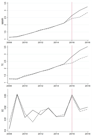
Figure 1.
NMWPI, TC, EC time series for Hebei (solid) and synthetic Hebei (gotted).
According to Figure 1, before the levy of the water resources tax, Hebei’s NMWPI and TC have maintained an upward trend, and both the treated outcome and its counterfactual follow a positive trend. The EC fluctuates, but the amplitude is not large (the difference between the maximum value and the minimum value is about 0.03). After the implementation of the WRTR policy, the real Hebei’s NMWPI and TC have risen faster and have been higher than the synthetic Hebei’s NMWPI and TC. The gap between the two has gradually widened over time. The EC of real Hebei is smaller than that of synthetic Hebei. Specifically, from 2008 to 2015, the average gap in the NMWPI between real Hebei and synthetic Hebei was −0.025. Since the implementation of the policy in 2016, the gap in the NMWPI between real Hebei and synthetic Hebei began to be positive, which was 0.40, 0.54, and 0.74 higher than that of synthetic Hebei, and the ATT, computed as the average post-treatment percent gap, amounts to 18.0%. We know the WRTR has a significant role in promoting the NMWPI in Hebei Province in the short term. For TC, similar to the change in the NMWPI over time, the average gap of TC between real Hebei and synthetic Hebei is 0.006 in pre-treatment period, and the ATT, amounts to 17.3%. The WRTR also significantly promote TC of Hebei in the short term. For RW, we observe a very small magnitude of gap, the ATT is 0.7%, therefore, may not be such a sizable post-policy gap for the treated unit. Since the NMWPI = TC × EC, we can know that most of the changes in the NMWPI are derived from TC.
6. Robustness Test
The study found that the NMWPI and TC of real Hebei and synthetic Hebei showed large differences after the WRTR, while EC did change slightly. It is not clear whether the effect is statistically significant. This phenomenon may not be due to the reform; there may be accidents or some unobserved external factors. Therefore, in order to test the validity of the above empirical results, a placebo test and a ranking test are employed to verify the significance of the implementation effects of the WRTR policy to exclude the interference of contingency and other factors.
6.1. Placebo Test
First, this article assumes that policy intervention has no causal impact on provinces. Then, select a province from the control group as a pseudo-intervention group. This means to consider control units as treated one at a time, to estimate their respective synthetic control, and to compute the treatment effect given by the post-policy differences between control unit outcomes and their counterfactuals, the estimated policy effects of 21 provinces can be obtained, and the estimated distribution of the WRTR policy effects can be obtained. If the water performance of a province is not well fitted before the WRTR policy, the ability to explain the changes in water performance will also decrease after the policy. Therefore, we delete the poor fit provinces before the policy.
The black solid line represents the influence of the WRTR policy on the NMWPI, TC, and EC of Hebei Province, while the light solid line is the pseudo policy effect estimated by the synthetic control method as a pseudo-intervention unit in other provinces. We can detect the location of the assessed Hebei WRTR policy effect in the above distribution. If the estimated treatment effect for the actually treated unit, Hebei, is larger relative to the ones estimated for the control provinces, the significance of the estimated effects is ascertained. If the line of real Hebei is in the tail extreme position of the distribution, the null hypothesis is rejected, which shows that the WRTR has a significant impact on Hebei’s water performance. If the line is in the middle of the distribution, it means that the random sampling of a province as a treated unit can obtain a significant policy effect, that is, in fact, the provinces that are not treated by the policy also have significant effect. In this case, we could not refuse the null hypothesis, which indicates that the policy has no significant effect on the water performance.
Figure 2 shows that by 2016, the degree of change in the NMWPI, TC, and EC in the Hebei is in the middle of the distribution. However, after the implementation of the WRTR in 2016, the gap in the NMWPI and TC has gradually become larger, which is located outside other provinces and at the extreme end of all paths. For the NMWPI and TC, the average treated effect (ATT) estimates of the province (Hebei) actually affected by policy are the largest, exceeding the other placebo ATT estimates. However, this does not hold for EC. Therefore, the placebo test shows that the WRTR policy has a statistically significant impact on NMWPI and TC, but no impact on EC.
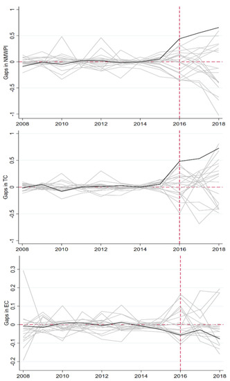
Figure 2.
Placebo tests: Hebei (black line) and control units (grey lines).
Another form of the placebo test is to calculate the distribution of the ratio of “Post period-MSPE” to “Pre period-MSPE” [11,35]. The basic logic is that, if the WRTR policy is effective, the synthetic control method will not be able to predict the real post-treated NMWPI, TC, and EC of Hebei province, resulting in a larger Post-period MSPE. However, before the policy is implemented, if synthetic Hebei cannot predict the outcome variable of real Hebei well (larger MSPE before intervention), which will also lead to a lager MSPE after intervention, then the ratio of the two can be used to control the disturbance of the former. Therefore, the significance of the treatment effect can be well recognized by the ratio of Post-period MSPE/Pre-period-MSPE. That is, if the WRTR policy in Hebei does have a larger effect, the placebo effect of other provinces is relatively lower; in Figure 3, we can observe that the Post-period MSPE/Pre-period-MSPE of Hebei province is higher than that of the other provinces.
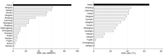
Figure 3.
MSE ratio for Hebei (black) and control units (white).
The mean square error ratio test shows that the NMWPI of Hebei and the mean square error ratio of the TC are both the maximum values of 90 and 75, respectively. Therefore, the policy effect is significant for both. Through the analysis above, the WRTR policy has statistical significant effect for the NMWPI and TC, but no significant effect on EC. As the goal of this policy, water performance has improved. Through ML decomposition, we can know that the increase in the total factor productivity of water resources seems to come from technological progress (TC) rather than technological efficiency (EC). This may result from the policy objective of the WRTR policy being to raise the tax standards for the high water consumption by industry and excess use areas where groundwater is over-exploited but to maintain necessary production and domestic water. As the cost of water increases, firms have to improve their technical level, such as buying more advanced equipment and reusing more wastewater so TC has a big rise. Because Hebei Province is more heavy industry, in the case of rapid economic development in China, there is a certain demand for heavy industrial products. In addition, special industries, such as car washing and golf courses, belong to the service industry, and they are becoming an indispensable part of life. These reasons may lead to the unchanged EC.
6.2. DID Approach
Finally, we employ the conventional policy evaluation method, DID, to estimate the policy effect. The treated unit is only one province in Hebei, the treated variable Hebei is 1. In other provinces, the time variable is set to 0 before 2016, 1 after 2016, and the DID terms are treat and time interactions, indicating the effect of the policy implementation. Table 7 reports the results estimated using the DID method; as you can see, the WRTR policy has achieved statistically significant results, the NMWPI is approximately increased by 63.9%, the TC increased 83.0 percent, and similar to the synthetic control estimates, the change in EC is not statistically significant and other control variables are the same with the synthetic control method. Since there is likely to be collinearity among these control variables, for example GDP per capita, education, and share of industry, we do not pay much attention to the significance of these variables as their coefficient is biased. The DID estimator obtained is unbiased only under the condition that the outcome variables of the treated group and the control group before the policy shock are not significantly different, that is, the parallel trend assumption (PTA) should be satisfied. If the PTA is violated, the prediction is biased. We prove this by conducting parallel trend tests on the NMWPI and TC. Figure 4 plots the estimated treatment effects and their respective confidence intervals for each year. For the NMWPI, the treatment effect in 2017 and 2018 was significant at the 10% level, and it was not significant before 2017. For TC, the treatment effects in 2017 and 2018 are both significant at the 10% level. The parallel trend shows that the policy will only have a significant effect in 2017 and 2018. Specifically, though the PTA holds, other unobserved determinants or special events would have different impacts over time. In 2016, China implemented several water resources policies, such as “the implementation of clean production technology in key industries for water pollution prevention and control” and new “Water Pollution Prevention and Control Law of the People’s Republic of China”, and China appointed local government heads as river chiefs across the nation to clean up and protect water resources (River Chief System). As a pilot province of water resources tax, Hebei is likely to be more sensitive to water resources tax, so the response of the treatment group (Hebei province) and the control group may be different. Especially if the reaction of the treatment group is larger than the control group, DID will be overestimated. Since Hebei is one of the most water-deficient provinces in China, its response to water policies are likely to exceed most provinces. Therefore, controlling for this variation is at the heart of this paper’s motivation to employ the SCM.
Table 7.
DID regression estimates (2008–2018) for NMWPI, TC, and EC.
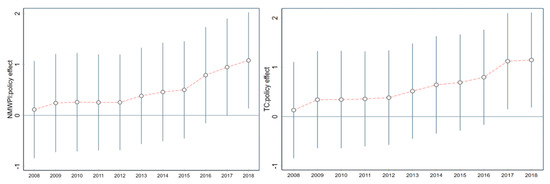
Figure 4.
Pre-and post-treatment policy effects (left: MNWPI, right: TC).
7. Conclusions
This article uses the case of water tax reform in Hebei, China, to investigate the policy effect on water resource performance. For the first time, the impact of water tax reform on water resource utilization is analyzed, and the research results verified the effect of the policy. First, this paper considers the water efficiency under environmental constraints by using the the NDDF-ML index method, which allows undesirable outputs and desirable outputs to decrease and expand in different proportions, to measure the water performance (NMWPI) of each province in China from 2008 to 2018, and decomposes it into technical changes (TC) and technical efficiency (EC). Secondly, there are problems in how to select the control group and how to make statistical inferences in the case study. The synthetic control method that we adopted was to assign appropriate weights to the control group by mining the information of the data to obtain a control group that fits the best before the event occurs. Then, the “counterfactual” phenomenon constructed by the synthetic control method and the real water resources utilization performance of Hebei Province (NMWPI), Technical changes (TC), and technical efficiency (EC) were compared. Research shows that China’s total factor productivity of water resources has been rising in the past 10 years, and the WRTR policy in Hebei has further promoted the increase of the NMWPI and TC, but the EC has remained unchanged in the whole period. After the placebo test and the ranking test, our results are still stable. The DID method proves that since the implementation of multiple water resources policies in 2016 has different effects on different provinces, the DID method overestimates the effects of water resource tax policies. Therefore, it is reasonable to use the synthetic control method. The findings contribute to the further promotion of the policy on water resources tax reform, as it has achieved positive results. Our evidence shows that taxes on resources can help to improve the efficiency of resource utilization, and increasing the cost of resources can reduce the negative externalities to a certain extent. The possible reason for this is that increasing the cost of water can promote enterprises, especially those with high water consumption and high pollution, to adopt advanced production equipment and increase the reuse of water resources. In addition, the revenue from the resource tax can used to subsidize enterprises to use more advanced and resource-saving technologies to carry out ecological projects of water resources protection. However, the decomposition of the water performance index shows that the improvement in water performance comes from technological progress, not the improvement of efficiency. The change in technical efficiency is very small, and the allocation of water resources is still an urgent problem. The government needs more effective measures, such as forcing the closure of high water consumption and high pollution enterprises or guiding these enterprises to move to places rich in water resources for production. In the case of the shortage of water resources, we can also establish a water rights trading market to make water resources reallocate to more environmentally friendly sectors. China is the country with the highest population in the world and is also one of the most water-scarce countries in the world. Water resources are ultimately important to people’s lives and production, especially in developing countries where resource utilization efficiency is lower. Fortunately, some countries, such as China, have begun to experiment with policies to improve the performance of water resources.
8. Disscussion
The findings contribute to the further promotion of the policy on water resources tax reform, as it has achieved positive results. Our evidence shows that a tax on resources can help to improve the efficiency of resource utilization and increasing the cost of resource can reduce the negative externalities to a certain extent. However, due to the limitation of data, our research did not specifically explore the reasons for the improvement of water resources efficiency, technological change, and efficiency change. The possible reason for this is that increasing the cost of water can promote enterprises, especially those with high water consumption and high pollution, to adopt advanced production equipment and increase the reuse of water resources. In addition, the revenue from the resource tax can used to subsidize enterprises to use more advanced and resource-saving technologies to carry out ecological projects of water resources protection. The decomposition of the water performance index shows that the improvement in water performance comes from technological progress, not the improvement of efficiency. The change in technical efficiency is very small, and the allocation of water resources is still an urgent problem. The government needs more effective measures, such as forcing the closure of high water consumption and high pollution enterprises or guiding these enterprises to move to places rich in water resources for production. The micro-mechanism of the impact of a water resources tax remains to be further studied. China is the country with the highest population in the world, and it is also one of the most water-scarce countries in the world. Water resources are ultimately important to people’s lives and production, especially in developing countries where resource utilization efficiency is lower. Fortunately, some countries, such as China, have begun to experiment with policies to improve the performance of water resources.
Author Contributions
L.H. is a full professor of economics. K.C. is a PHD candidate supervised by L.H. Both authors contributed significantly in the project. L.H. acquired all the funding supports. K.C. calculated the results under L.H.’s supervision. L.H. and K.C. analyzed the data, discussed the results, and co-wrote the manuscript. All authors have read and agreed to the published version of the manuscript.
Funding
This work was supported by the State Key Project of the National Social Science Foundation of China (Grant No. 19AZD003).
Institutional Review Board Statement
Not applicable.
Informed Consent Statement
Not applicable.
Data Availability Statement
The data are from the China Statistical Yearbook of the National Bureau of statistics of China, at http://www.stats.gov.cn/ (accessed on 30 October 2021) and some missing data are collected manually from the websites of provincial governments.
Conflicts of Interest
The authors declare no conflict of interest.
Appendix A
Table A1.
Estimation results of the technology change (TC) in China.
Table A1.
Estimation results of the technology change (TC) in China.
| Province | 2008 | 2009 | 2010 | 2011 | 2012 | 2013 | 2014 | 2015 | 2016 | 2017 | 2018 |
|---|---|---|---|---|---|---|---|---|---|---|---|
| Shanghai | 1.302 | 1.343 | 1.562 | 1.641 | 1.802 | 1.868 | 2.055 | 2.346 | 2.929 | 3.073 | 3.768 |
| Yunnan | 1.211 | 1.045 | 1.179 | 1.262 | 1.301 | 1.321 | 1.616 | 1.921 | 1.902 | 1.945 | 2.186 |
| Jilin | 1.215 | 1.107 | 1.176 | 1.245 | 1.403 | 1.386 | 1.535 | 1.707 | 1.740 | 2.087 | 2.227 |
| Ningxia | 1.125 | 1.089 | 1.119 | 1.146 | 1.193 | 1.211 | 1.242 | 1.264 | 1.315 | 1.189 | 1.150 |
| Anhui | 1.260 | 1.150 | 1.569 | 1.426 | 1.721 | 1.915 | 2.196 | 2.399 | 2.421 | 3.096 | 3.106 |
| Guangdong | 1.432 | 1.405 | 1.826 | 2.187 | 2.340 | 2.526 | 2.800 | 2.925 | 3.145 | 3.129 | 3.687 |
| Guangxi | 1.220 | 0.912 | 1.079 | 1.272 | 1.377 | 1.672 | 1.876 | 2.094 | 1.979 | 2.779 | 3.195 |
| Xinjiang | 1.010 | 0.956 | 1.056 | 1.208 | 1.267 | 1.168 | 1.230 | 1.292 | 1.422 | 1.582 | 1.676 |
| Jiangsu | 1.255 | 1.279 | 1.474 | 1.605 | 1.867 | 2.141 | 2.414 | 2.703 | 2.991 | 3.074 | 3.564 |
| Jiangxi | 1.181 | 1.041 | 1.219 | 1.347 | 1.551 | 1.635 | 1.849 | 2.107 | 2.148 | 2.517 | 2.827 |
| Hebei | 1.247 | 1.270 | 1.435 | 1.591 | 1.773 | 1.927 | 2.119 | 2.316 | 2.834 | 3.266 | 3.534 |
| Zhejiang | 1.266 | 1.267 | 1.472 | 1.421 | 1.561 | 1.701 | 1.862 | 2.046 | 2.364 | 2.850 | 3.126 |
| Hainan | 1.020 | 0.827 | 0.897 | 0.829 | 0.834 | 0.864 | 0.799 | 0.783 | 1.292 | 1.370 | 1.077 |
| Hubei | 1.141 | 1.019 | 1.286 | 1.503 | 1.782 | 1.850 | 2.043 | 2.192 | 2.443 | 2.894 | 3.167 |
| Hunan | 1.167 | 0.956 | 1.081 | 1.355 | 1.662 | 1.839 | 2.010 | 2.189 | 2.698 | 2.848 | 2.710 |
| Fujian | 1.231 | 1.075 | 1.506 | 1.592 | 1.791 | 1.827 | 2.041 | 2.246 | 2.477 | 2.788 | 3.051 |
| Guizhou | 1.099 | 0.910 | 1.023 | 1.117 | 1.111 | 1.009 | 1.038 | 1.197 | 1.583 | 1.737 | 2.213 |
| Liaoning | 1.013 | 1.002 | 1.128 | 1.243 | 1.386 | 1.481 | 1.634 | 1.777 | 1.549 | 1.631 | 1.476 |
| Chongqing | 1.248 | 1.044 | 1.059 | 1.244 | 1.541 | 1.735 | 1.998 | 2.255 | 2.510 | 2.608 | 2.883 |
| Qinghai | 1.072 | 1.162 | 1.160 | 1.205 | 1.266 | 1.295 | 1.334 | 1.353 | 1.413 | 1.991 | 1.453 |
| Heilongjiang | 1.252 | 0.993 | 1.172 | 1.360 | 1.752 | 1.709 | 1.792 | 1.899 | 2.249 | 2.450 | 2.525 |
Table A2.
Estimation results of the efficiency change (EC) in China.
Table A2.
Estimation results of the efficiency change (EC) in China.
| Province | 2008 | 2009 | 2010 | 2011 | 2012 | 2013 | 2014 | 2015 | 2016 | 2017 | 2018 |
|---|---|---|---|---|---|---|---|---|---|---|---|
| Shanghai | 1.032 | 1.175 | 1.092 | 1.162 | 1.130 | 1.172 | 1.128 | 1.104 | 1.050 | 1.184 | 1.035 |
| Yunnan | 0.895 | 0.916 | 0.914 | 0.914 | 0.930 | 0.934 | 1.047 | 1.058 | 1.142 | 1.166 | 1.237 |
| Jilin | 0.907 | 0.898 | 0.895 | 0.894 | 0.896 | 0.911 | 0.896 | 0.895 | 0.921 | 0.900 | 0.902 |
| Ningxia | 1.120 | 1.161 | 1.142 | 1.104 | 1.086 | 1.098 | 1.084 | 1.087 | 1.067 | 1.350 | 1.166 |
| Anhui | 0.935 | 0.901 | 1.081 | 0.936 | 1.080 | 1.028 | 1.040 | 1.021 | 1.146 | 0.974 | 1.003 |
| Guangdong | 0.988 | 1.200 | 1.068 | 1.095 | 1.115 | 1.115 | 1.124 | 1.124 | 1.130 | 1.200 | 1.068 |
| Guangxi | 0.894 | 0.978 | 0.933 | 0.967 | 0.985 | 1.081 | 1.035 | 1.035 | 1.162 | 0.963 | 1.060 |
| Xinjiang | 1.200 | 0.971 | 0.898 | 0.901 | 0.896 | 0.902 | 0.895 | 0.896 | 0.904 | 0.898 | 0.892 |
| Jiangsu | 1.038 | 1.169 | 1.097 | 1.136 | 1.092 | 1.101 | 1.112 | 1.117 | 1.125 | 1.200 | 1.067 |
| Jiangxi | 0.900 | 0.894 | 1.007 | 0.979 | 1.043 | 0.980 | 1.006 | 1.006 | 0.991 | 0.960 | 0.983 |
| Hebei | 0.902 | 0.931 | 0.911 | 0.918 | 0.914 | 0.920 | 0.912 | 0.912 | 0.931 | 0.918 | 0.920 |
| Zhejiang | 0.991 | 1.133 | 1.049 | 1.229 | 1.130 | 1.135 | 1.132 | 1.129 | 1.009 | 1.090 | 1.099 |
| Hainan | 1.192 | 1.375 | 1.079 | 1.229 | 1.137 | 1.078 | 1.194 | 1.174 | 0.917 | 1.116 | 1.348 |
| Hubei | 0.912 | 0.934 | 0.917 | 0.916 | 0.932 | 0.896 | 0.900 | 0.896 | 0.912 | 0.895 | 0.893 |
| Hunan | 0.910 | 0.980 | 0.895 | 0.926 | 0.941 | 0.914 | 0.908 | 0.905 | 0.924 | 0.895 | 0.916 |
| Fujian | 0.909 | 1.004 | 0.910 | 0.896 | 0.894 | 0.914 | 0.900 | 0.901 | 0.897 | 0.921 | 0.895 |
| Guizhou | 0.925 | 1.030 | 0.896 | 0.902 | 0.906 | 0.897 | 0.939 | 1.009 | 1.147 | 1.039 | 1.208 |
| Liaoning | 0.913 | 0.989 | 0.956 | 0.977 | 0.971 | 0.996 | 0.968 | 0.965 | 1.119 | 1.057 | 1.134 |
| Chongqing | 0.897 | 0.918 | 0.895 | 0.911 | 0.924 | 0.901 | 0.901 | 0.897 | 0.895 | 0.898 | 0.885 |
| Qinghai | 1.154 | 1.139 | 1.201 | 1.170 | 1.162 | 1.182 | 1.176 | 1.189 | 1.166 | 0.970 | 1.572 |
| Heilongjiang | 0.907 | 1.045 | 0.898 | 0.904 | 0.989 | 0.900 | 0.898 | 0.896 | 0.922 | 0.902 | 0.888 |
References
- Mcdonald, R.I.; Weber, K.; Padowski, J.M.; Schneider, C.; Green, P.A. Water on an urban planet: Urbanization and the reach of urban water infrastructure. J. Abbr. 2014, 27, 96–105. [Google Scholar] [CrossRef] [Green Version]
- Srinivasan, V.; Konar, M.; Sivapalan, M. A dynamic framework for water security. Water Secur. 2017, 1, 12–20. [Google Scholar] [CrossRef]
- Muller, M. Lessons from Cape Town’s drought. Nature 2018, 559, 174–176. [Google Scholar] [CrossRef] [Green Version]
- Chen, Z.; Kahn, M.E.; Liu, Y.; Wang, Z. The consequences of spatially differentiated water pollution regulation in China. J. Environ. Econ. Manag. 2018, 15, 159–177. [Google Scholar] [CrossRef]
- Tao, T.; Xin, K. A sustainable plan for China’s drinking water: Tackling pollution and using different grades of water for different tasks is more efficient than making all water potable. Nature 2014, 551, 527–529. [Google Scholar] [CrossRef] [PubMed]
- Ercin, A.E.; Hoekstra, A.Y. Water footprint scenarios for 2050: A global analysis. Eur. J. Oper. Res. 2014, 64, 71–82. [Google Scholar] [CrossRef] [PubMed]
- Wang, J.; Wei, Y.D. Agglomeration, environmental policies and surface water quality in China: A study based on a quasi-natural experiment. Sustainability 2019, 11, 5394. [Google Scholar] [CrossRef] [Green Version]
- Charnes, A.; Cooper, W.W.; Rhodes, E. Measuring the efficiency of decision making units. Environ. Int. 1978, 2, 42–444. [Google Scholar] [CrossRef]
- Färe, R.; Grosskopf, S.; Norris, M.; Zhang, Z. Productivity growth, technical progress, and efficiency change in industrialized countries. Americian Econ. Rev. 1994, 84, 66–83. [Google Scholar]
- Abadie, A.; Gardeazabal, J. The economic costs of conflict: A case study of the Basque country. Americian Econ. Rev. 1994, 93, 113–132. [Google Scholar] [CrossRef] [Green Version]
- Abadie, A.; Diamond, A.; Hainmueller, J. Synthetic Control Methods for Comparative Case Studies: Estimating the Effect of California’s Tobacco Control Program. J. Am. Stat. Assoc. 2010, 105, 493–505. [Google Scholar] [CrossRef] [Green Version]
- Mushtaq, S.; Khan, S.; Da We, D.; Hanjra, M.A.; Hafeez, M.; Asghar, M.N. Evaluating the impact of Tax-for-Fee reform (Fei Gai Shui) on water resources and agriculture production in the Zhanghe Irrigation System, China. Food Policy 2008, 33, 576–586. [Google Scholar] [CrossRef] [Green Version]
- Yep, R. Can “Tax-for-Fee” reform reduce rural tension in China? The process, progress and limitations. China Q. 2004, 177, 42–70. [Google Scholar] [CrossRef]
- Hui, Q. Tax and Fee Reform, village autonomy, and central and local finance. Chin. Econ. 2004, 38, 3–35. [Google Scholar]
- Mushtaq, S.; Dawe, D.; Hong, L.; Moya, P. An assessment of the role of ponds in the adoption of water-saving irrigation practices in the Zhanghe irrigation system, China. Agric. Water Manag. 2006, 83, 100–110. [Google Scholar] [CrossRef]
- Heerink, N.; Qu, F.; Kuiper, M.; Shi, X.; Tan, S. Policy reforms, rice production and sustainable land use in China: A macro-micro analysis. Agric. Syst. 2007, 94, 784–800. [Google Scholar] [CrossRef]
- Luo, R.; Zhang, L.; Huang, J.; Rozelle, S. Elections, fiscal reform and public goods provision in rural China. J. Comp. Econ. 2007, 35, 583–611. [Google Scholar] [CrossRef]
- Chen, Z.R.; Nie, P.Y. Analysis of the Fee-to-Tax Reform on Water Resources in China. Front. Energy Res. 2021, 9, 752592. [Google Scholar] [CrossRef]
- Ma, Z.; Zhao, J.; Ni, J. Green Tax Legislation for Sustainable Development in China. Singap. Econ. Rev. 2018, 63, 31–45. [Google Scholar] [CrossRef]
- Zhao, A.F.; Zhang, Y.X. Study on the impact of water resources tax on water consumption and water efficiency–quasi natural experiment based on the pilot expansion of water resources tax. Tax Res. 2021, 2, 1059–1083. [Google Scholar]
- Yang, D.Q.; Zhao, L.; Yang, D.D. Does water resource tax improve water efficiency—Empirical evidence from Hebei. Tax Res. 2020, 8, 836–842. [Google Scholar]
- Kennedy, J.J. From the tax-for-fee reform to the abolition of agricultural taxes: The impact on township governments in north-west China. China Q. 2007, 189, 43–59. [Google Scholar] [CrossRef]
- Chen, S.; Golley, J. ‘Green’ productivity growth in China’s industrial economy. Energy Econ. 2014, 44, 89–98. [Google Scholar] [CrossRef]
- Zhang, N.; Choi, Y. A note on the evolution of directional distance function and its development in energy and environmental studies 1997–2013. Renew. Sustain. Energy Rev. 2014, 33, 50–59. [Google Scholar] [CrossRef]
- Chung, Y.; Färe, R.; Grosskopf, S. Productivity and Undesirable Outputs: A Directional Distance Function Approach. J. Environ. Manag. 1997, 51, 229–240. [Google Scholar] [CrossRef] [Green Version]
- Du, K.; Huang, L.; Yu, K. Sources of the potential CO2 emissions reduction in China: A nonparametric metafrontier approach. Appl. Energy 2014, 115, 491–501. [Google Scholar] [CrossRef]
- Zhou, P.; Ang, B.W.; Wang, H. Energy and CO2 emission performance in electricity generation: A non-radial directional distance function approach. Eur. J. Oper. Res. 2012, 221, 625–635. [Google Scholar] [CrossRef]
- Fukuyama, H.; Weber, W.L. A directional slacks-based measure of technical inefficiency. Socio-Econ. Plan. Sci. 2010, 43, 274–287. [Google Scholar] [CrossRef]
- Färe, R.; Grosskopf, S.; Lovell, C.A.K.; Pasurka, C. Multilateral productivity comparisons when some outputs are undesirable: A nonparametric approach. Rev. Econ. Stat. 1989, 71, 90–98. [Google Scholar] [CrossRef]
- Zhang, N.; Choi, Y. Environmental energy efficiency of China’s regional economies: A non-oriented slacks-based measure analysis. Soc. Sci. J. 2013, 50, 225–234. [Google Scholar] [CrossRef]
- Caves, D.W.; Christensen, L.R.; Diewert, W.E. Multilateral Comparisons of Output, Input, and Productivity Using Superlative Index Numbers. Econ. J. 1982, 92, 73–86. [Google Scholar] [CrossRef]
- Xiong, Y.J.; Hao, X.R.; Liao, C.; Zeng, Z.N. Relationship between water-conservation behavior and water education in Guangzhou, China. Environ. Earth Sci. 2016, 75, 1–9. [Google Scholar] [CrossRef]
- Zhao, L.; Sun, C.; Liu, F. Interprovincial two-stage water resource utilization efficiency under environmental constraint and spatial spillover effects in China. J. Clean. Prod. 2017, 164, 715–725. [Google Scholar] [CrossRef]
- Qian, Y.; Liu, H. Regional Disparity and Influencing Factors of Agricultural Water Resources Efficiency with the Constraint of Pollution. J. Quant. Tech. Econ. 2015, 1, 114–158. [Google Scholar]
- Bueno, M.; Valente, M. The effects of pricing waste generation: A synthetic control approach. J. Environ. Econ. Manag. 2019, 96, 274–285. [Google Scholar] [CrossRef] [Green Version]
Publisher’s Note: MDPI stays neutral with regard to jurisdictional claims in published maps and institutional affiliations. |
© 2021 by the authors. Licensee MDPI, Basel, Switzerland. This article is an open access article distributed under the terms and conditions of the Creative Commons Attribution (CC BY) license (https://creativecommons.org/licenses/by/4.0/).