A Novel Machine Learning-Based Price Forecasting for Energy Management Systems

Abstract

Price forecasting (PF) is the primary concern in distributed power generation. This paper presents a novel and improved technique to forecast electricity prices. The data of various power producers, Capacity Purchase Price (CPP), Power Purchase Price (PPP), Tariff rates, and load demand from National Electric Power Regulatory Authority (NEPRA) are considered for MAPE reduction in PF. Eight time-series and auto-regression algorithms are developed for data fetching and setting the objective function. The feed-forward ANFIS based on the ML approach and space vector regression (SVR) is introduced to PF by taking the input from time series and auto-regression (AR) algorithms. Best-feature selection is conducted by adopting the Binary Genetic Algorithm (BGA)-Principal Component Analysis (PCA) approach that ultimately minimizes the complexity and computational time of the model. The proposed integration strategy computes the mean absolute percentage error (MAPE), and the overall improvement percentage is 9.24%, which is valuable in price forecasting of the energy management system (EMS). In the end, EMS based on the Firefly algorithm (FA) has been presented, and by implementing FA, the cost of electricity has been reduced by 21%, 19%, and 20% for building 1, 2, and 3, respectively.

1. Introduction

It is necessary to forecast electricity prices for the Independent System Operator (ISO) and the end-users and marketers. Generally, the profit bidders in the potential electricity market need the future electricity prices in order to earn a good profit; however, the existing electricity market has made PF more complex as it is highly deregulated and non-linear. Due to the system’s non-linear and unstable behavior, accurate prediction of prices has become more complex. It also affects the bidding policies in the electricity market. The PF techniques are categorized into three classes according to their specific forecasting models: The statistical model, time-series model, and AI-based models [1]. The AI-based forecasting approach has attracted much attention in recent years. It assures a guaranteed level of accuracy of price estimation compared to unstable variations of dependent or independent variables in the statistical model.

The current energy market depends on renewable energy resources because these are playing a leading role in fulfilling the energy demand. In the rising energy demand, an economical solution is needed to address persistent issues [2]. An exhaustive work concludes that renewable energy generation resources have an extensive impact on energy unit prices. The generation-side and demand-side companies are in contact to develop a steadiness between supply and demand. An optimized home energy management system (EMS) proposed in [3] computes the unit price of electricity by utilizing an RES and battery storage system. The energy unit price is determined by correspondence from generation groups with the requirement from the load-allocation bodies. The subsequent energy demand is calculated from load allocation bodies and fed to the supply side to avoid inconveniences such as an electricity shutdown.

On the other hand, the dependability and protection of the electricity system are managed by a regulatory authority to harmonize with local distribution companies. This regulatory authority also determines the energy unit price [4]. The cost-effective solution in any domain is a considerable factor. Recently, the energy unit PF has been presented, and diverse performances have also been suggested. Numerous areas, including signal processing, statistical modeling, Machine Learning (ML), big-data analysis, and Artificial Intelligence (AI), are anticipated tools [5]. An overview of the latest trends in power systems is presented in Figure 1.

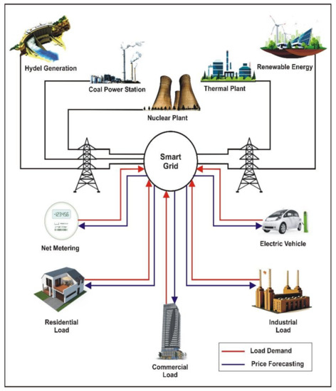
Figure 1. Overview of latest trends in power system.

Several methods have been proposed to forecast load consumption and per-unit prices, such as engineering and statistical methods. Many researchers are working on AI applications such as the Artificial Neural Network (ANN), Support Vector Machine (SVM), evolutionary programming, expert system, fuzzy logic (FL), and LF-related problems. In this regard, many hybrid AI models have been developed to monitor and schedule. They forecast electric load, including neural networks, fuzzy expert systems, fuzzy neural networks (FNN), neural expert systems, neural-GA, and fuzzy expert [6,7,8,9,10].

Various steps and efforts are proposed in the latest research to meet the large gap between demands and supply. On the other hand, an approach to decision-making and medical diagnosis problems using the concept of spherical fuzzy sets is also evaluated in [11]. Moreover, electricity cannot be stored in large amounts. The construction of newer power plants is not an ultimate solution as it may lead to carbon emissions and the depletion of resources [12]. Electric utilities have realized that consumer demands cannot be met satisfactorily by adding new generating capacity alone [13]. Demand-Side Management (DSM) and Demand Response (DR) are the terms used for energy management. These deal with actions that influence consumers’ energy usage patterns in peak load times [14]. It also includes decision making, implementation, and the following of activities of utilities to motivate the consumers to modify their level and pattern of electricity consumption according to the retail price [15]. Hence, the present focus of researchers is in the domain of energy management.

This article considers the data of various power producers, CPPs, PPPs, Tariff rates, and load demand from NEPRA for MAPE reduction in PF. Eight time-series and auto-regression algorithms are developed for data fetching and setting the objective function as shown in Figure 2. The feed-forward ANFIS is based on the ML approach to forecast the PF by taking the inputs from time series and auto-regression algorithms. Best-feature selection is conducted by adopting the BGA-PCA approach. It reduces the repeated, irrelevant, and unnecessary data and ultimately minimizes the model’s complexity and computational time. The proposed integration strategy computes the MAPE according to the steps mentioned above and obtains significant improvements.

The contributions of this paper are well accomplished and summarized.

• NEPRA, Pakistan data are considered where the PF is optimized by reducing the MAPE.
• Eight time-series and autoregression algorithms are developed to fetch the dataset and set the objective function, while the proposed equations set the basis for further validation as improved results validate it.
• However, feedforward ANFIS based on the ML approach is proposed. Best-feature selection is evaluated through the BGA-PCA approach.
• Our results for the PF compute the MAPE of one year by the proposed integration strategy, and the overall improvement in MAPE is 9.24%.
• In the end, EMS based on the Firefly algorithm (FA) has been implemented, and the cost of electricity has been reduced by 21%, 19%, and 20% for building 1, 2, and 3, respectively, which is valuable in price forecasting of the energy management system (EMS).

2. Related Work

The forecasting medium supports establishing system models, behavior, and plans by reviewing current and past market trends. PF is the main factor of this medium, demonstrating generation capabilities, resource handling, capital cost, profit analysis, and other system plans [16]. Load estimation and price prognoses are significant factors for prime maneuver development in these viable power energy souks. Diverse methodologies exist for price and load estimation, but without feature selection, skill methodologies are inadequate. The mentioned feature selection skill deals with the modeling of intermingling structures and nonlinearities of forecast progressions. By considering technicalities and generation site plans, electricity price estimation is a more valuable chore. The energy rate is estimated with an optimistic approach based on market-side demand and predictive forecasting. Renewable energy backs the economical energy unit price. Detailed scrutiny of market data in an arithmetical manner is a fundamental requirement in this approach [17].

Many researchers forecasted the price of electricity using the ANN strategy in traditional ways. In this regard, a multi-layer feed-forward Neural Network (MFFNN), Neuro-Fuzzy, Fuzzy Neural Network, and Adaptive Wavelet Neural Network approaches based on the different analyses were used to extract selection features of price and load signals for each hour [18,19]. The electricity price varies due to dynamic variations in load demand throughout the day; therefore, this strategy minimizes the MAPE in load and price at hourly, daily, and weekly intervals [20]. With the dynamic variations in load containing high-frequency features, error is considerably increased; therefore, this research recommends Wavelet Transform to resolve this issue.

In [21], the authors used a methodology based on feature selection with mathematical and statistical modeling, utilizing the minimum block set from the input and applying a computational filtering strategy to formulate optimized PF. The research illustrated in [22] describes a trained RNN algorithm based on the Kalman Filter (KF) to forecast the load and price of electricity using one-step and nth step prediction. The proposed study practiced informative data of the European Power System (EPS) to validate the execution of the scheme. Using the time-series-based multilayer ANN-KF model increases the forecasting speed and tracking behavior, but the implementation of KF in the ANN algorithm is relatively rigid in comparison to traditional strategies.

In previous research, the AI technique has been implemented for the long-term load and PF of electricity conventionally. In [23,24,25,26], a short-term load and PF using an NN fitting tool were used to compute hourly and daily data of weather temperature and electricity load as input features. Furthermore, the generalized-RNN indicates temperature statistics and price signals as input parameters. Both techniques accurately estimate prescribed variables, but the integration of the Radial Basic Function-Neural Network (RBF-NN) and GRNN have mutual effects that declare certain computational errors. A comparative analysis of different AI approaches is compiled in Table 1, including their limitations.

Table 1. A comparison of related work of price forecasting.

Work	Key Contribution	AI Approach	FS	Limitations
[16]	Price and LF	MFFNN	No	The dynamic variations in load contain high-frequency features, which considerably increases error
[27]	PF	ML-based ANN	No	Due to limited feature selections, it lacks statistical data, an optimized model, and demand curves.
[21]	Load and Price Forecast	RCGA	Yes	Partial environment for feature selection to minimize the validation error occurred by wrappers
[28]	Price and LF	ANN-RNN	Yes	Nominal error rate deficiency occurs in other systems
[22]	PF	RNN-KF	No	The implementation of KF in the ANN algorithm relatively rigid than traditional strategies
[29]	PF	Bivariate Distribution Scheme	No	A negative correlation factor, the forecasted price of this distribution is less than the marginal distribution
[30,31]	Price and LF	ANN-RNN	No	The integration of RBFNN and GRNN have mutual effects which declare some sort of computational errors
Proposed Work	PF with a novel Proposed Modified Strategy	ANFIS-SVR	Novel BGA-PCA	A new variety of data input and complex auto-regression methods are not analyzed.

The authors of [5] propose a user-aware DR approach to manage residential loads. User comfort and savings are considered mainly, and user comfort is modeled as a weight factor before comfort over savings. The game is based on a modified regret-matching procedure, which has the advantage of centralized and decentralized schemes. The work can be extended with multiple energy resources in the future.

Two optimization techniques, such as the FA and harmony search algorithm, are presented in this paper. These heuristic techniques are applied to different types of appliances based on their energy consumption. Single and multiple home appliances are considered in this research. Time of Use (ToU) is used as a pricing signal in the proposed technique to calculate electrical cost [32].

In [33], a new algorithm introduces this study to solve and reduce the electricity cost problem using two metaheuristics techniques, FA and Elephant herding optimization (EHO). A scheduling process is used as an HEMC to maintain the balance between the demand and load sides. This study aims to determine the low cost by considering the maximum factors of user comfort and the average-to-peak ratio. The scheduling process and performance are evaluated by the comparative analysis of these two meta-heuristic techniques.

The primary purpose of this research is the successful implementation of FA in different areas and thus the widening scope of its potential users. Table 2 presents a comparative analysis of different methodologies related to DSM.

Table 2. Comparative analysis of work related to DSM.

Work	Key Contribution	Limitations
[34]	The techniques of scheduling residential appliances are presented in this study. This study is classified into two techniques such as meta-heuristic techniques and heuristic techniques.	With the widespread use of home appliances, residential consumers need to improve the strategies for scheduling appliances.
[3]	This paper presents DSM architecture models and algorithms based on customers behavior and smart appliances integration	Implementations need to be done
[5]	Proposes autonomous Game theory DR systems to minimize the cost of power generation.	Game theory can be an alternate to DSM
[35]	This study aims to consider the factor of maximizing user comfort, peak-to-average ratio (PAR), and the low cost by considering firefly optimization (FF).	Both algorithms performed a comparative analysis of the separately implemented version to evaluate the process of scheduling devices and improve their performance.
[36]	A swarm FA implemented except meta-heuristic algorithm for a cost-effective solution	The algorithm lacks local optimism
[33]	Two meta-heuristics techniques FA and EHO is utilized for the scheduling process in a HEMC to maintain the balance between the demand and load side	Due to the integration of two meta-heuristics techniques, but the scheduling rate is low.
[37]	A comprehensive overview of the swarm intelligence of FA is performed to express performance capabilities to encourage new researchers and developers to implement it in future works.	The implementation of FA is simple and highly efficient in solving problems.
[38]	The scheme used to calculate the electrical cost in this proposed system is CPP using a Meta-heuristic algorithm	HSA perform better than FA in terms of PAR and electricity costs
[39]	Applied on different types of appliances in single or multiple homes based on their energy consumption using FA and harmony search algorithm	ToU is used as a pricing signal in the proposed technique for the calculation of the electrical cost
[40]	The proposed strategy reduces peak load and the cost by compromising the comfort of the household consumer. Optimization is performed using a multi-objective GA	Decreases the peak load and also reduces the utility bill
[41]	This article focuses on maximizing the use of renewable energy resources using different heuristic techniques	Provide consistency in daily profit and low runs.
[42]	A concessional and maximum energy consumption schedule uses the GA to reduce and production costs and improve the efficiency factor at the utility and consumer level.	It is used over the single objective, which benefits consumers with intelligent load scheduling
[43]	The author compares the performance of the HEMC, and this controller is designed for energy consumption scheduled based on the heuristic algorithm.	The heuristic technique, such as the GA-based energy management controller, performs more efficiently than other heuristic techniques.

3. Proposed Framework for Price Forecasting

This section is based on the proposed PF techniques and framework.

3.1. Time Series and Autoregression Method

The time-series-forecasting model is proposed in [44], and nine regression algorithms are introduced for the LF. In this model, time series and auto-regression methods are taken into consideration for PF. Eight models are computed, where three are AR level-1, one is exponential smoothing, and three are AR level-II.

Level I Auto-regression Model (AR1)

Variation in price demand: Peak hour P(t−1), off-peak hour P(t−2), and special holidays or weekend P(t−3):

$${\mathrm{P}}_{\mathrm{t}}={\mathsf{\beta }}_0+{\mathsf{\beta }}_1{P}_{\mathrm{t}-1}+{\mathsf{\beta }}_2{\mathrm{P}}_{\mathrm{t}-2}+{\mathsf{\beta }}_3{\mathrm{P}}_{\mathrm{t}-3}+{\mathrm{u}}_{\mathrm{t}}$$

(1)

Level I Auto-regression Model (AR2)

AR2 is modeled by adding the month auto-regression term $M_{k,t}$ where k = 1,…,12, as there are 12 months in a year.

$${\mathrm{P}}_{\mathrm{t}}={\mathsf{\beta }}_0+{\mathsf{\beta }}_1{P}_{\mathrm{t}-1}+{\mathsf{\beta }}_2{\mathrm{P}}_{\mathrm{t}-2}+{\mathsf{\beta }}_3{\mathrm{P}}_{\mathrm{t}-3}+{\displaystyle \sum }_{\mathrm{k}=1}^{12}{\mathsf{\alpha }}_{\mathrm{k}}{M}_{k,t}+{\mathrm{u}}_{\mathrm{t}}$$

(2)

Level I Auto-regression Model (AR3)

The AR3 model has an extra auto-regression term in annual, ${\mathsf{\gamma }}_k{A}_{k,\mathrm{t}}$ and for the seasons of the year $M_{k,t}$ where k = 1,…,12.

$${\mathrm{P}}_{\mathrm{t}}={\mathsf{\beta }}_0+{\mathsf{\beta }}_1{P}_{\mathrm{t}-1}+{\mathsf{\beta }}_2{\mathrm{P}}_{\mathrm{t}-2}+{\mathsf{\beta }}_3{\mathrm{P}}_{\mathrm{t}-3}+{\mathsf{\gamma }}_k{A}_{k,\mathrm{t}}+{\displaystyle \sum }_{\mathrm{k}=1}^{12}{\mathsf{\alpha }}_{\mathrm{k}}{\overline{\mathrm{M}}}_{\mathrm{k},\mathrm{t}}+u_{\mathrm{t}}$$

(3)

Support Vector Regression (SVR)

This regression forecasts ${\mathrm{P}}_{\mathrm{t}}$ by considering the inputs ${\mathrm{P}}_{\mathrm{t}-1},{\mathrm{P}}_{\mathrm{t}-2},{\mathrm{and}\mathrm{P}}_{\mathrm{t}-3}$ for each month ${\displaystyle \sum }_{\mathrm{k}=1}^{12}{\mathsf{\alpha }}_{\mathrm{k}}{\mathrm{M}}_{\mathrm{k},\mathrm{t}}$ of the annual forecasting.

$$P_{t,SVR}=SVR\left({\mathrm{P}}_{\mathrm{t}-1},{\mathrm{P}}_{\mathrm{t}-2},{\mathrm{P}}_{\mathrm{t}-3}\right)$$

(4)

Exponential Smoothing Method

This model is used where there is no monthly pricing, where $\mathsf{\alpha }$ = smooth constant, $P_{\mathrm{t}-1}$ = previous pricing, and $F_{\mathrm{t}-1}$ = PF demand.

$$P=\mathsf{\alpha }{E}_{\mathrm{t}-1}+\left(1-\mathsf{\alpha }\right)F_{\mathrm{t}-1}+u_{\mathrm{t}}$$

(5)

Level II Auto-regression Model (AR1)

In level-II, the model is applied to the data of the same series as AR1; however, the price values and residential values from customer demand modeled in the exponential smoothing method are added.

$${\mathrm{P}}_{\mathrm{t}}^{\prime }=\mathsf{\alpha }{E}_{\mathrm{t}-1}+\left(1-\mathsf{\alpha }\right)F_{\mathrm{t}-1}+u_{\mathrm{t}}$$

(6)

$${\mathrm{P}}_{\mathrm{t}}^{″}={\mathrm{y}}_{\mathrm{t}}={\mathsf{\beta }}_0+{\mathsf{\beta }}_1{\mathrm{P}}_{\mathrm{t}-1}+{\mathsf{\beta }}_2{\mathrm{P}}_{\mathrm{t}-2}+{\mathsf{\beta }}_3{\mathrm{P}}_{\mathrm{t}-3}+{\mathrm{u}}_{\mathrm{t}}$$

(7)

$${\mathrm{P}}_{\mathrm{t}}={\mathrm{y}}_{\mathrm{t}}^{\prime }-{\mathrm{y}}_{\mathrm{t}}^{″}+{\mathrm{u}}_{\mathrm{t}}$$

(8)

Level II Auto-regression Model (AR2)

In level-II, the model is applied to the data of the same series as AR2; however, price values and residential values from customer demand modeled in the exponential smoothing method are added.

$${\mathrm{P}}_{\mathrm{t}}^{\prime }=\mathsf{\alpha }{P}_{\mathrm{t}-1}+\left(1-\mathsf{\alpha }\right)F_{\mathrm{t}-1}+u_{\mathrm{t}}$$

(9)

$${\mathrm{P}}_{\mathrm{t}}^{″}={\mathsf{\beta }}_0+{\mathsf{\beta }}_1{P}_{\mathrm{t}-1}+{\mathsf{\beta }}_2{P}_{\mathrm{t}-2}+{\mathsf{\beta }}_3{P}_{\mathrm{t}-3}+{\displaystyle \sum }_{\mathrm{k}=1}^4{\mathsf{\alpha }}_{\mathrm{k}}{\mathrm{M}}_{\mathrm{k},\mathrm{t}}+{\mathrm{u}}_{\mathrm{t}}$$

(10)

$${\mathrm{P}}_{\mathrm{t}}={\mathrm{P}}_{\mathrm{t}}^{\prime }-{\mathrm{P}}_{\mathrm{t}}^{″}+{\mathrm{u}}_{\mathrm{t}}$$

(11)

Level II Auto-regression Model (AR3)

In level II, the model is applied to the data of the same series as AR3; however, the demand values and residential values from customer demand modeled in the exponential smoothing method are added.

$$P_{\mathrm{t}}^{\prime }=\mathsf{\alpha }{E}_{\mathrm{t}-1}+\left(1-\mathsf{\alpha }\right)F_{\mathrm{t}-1}+u_{\mathrm{t}}$$

(12)

$${\mathrm{P}}_{\mathrm{t}}^{″}={\mathsf{\beta }}_0+{\mathsf{\beta }}_1{P}_{\mathrm{t}-1}+{\mathsf{\beta }}_2{\mathrm{P}}_{\mathrm{t}-2}+{\mathsf{\beta }}_3{\mathrm{P}}_{\mathrm{t}-3}+{\mathsf{\gamma }}_k{Y}_{k,\mathrm{t}}+{\displaystyle \sum }_{\mathrm{k}=1}^4{\mathsf{\alpha }}_{\mathrm{k}}{\overline{\mathrm{M}}}_{\mathrm{k},\mathrm{t}}+u_{\mathrm{t}}$$

(13)

$${\mathrm{P}}_{\mathrm{t}}={\mathrm{P}}_{\mathrm{t}}^{\prime }-{\mathrm{P}}_{\mathrm{t}}^{″}+{\mathrm{u}}_{\mathrm{t}}$$

(14)

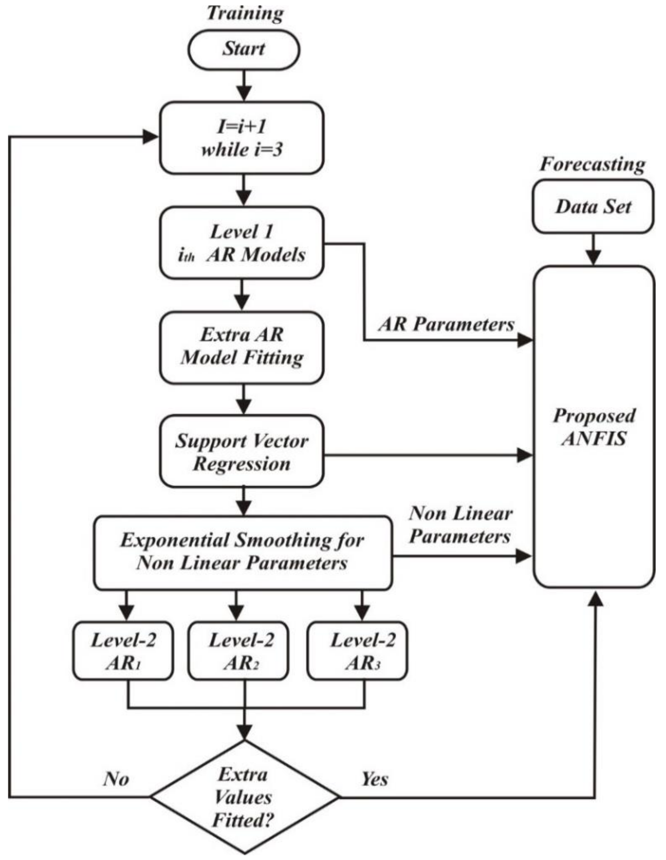
Eight time-series and autoregression algorithms in Equations (1)–(14) are developed as a training of dataset and set the objective function. The proposed equations set the basis for further validation where linear and nonlinear parameters are segregated as shown in Figure 2. However, feedforward ANFIS based on the ML approach is considered to take inputs from autoregression models and data set.

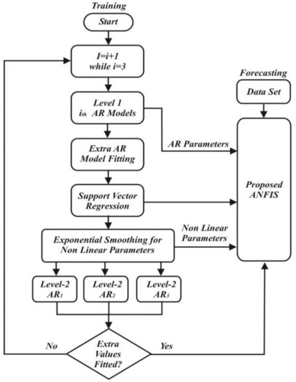
Figure 2. Illustration of input parameters of ANFIS.

3.2. Machine Learning Approach of Proposed Feedforward ANFIS

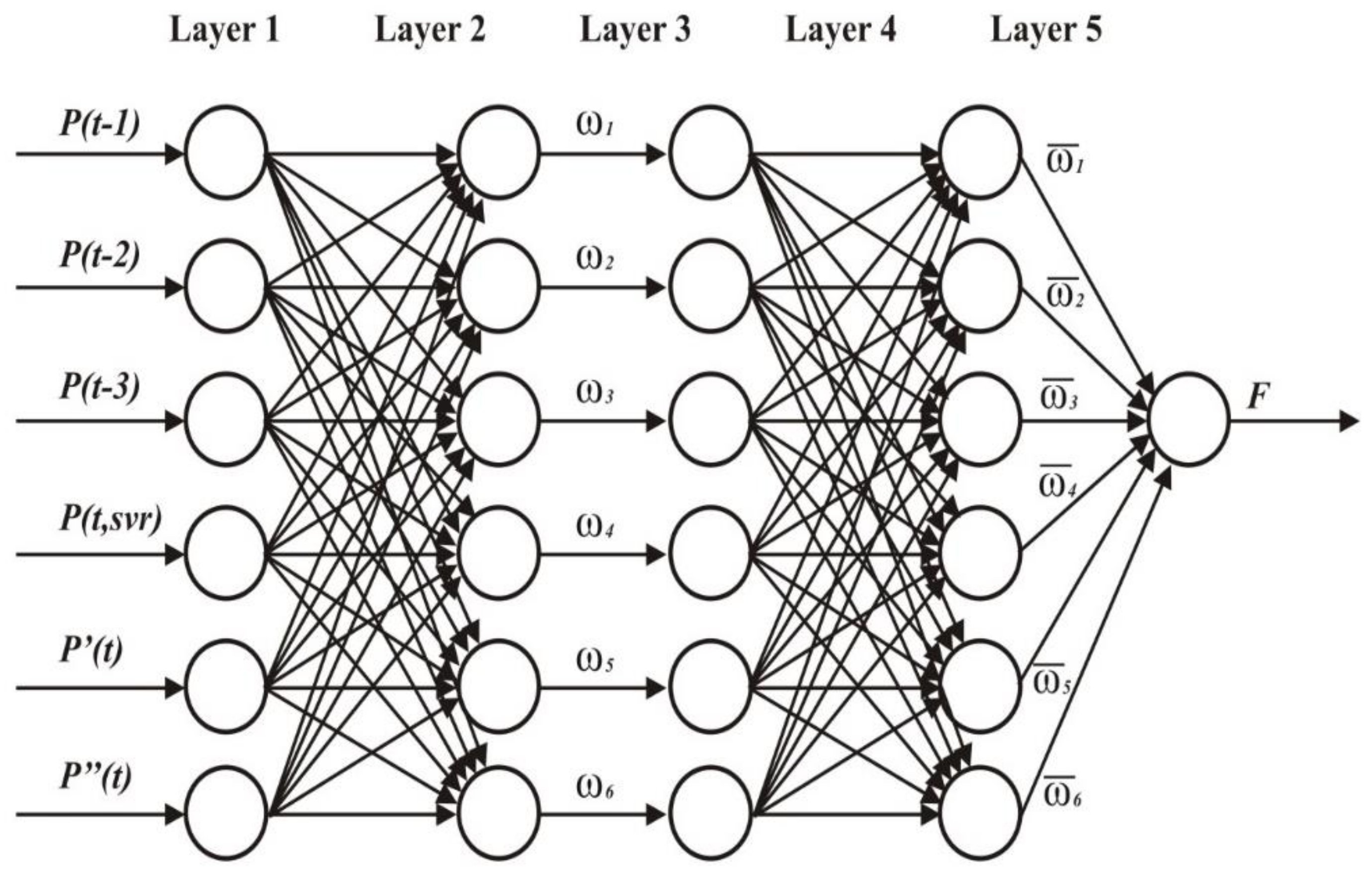
The model is further validated by the ML approach for implementing ANN, a computer model influenced by the brain and nervous system in animals or humans. The ANFIS model is presented in [45], and we modified it according to our requirement as the five stages were computed. An algorithm that uses an unmonitored training data principle to construct a load–temperature relationship is used to forecast 24 hours of load. This method uses real-time data as error-correcting function input, and simulation findings reveal that an acceptable mean absolute error percentage is better than the conventional method. In this regard, the proposed system is validated with a Feedforward Artificial Neural Network of one-year LF data. The proposed Feedforward ANFIS model consists of five stages as shown in Figure 3, where Random Forest training schemes are taken into account, and the training process is given as follows.

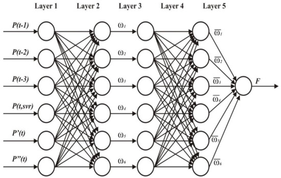
Figure 3. Flowchart for illustration of PF processes of the proposed feedback ANFIS algorithm [46].

Stage 1: In this stage, the fuzzy fiction layer simply transmits the received signal of any node to another layer. Each node for the linguistic parameter declares a member function—the output estimation of electricity price on an hourly, weekly, and monthly basis. The price estimation mainly includes power consumption statistics during the peak load time, off-peak load time, and dynamic weather conditions. The exponential methodology and level-2 AR methods are considered in Equations (15)–(18).

$$J_i^1=\mu A_i\left(P_{y-i}\right)\mathrm{for}\mathrm{i}=1,2,3$$

(15)

$$J_2^1=\mu A_2\left(P^{\prime }t\right)$$

(16)

$$J_3^1=\mu A_3\left(P^{″}t\right)$$

(17)

$$J_4^1=\mu A_4\left(P_{t,SVR}\right)$$

(18)

where $P_{y-i},P_t^{\prime },P_t^{″}\mathrm{and} P_{t,SVR}$ are the inputs to the nodes as shown in Figure 3 and $\mu A_i$ is a member function.

A is a linguistic parameter that is linked with the node function.

The μA in the model is chosen based on Equation (19):

$$\mu A_i\left(x\right)=exp{\left[-\frac{P_t-c_i}{2a_i}\right]}^2$$

(19)

where $a_i\mathrm{and}{c}_i$ are the set of premise parameters.

Stage 2: At this stage, the rule layer is employed, which simplifies the member function of PF and minimizes the burden on nodes by processing the training dataset. The node’s output expresses the firing strength of each rule and is obtained by the membership functions illustrated by Equation (20).

$$w_n=\mu A_i\left(P_{t-i}\right)\times \mu A_2\left(P^{\prime }t\right)\times \mu A_3\left(P^{″}t\right)\times \mu A_4\left(P_{t,SVR}\right) \mathrm{for}\mathrm{n}=1,2,3,4,5,6$$

(20)

Stage 3: Here, the normalization layer computes the ratio of firing strength of the relative rule to the sum of firing strengths of preceding rules. Each node at this stage is a fixed node named N. The output is given by Equation (21).

$${\overline{w}}_n=\frac{w}{w_1+w_2+w_3+w_4+w_5+w_6}$$

(21)

Stage 4: At this stage, the defuzzification layer evaluates the output for each rule by taking the product of normalized firing strength from the previous stage and the first-order Sugeno Model. The nodes at this stage are based on adaptive nodes.

$${\theta }_n^4={\overline{w}}_n{f}_{n }={\overline{w}}_n\left(k_n+l_n+m_n\right)$$

(22)

where ${\overline{w}}_n$ is the output of stage 3, and $k_n,l_n,\mathrm{and}{m}_n$ are the parametric set.

Stage 5: Finally, the sum layer computes the total output for the proposed model. The calculation is conducted based on the output values of each rule. There is a single node here that computes the overall output. The overall output is computed in a single node shape, as illustrated in Figure 2 and given in Equation (23).

$${\theta }_n^5={\displaystyle \sum }_n{\overline{w}}_n{f}_{n }=\frac{{{\displaystyle \sum }}_n{\overline{w}}_n{f}_{n }}{{{\displaystyle \sum }}_n{\overline{w}}_n}$$

(23)

It has been observed that the ANFIS model declares the final output for a given premise by representing a linear combination of consequent parameters.

$$\begin{gathered} f={\overline{w}}_1(k_1+l_1+m_1)+{\overline{w}}_2(k_2+l_2+m_2)+{\overline{w}}_3(k_3+l_3+m_3)+{\overline{w}}_4(k_4+l_4+ \\ {m}_4)+{\overline{w}}_5(k_5+l_5+m_5)+{\overline{w}}_6(k_6+l_6+m_6) \end{gathered}$$

(24)

3.3. BGA-PCA for Feature Selection

In this paper, feature selection eliminates the extraneous and redundant data, improving accuracy and reducing PF computation time. In this proposed model, the feature selection is based on BGA by the blend of PCA. The main objective of BGA is a minimization of MSE as a loss function for the ML approach that is formulated Equation (25) as:

$$fi{t}_{fun}=\frac{i}{n}{\displaystyle \sum }_{i=1}^n{\left(Ti-Pt\right)}^2$$

(25)

where T is a vector function of price estimation and n is a training sample or assumption for forecasting. The term 1 defines the values that have to be chosen, and 0 defines the values that have not been chosen for the chromosome assessment. Thus, each irritation of the BGA-PCA feature-selection method decreases the MSE and finds the best objective function value.

The parameters considered for BGA are presented in Table 3.

Table 3. The parameters considered for BGA.

Sr. No	Model Parameters	Considered Values
1.	Population Size	72
2.	Selection probability	1
3.	Selection Mechanism	Tournament selection
4.	Crossover probability	0.90
5.	Mutation Probability	0.20
6.	Maximum iteration	48
7.	Stopping criteria	1. When reached max no. of iteration 2. If fitness values are not better than the previous

3.4. Proposed Integration Strategy

The PF approach is based on time series and the auto-regression model, the ML method, and the proposed feature selection scheme. In this section, the forecasting is further optimized by reducing MAPE. Therefore, all approaches are integrated into this part where data fetching and modeling of time series and auto-regression model are considered while the sequence of simulation is shown in Table 4. One-year data of twelve months with the transformation of weekly data, ML, and feature selection are not considered as a final decision because the integration strategy looks toward the best algorithm of the related week of each month. Moreover, the MAPE calculations are modified as computed for the integration strategy in [46]. We computed the MAPE of PF for each month as follows.

$$MAP{E}_i=\frac{1}{W_m}{\displaystyle \sum }_{t=1}^{W_m}\frac{\left|fi{t}_{fun}\left(t\right)-P_a\left(t\right)\right|}{P_a\left(t\right)}$$

(26)

where $fi{t}_{fun}$ (t) is a function taen from feature selection concerning time t, $P_a$ is the actual price, and $w_m$ is weeks per month. The average MAPE is then further calculated as:

$$MAP{E}_{avg}={\displaystyle \sum }_{i=1}^{W_m}{C}_i\ast MAP{E}_i$$

(27)

Table 4. Sequence of simulation.

Proposed Algorithm
Step 1:	According to Equations (1)–(13), adjust the Simulation parameters.
Step 2:	Compute P(t), $P^{\prime }\left(t\right),P^{″}\left(t\right)$, and $P\left(t,svr\right)$ for different objective functions.
Step 3:	Generate random estimation for feedback ANFIS model consists of five stages.
Step 4:	Evaluate feature selection with BGA-PCA as per Equation (11)
Step 5:	Compute $fi{t}_{fun}=\frac{i}{n}{\displaystyle \sum }_{i=1}^n{\left(Ti-Pt\right)}^2$ for the different objective function of $P\left(t\right).$
Step 6:	Compute $MAP{E}_i$ for 12 months
Step 8:	Compute $MAP{E}_{avg}$
Step 9:	Plot the Figures for MAPE of 12 months

4. PF Model Evaluation

In this section, the time-series and auto-regression models are considered for ML-based feature selection, BGA-PCA. Furthermore, the integration strategy technique further validates it. For this purpose, 12 power producers, such as RES, Hydel Power, Gas Power, RNLG, imported coal, local coal, residual fuel oil, bagasse, uranium, RNLG new, imported power, CPP per kWh of each month, PPP per kWh of each month, and load demand of each month are taken into consideration as the input dataset.

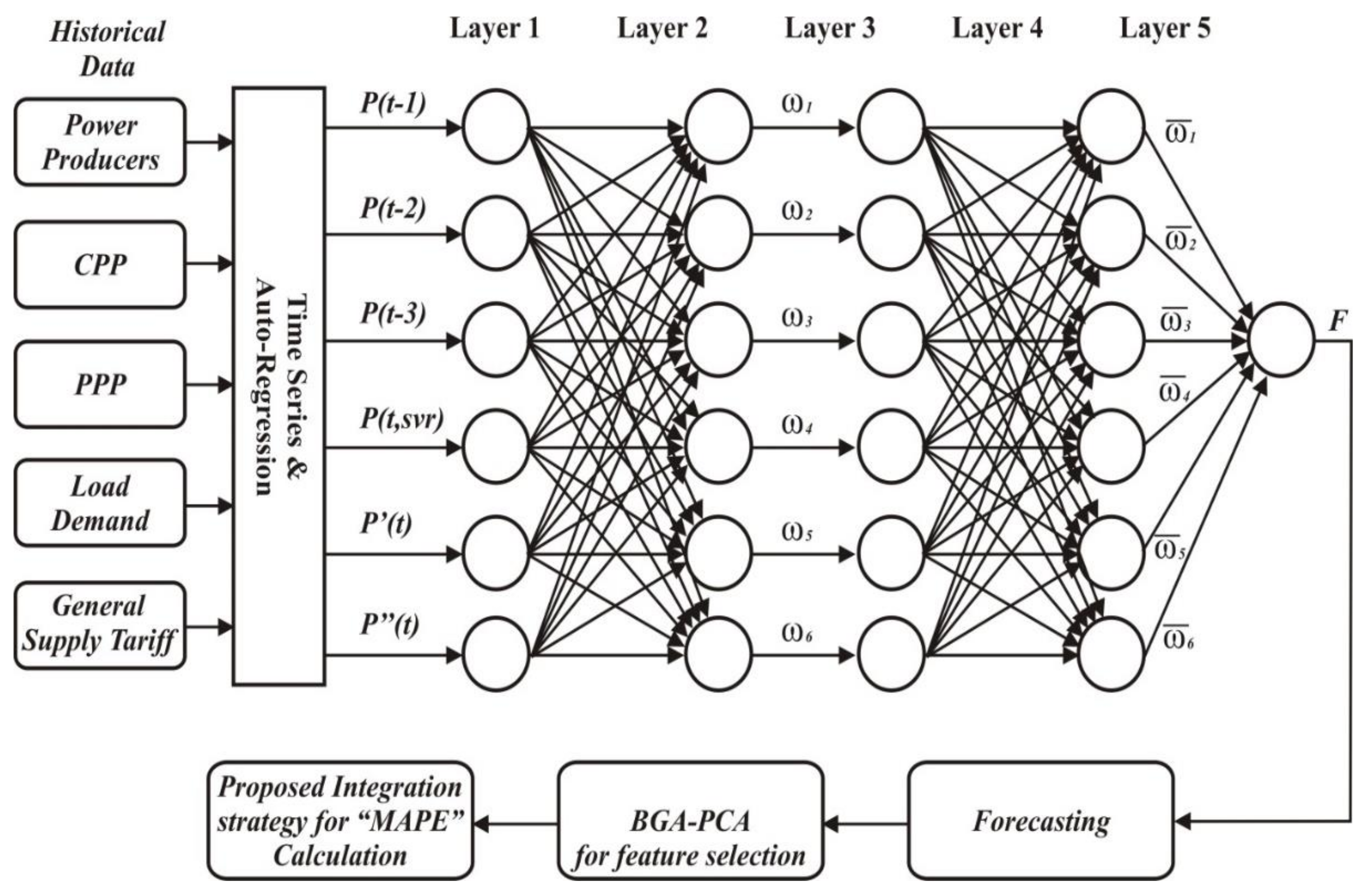
The data from NEPRA are taken for the estimation of PF for twelve months. The proposed work and Random Forest training scheme are shown in Figure 4 as systematized as follows:

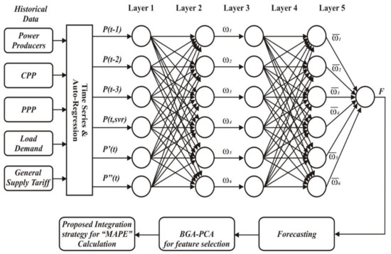
Figure 4. Flowchart of the proposed framework.

Time series and auto-regression algorithms are developed to fetch the dataset and set the objective function for proposed Equations (1)–(14). According to these equations, eight AR methods fetch the dataset by different linear and non-linear parameters.

The preprocessing of the AR method, where four types of data are fed to feedback ANFIS, contains linear data of Level-1 AR models as shown in Figure 2.

The time-series AR data have been considered an input to the proposed Feed-forward ANFIS and the overall output of Feed-forward ANFIS is computed in Equations (14)–(24). ${\overline{w}}_1$, ${\overline{w}}_2$, ${\overline{w}}_3$, ${\overline{w}}_4$, ${\overline{w}}_5$, and ${\overline{w}}_6$ are the six best weights obtained from the ANFIS model. For example, weights are ${\overline{w}}_1=60\%$, ${\overline{w}}_2=50\%$, ${\overline{w}}_3=40\%$, ${\overline{w}}_4=30\%$, ${\overline{w}}_5=20\%$, and ${\overline{w}}_6=10\%$, respectively. Then the new weights according to Equation (7) could be: ${\overline{w}}_1=\frac{60}{210}=28.5\%$, ${\overline{w}}_2=\frac{50}{210}=23.8\%$, ${\overline{w}}_3=\frac{40}{210}=19\%$, ${\overline{w}}_4=\frac{30}{210}=14.2\%$, ${\overline{w}}_5=\frac{20}{210}=9.5\%$, and ${\overline{w}}_6=\frac{10}{210}=4.7\%$. The forecasted weight according to Equations (23) and (24), where $f_n$ is the forecasting parameter of each weight according to week, weekend, month, and year, are the parameters computed in Equations (1)–(14). Assuming that $f_n$ is 30, 25, 20, 15, 10, and 5, then the forecast weights are computed as: $f=($0.28 × 30) + (0.23 × 25) + (0.19 × 20) + (0.14 × 15) + (0.09 × 10) + (0.04 × 5) ≈ 21.15. BGA-PCA for feature selection is used to eliminate the extraneous and redundant data that can improve the accuracy and reduce the computation time. The main objective of BGA is minimization as the loss function is computed in Equation (25). The BGA-PCA algorithms have removed the extra parameters, repeated terms, and irrelevant data with the given simulation parameters in Table 3.

MAPE calculation for the integration strategy is computed for each month, and the average MAPE calculation is performed in Equations (26) and (27), respectively. As per the MAPE calculation in Table 5, the MAPE of July 2019 is 5.56 as calculated from Equation (13). The weekly coefficient from different algorithms $C_i$ are 30%, 24%, 19%, 15%, 8%, and 4%. The integration strategy computed by the minimum MAPE as per Equations (28) and (29) is $MAPEofJuly2019=0.3\ast 5.56+0.24\ast 5.52+0.19\ast 5.6+0.15\ast 5.54+0.08\ast 5.59+0.04\ast 5.57=5.55$. Similarly, the MAPE of each month is calculated as given in Table 5. The flow chart of the proposed framework PF is presented in Figure 4.

PF improvement for the MAPE of each month is calculated in Table 5. The proposed model attained MAPE values of 5.56, 6.26, 4.61, 4.87, 4.94, 4.92, 4.74, 6.14, 6.27, 4.47, 6.32, and 6.41 percent for July 2019 to June 2020, respectively.

The average MAPE for 12 months computed by our proposed model is ($M_3$). Then the improvement is formulated by:

$$E_2=\frac{\left(M_2-M_3\right)}{M_3}$$

(28)

The overall improvement percentage can be calculated by:

$$E=E_1-E_2$$

(29)

Table 5. MAPE calculation for PF improvement per month.

Customer Type	Without Proposed Integration M1 MAPE Percentage	With Proposed Integration M2 MAPE Percentage	With Proposed Integration & BGA-PCA Feature Selection M3 MAPE Percentage	Percentage Overall Improvement
	Each Month MAPE %	Each Month MAPE %	Each Month MAPE %	Each Month Improvement %
July 2019	6.61	6.12	5.56	9.15%
August 2019	7.42	6.87	6.26	8.88%
September 2019	5.51	5.10	4.61	9.61%
October 2019	5.81	5.38	4.87	9.48%
November 2019	5.89	5.46	4.94	9.52%
December 2019	5.87	5.44	4.92	9.56%
January 2020	5.66	5.24	4.74	9.54%
February 2020	7.28	6.74	6.14	8.90%
March 2020	7.43	6.88	6.27	8.87%
April 2020	5.35	4.95	4.47	9.70%
May 2020	7.49	6.93	6.32	8.80%
June 2020	7.59	7.03	6.41	8.82%
Average				9.24%

Table 5. MAPE calculation for PF improvement per month.

Customer Type	Without Proposed Integration M1 MAPE Percentage	With Proposed Integration M2 MAPE Percentage	With Proposed Integration & BGA-PCA Feature Selection M3 MAPE Percentage	Percentage Overall Improvement
	Each Month MAPE %	Each Month MAPE %	Each Month MAPE %	Each Month Improvement %
July 2019	6.61	6.12	5.56	9.15%
August 2019	7.42	6.87	6.26	8.88%
September 2019	5.51	5.10	4.61	9.61%
October 2019	5.81	5.38	4.87	9.48%
November 2019	5.89	5.46	4.94	9.52%
December 2019	5.87	5.44	4.92	9.56%
January 2020	5.66	5.24	4.74	9.54%
February 2020	7.28	6.74	6.14	8.90%
March 2020	7.43	6.88	6.27	8.87%
April 2020	5.35	4.95	4.47	9.70%
May 2020	7.49	6.93	6.32	8.80%
June 2020	7.59	7.03	6.41	8.82%
Average				9.24%

5. EMS Model Evaluation

For the implementation of EMS, different kinds of loads have been selected for these buildings, as shown in Table 6. These loads are commonly used appliances in houses, industrial machines, or commercial instruments. Then the time of operation is selected by turning devices on and off in each interval.

Table 6. Power producers with CPPs, PPPs, and load demand.

	Categories		Generation (%)
Power Producers	Renewable Energy Resources		2.79%
	Hydro Power Generation		26.86%
	Gas Production		16.41%
	RLNG (RNLG)		4.46%
	Imported Coal		17.73%
	Local Coal		0.00%
	Residual fuel oil		3.09%
	Bagasse		0.84%
	Uranium		5.98%
	RNLG New		21.18%
	Imported Power		0.34%
	Mix (Captive)		0.33%
Months	Capacity Purchase Price (CPP) Per kWh	Power Purchase Price (PPP) Per kWh	Load Demand GWh
July 2019	4.58	9.44	14,275
August 2019	4.87	9.05	14,450
September 2019	5.93	9.74	13,230
October 2019	7.43	11.77	10,107
November 2019	8.96	11.91	8306
December 2019	8.60	12.54	8493
January 2020	8.24	13.86	8753
February 2020	9.45	13.47	7686
March 2020	7.85	12.95	9556
April 2020	6.84	12.94	10,974
May 2020	5.81	11.93	12,901
June 2020	5.61	11.42	13,525

Building 1

This building mainly contains household appliances as shown in Table 7. Here the first column contains the name of the load. The second contains watt rating, the third contains the probability of the on-time of the load, the fourth column contains the off time of the load, and the fifth column contains the number of times devices are turned on in each house. The percentage of generation by different power producers with CPPs, PPPs, and load demand is presented in Table 6.

Table 7. Load details of building 1.

Device Type	Hourly Consumption of Device (kW)				Number of Devices
	Watts	Start Time	Off Time	Count of Usage in a Day
Dryer	500	8	10	1	190
Dish Washer	1000	18	20	4	290
Washing Machine	1000	9	11	1	265
Oven	4000	7	22	8	280
Iron	1200	6	8	2	341
Vacuum Cleaner	1000	1	4	1	158
Fan	500	1	24	Continuous	288
Kettle	1000	5	22	4	406
Toaster	1000	7	9	2	48
Rice-Cooker	2000	10	20	2	59
Hair Dryer	1500	6	23	2	58
Blender	400	8	15	3	66
Frying Pan	1000	12	22	4	101
Coffee Maker	1500	1	24	10	56
Total					2500

Building 2

Building 2 has been selected to represent the commercial industry. This is because it contains all high-power loads. The details of loads used by consumers in building 2 are expressed in Table 8.

Table 8. Loads details of building 2.

Device Type	Hourly Consumption of Device (kW)				Number Devices
	Watts	Start Time	Off Time	Count of Usage in a Day
Water Heater	2000	1	24	Continuous	39
Welding Machine	4000	7	22	20	35
Fan/AC	1000	1	24	Continuous	16
Arc Furnace	10,000	8	20	30	8
Induction Motor	2000	1	24	20	5
DC Motor	1000	1	24	20	6
Total					109

Building 3

Building 3 has been selected as the residential building. It contains all midrange loads, as shown in Table 9. The details of the loads follow.

Table 9. Load details of building 3.

Device Type	Hourly Consumption of Device (kW)				Number Devices
	Watts	Start Time	Off Time	Count of Usage in a Day
Water Dispenser	500	1	24	10	156
Dryer	1000	8	9	2	117
Kettle	2000	7	10	5	123
Oven	4000	2	23	10	77
Coffee Maker	2000	6	14	10	99
Fan/AC	1500	1	24	Continuous	93
Air Conditioner	2000	1	24	Continuous	56
Lights	300	18	7	Continuous	87
Total					808

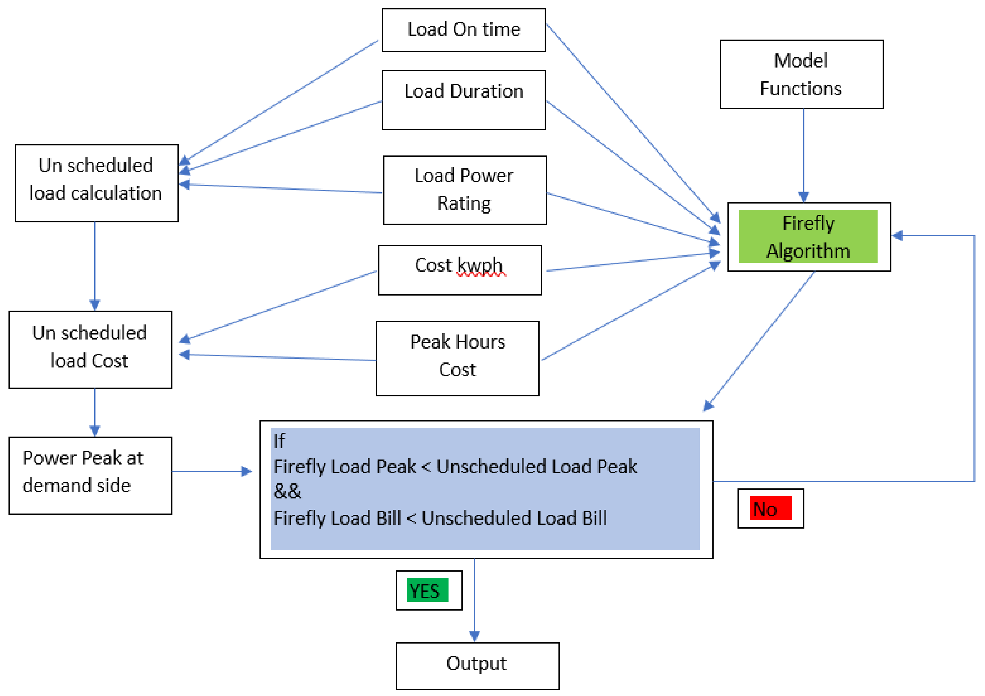
This building contains 808 devices. Therefore, to create the composite system, a large number of devices have been used. Since a large building may contain these devices, this table has been used as input data for the proposed FA. First of all, the selection of appliances is conducted, and then the following is a sequence of the algorithm as per Figure 5:

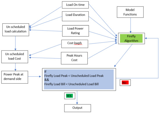
Figure 5. Illustration of the proposed firefly algorithm.

• First it captures the on-time of each appliance after initialization.
• The duration of the run-time of every appliance is the load duration.
• Load power rating is also used as input in vector form.
• Cost of electricity so that a per-month bill can be calculated. This cost varies from country to country.
• Peak hour details are also necessary. This is because peak hour cost affects three-phase connection customers, not single-phase connection customers in Pakistan. However, still, it is required because most of the users are three-phase connection customers and load on the national power grid is high at peak hours.
• All the above parameters are used as input for the FA. These variables are modeled based on model equations presented in Section 5.
• Next, the output of the firefly block is generated. It is useless until it is proven fruitful. So to create a closed-loop system, unscheduled load parameters are generated.
• Unscheduled load, cost, and peak values are calculated. These values are now compared with the firefly block if these values have two properties.
• Firefly Load Peak < Unscheduled Load Peak.
• Firefly Load Bill < Unscheduled Load Bill.
• Then, the proposed scheduling DSM is correct. If not, then the Firefly bock is again called back to recalculate parameters and reschedule the load.
• If (9) is satisfied, then the output is generated. This output contains DSM data that can be used to reduce electricity bills and power peaks in demand.

5.1. Methodology

The proposed system is based on EMS using firefly. The EMS model presented in this paper is deterministic. The basic parameters used in this paper are fixed, such as power ratings of every piece of equipment used in the houses, peak hours in which the price of all power drawn is higher, and the price of electricity.

All the appliances that cannot be controlled, for example, lights, etc., cannot be scheduled because if the duration of higher electricity cost is ongoing, users cannot turn off all their lights or the fans. The only freedom, in this case, is to turn off the lights and fans in those areas where no one is sitting, and maximum conservation policies are adopted.

The second category of the load is air conditioning appliances in which our power management and proposed techniques can be applied. These appliances can also not be shifted temporarily. Usually, there are two types of air conditioning systems. One is HVAC, and the other one is local air conditioning units installed in each house. Usually, HVAC control is difficult compared to individual units because it draws a large current and will cool an entire building even if one does not need it. However, on the other hand, the tiny air conditioning units can be used to conserve power by shifting their cooling temperature levels, and in this way, they will trip and conserve the power.

This paper considers the following vectors as considered in [47], and we modified them to design the model equation for the Firefly-based power management system proposed in this paper.

The set of appliances that can be shifted have been represented as:

$$A=\left[A_1+A_2+\cdots \dots \dots \dots \dots \dots \dots \dots \dots \dots +A_k\right]$$

(30)

The power ratings of each appliance are expressed as:

$$P=\left[P_1+P_2+\cdots \dots \dots \dots \dots \dots \dots \dots \dots \dots +P_k\right]$$

(31)

X = P/m is the power rating of each device and “m” is the number of slots per hour.

The time duration of each appliance is given as:

$$L=\left[L_1+L_2+\cdots \dots \dots \dots \dots \dots \dots \dots \dots \dots +L_k\right]$$

(32)

The point that each appliance is turned on is expressed as:

$$T_s=\left[t_1+t_{s2}+\cdots \dots \dots \dots \dots \dots \dots \dots \dots \dots +t_{sk}\right]$$

(33)

For the representation of time slots in 24 h, the following vector has been used:

$$T=\left[1+2+3+\cdots \dots \dots \dots \dots \dots \dots \dots \dots \dots +n\right]$$

(34)

The above vectors represent the model presented in this paper for EMS using the FA.

$$\mathrm{Power}\mathrm{Requirement}=\sum \mathrm{n}\notin T\sum a\notin AXn,a$$

(35)

This is a straightforward model that can be used for power optimization. To manage the peak hour issues in the proposed system, a separate vector has been created in which two elements exist as this vector as:

$$\mathrm{T}=\left[\mathrm{T}1,\mathrm{T}2\right]$$

(36)

Here, T1 = Peak Hours and T2 = Off-peak hours.

The concept of peak hours has been introduced in the proposed system to encourage people to save electricity. During peak hours, all residential users utilize electricity, and therefore, the electrical stress on the power grid increases in this time. The higher cost is applied to all the power consumed in peak hours to discourage users from turning on all high-power devices at this time.

For an electricity cost reduction for the consumers, the following model equation will be used in the proposed paper.

$$\mathrm{Total}\mathrm{Cos}\mathrm{t}\mathrm{reduction}\mathrm{in}\mathrm{Bill}={{\displaystyle \sum }}_{n=1}^{n=N}PowerRequirement—\mathrm{n}.Cn$$

(37)

So, if we minimize the above equation, then the total cost will be reduced. Here, $Cn$ represents the cost vectors, which consist of the bills of individual appliances. Now, when we schedule loads, the customer must not be dissatisfied with arrangements. So, there must be a satisfaction model. Therefore, if we minimize $\sum a\notin ADs$ (Ds = Discomfort level) then the customer will bear arrangements. So

$$Ds=\frac{\left(Ts-ast\right)}{\left(\beta end-L-ast\right)Va}\in A$$

(38)

Here, two parameters can be operated by the customer. One is the start time and the other is off time, and $\left(ast\right)$ and $\left(\beta end\right)$ are the start and end times of each appliance set by users to finish the task. Here Ts is the start time and L is the time interval for each appliance to complete the task.

The main objective is to minimize the peak load. For this purpose, the following model can be used.

$${{\displaystyle \sum }}_{n=1}^{n=N}PowerRequirement\left(Scheduled\right)<={{\displaystyle \sum }}_{n=1}^{n=N}ActualPowerRequirement$$

(39)

This means that after scheduling, the load must be less than or equal to the actual load. However, the following condition must be validated for the objective to be complete:

$$Max\left(T\ast Pscheduled\right)<Max\left(T\ast Pactual\right)$$

(40)

The above condition validates that if the scheduled power drawn is less than the actual load in peak hours, it reduces the overall cost and system capacity to handle the maximum load.

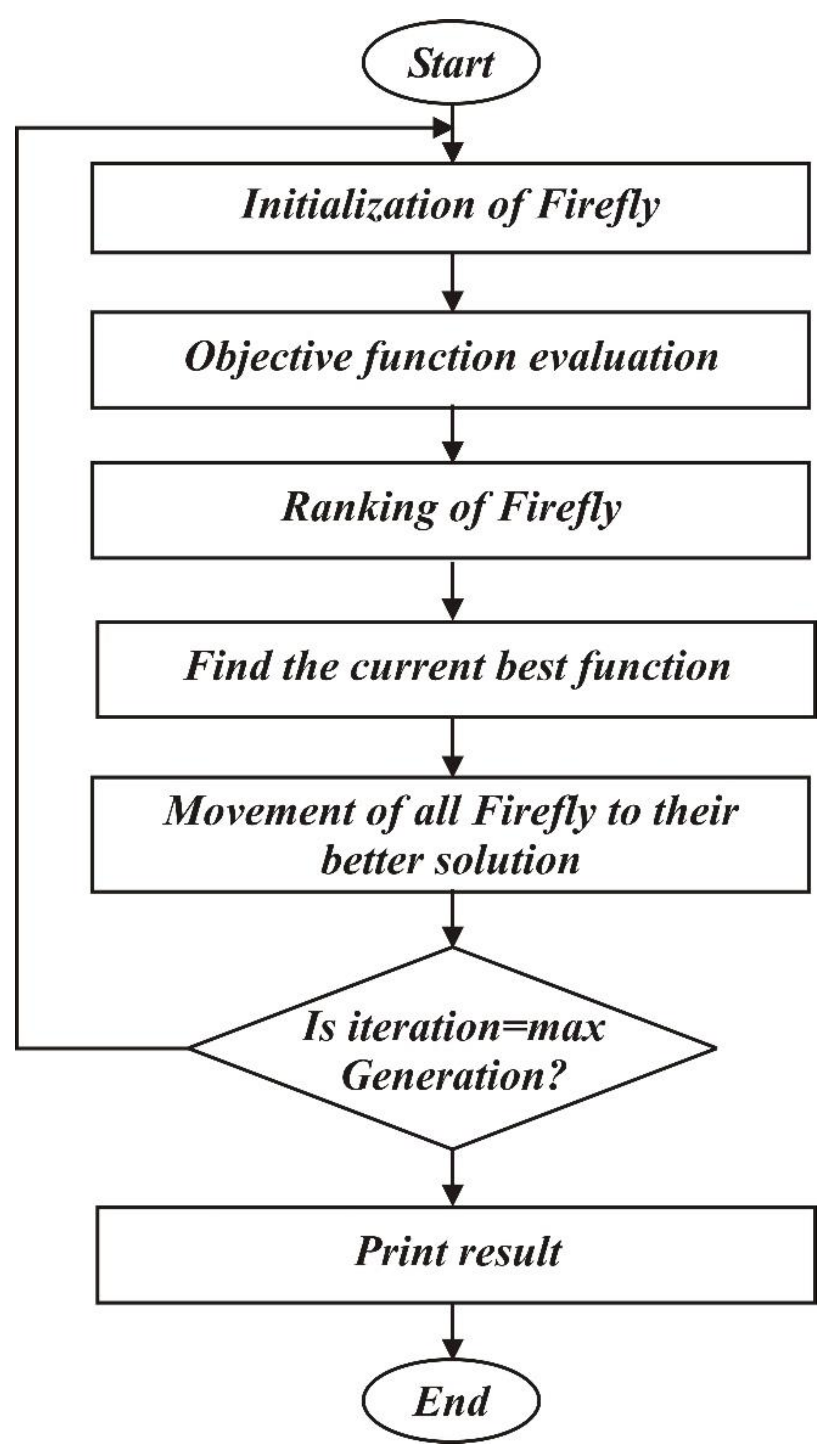
Firefly Algorithm

Xin-she-young developed FA in [48,49]. FA is a specific rule algorithm that effectively seeks the finest solution in local research. There are two basic variables of FA, namely attractiveness and emission of light. There are three basic steps followed in FA:

• At the same time, the firefly is attracted to the most attractive FA.
• In the second step, the attraction is proportional to the flashing light.
• In the last step, the coefficient value is used to control the intensity of the light.

The firefly is attracted to another firefly with a brighter flashlight than its own, as presented in [50]. An explanation of the Pseudocode of the FA can be found in [50] where the authors specify the light intensity value, initialization of light intensity, light absorption stability, and distance between two fireflies. The flowchart of FA is shown in the following Figure 6.

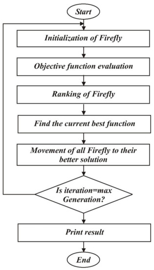
Figure 6. Flow chart of firefly algorithm.

6. Results Discussion

The MAPE of July-2019 without the proposed integration is 6.12%, and after feature selection and the proposed integration model, the MAPE is optimized to 5.56%. Thus, the overall improvement of the proposed model is 9.15%. Similarly, the MAPE of August-2019 without the proposed integration is 6.87%, and after feature selection and the proposed integration model, the MAPE is optimized to 6.26%. Thus, the overall improvement of the proposed model is 8.88%. Figure 7 illustrates the actual vs. forecasted price of electricity for July and August 2019 with an average MAPE of each month.

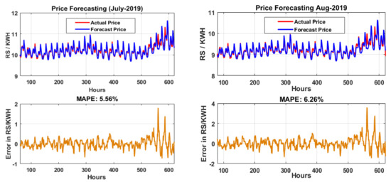
Figure 7. Actual vs. forecasted price of electricity and average MAPE for July and August 2019.

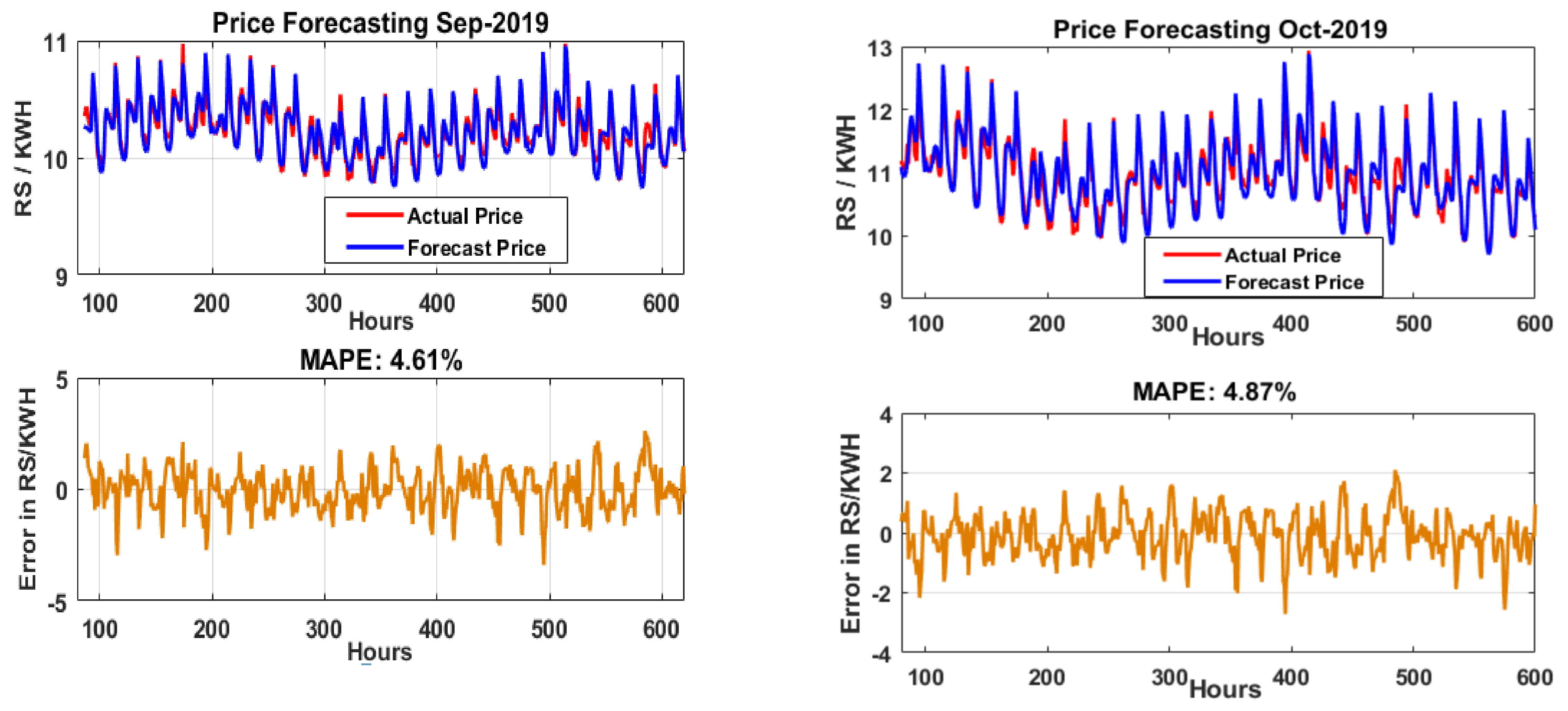
The MAPE of September-2019 without the proposed integration is 5.10%, and after feature selection and the proposed integration model, the MAPE is optimized to 4.61%. Thus, the overall improvement of the proposed model is 9.61%. The MAPE of October-2019 without the proposed integration is 5.38%, and after feature selection and the proposed integration model, the MAPE is optimized to 4.87%. Thus, the overall improvement of the proposed model is 9.48%. Figure 8 illustrates the actual vs. forecasted price of electricity for September and October 2019 with the average MAPE of each month.

Figure 8. Actual vs. forecasted price of electricity and average MAPE for September and October 2019.

The MAPE of November-2019 without the proposed integration is 5.46%; after feature selection and the proposed integration model, the MAPE is optimized to 4.94%. Thus, the overall improvement of the proposed model is 9.52%. The MAPE of December-2019 without the proposed integration is 5.44%, and after feature selection and the proposed integration model, the MAPE is optimized to 4.92%. Thus, the overall improvement of the proposed model is 9.56%. Figure 9 illustrates the actual vs. forecasted price of electricity for November and December 2019 with the average MAPE of each month.

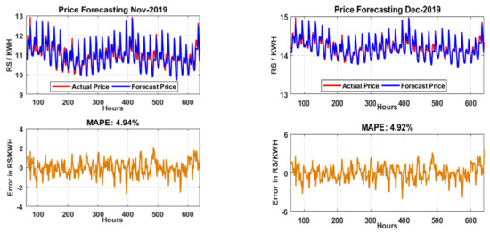
Figure 9. Actual vs. forecasted price of electricity and average MAPE for November and December 2019.

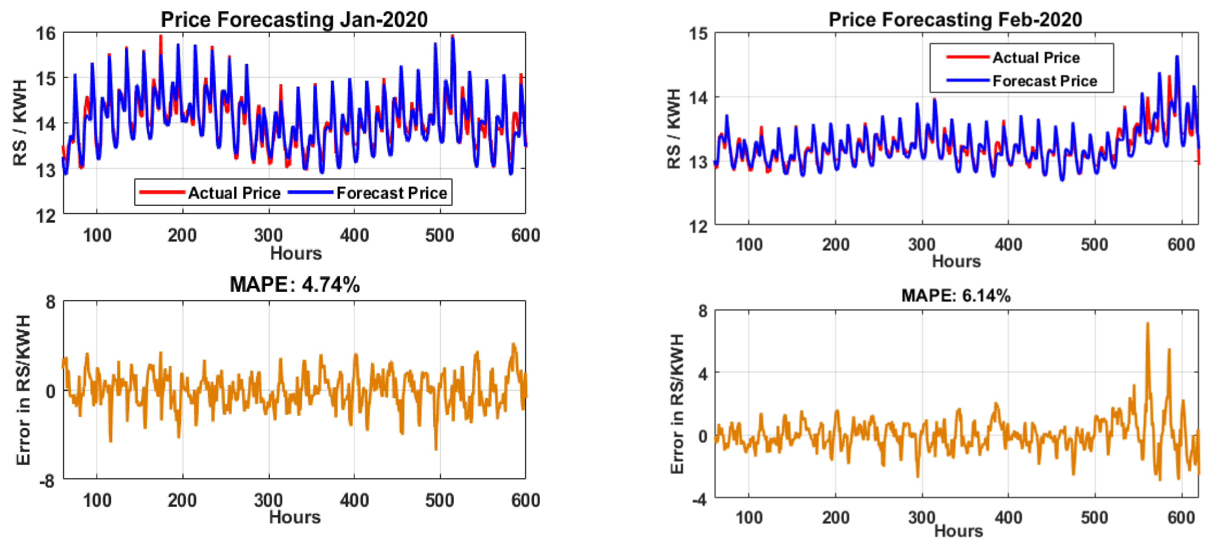
The MAPE of January-2020 without the proposed integration is 5.24%; after feature selection and the proposed integration model, the MAPE is optimized to 4.74%. Thus, the overall improvement of the proposed model is 9.54%. The MAPE of February-2020 without the proposed integration is 6.74%, and after feature selection and the proposed integration model the MAPE is optimized to 6.14%. Thus, the overall improvement of the proposed model is 8.90%. Figure 10 illustrates the actual vs. forecasted price of electricity for January and February 2020 with the average MAPE of each month.

Figure 10. Actual vs. forecasted price of electricity and average MAPE for January and February 2020.

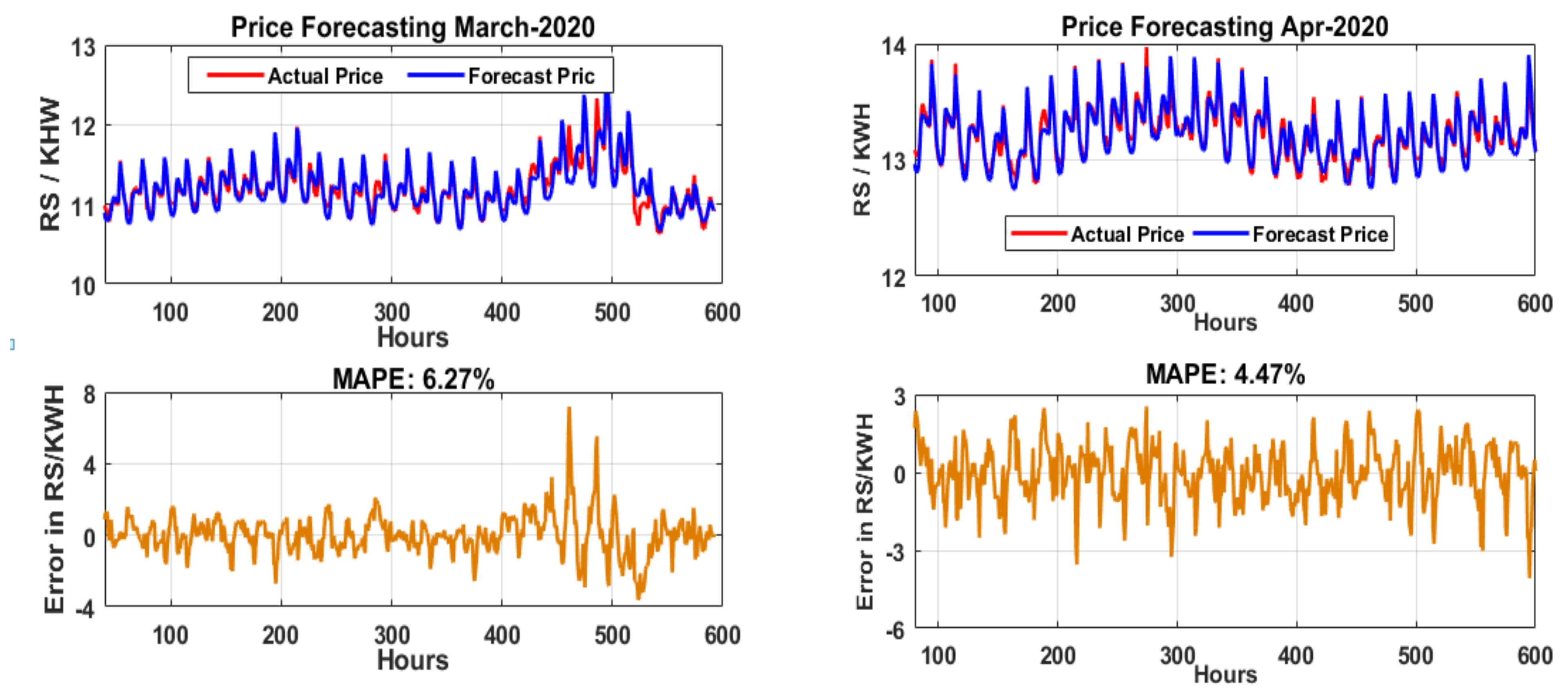
The MAPE of March-2020 without the proposed integration is 6.88%, and after feature selection and the proposed integration model, the MAPE is optimized to 6.27%. Thus, the overall improvement of the proposed model is 8.87%. The MAPE of April-2020 without the proposed integration is 4.95%, and after feature selection and the proposed integration model, the MAPE is optimized to 4.47%. Thus, the overall improvement of the proposed model is 9.70%. Figure 11 illustrates the actual vs. forecasted price of electricity for March and April 2020 with an average MAPE of each month.

Figure 11. Actual vs. forecasted price of electricity and average MAPE for March and April 2020.

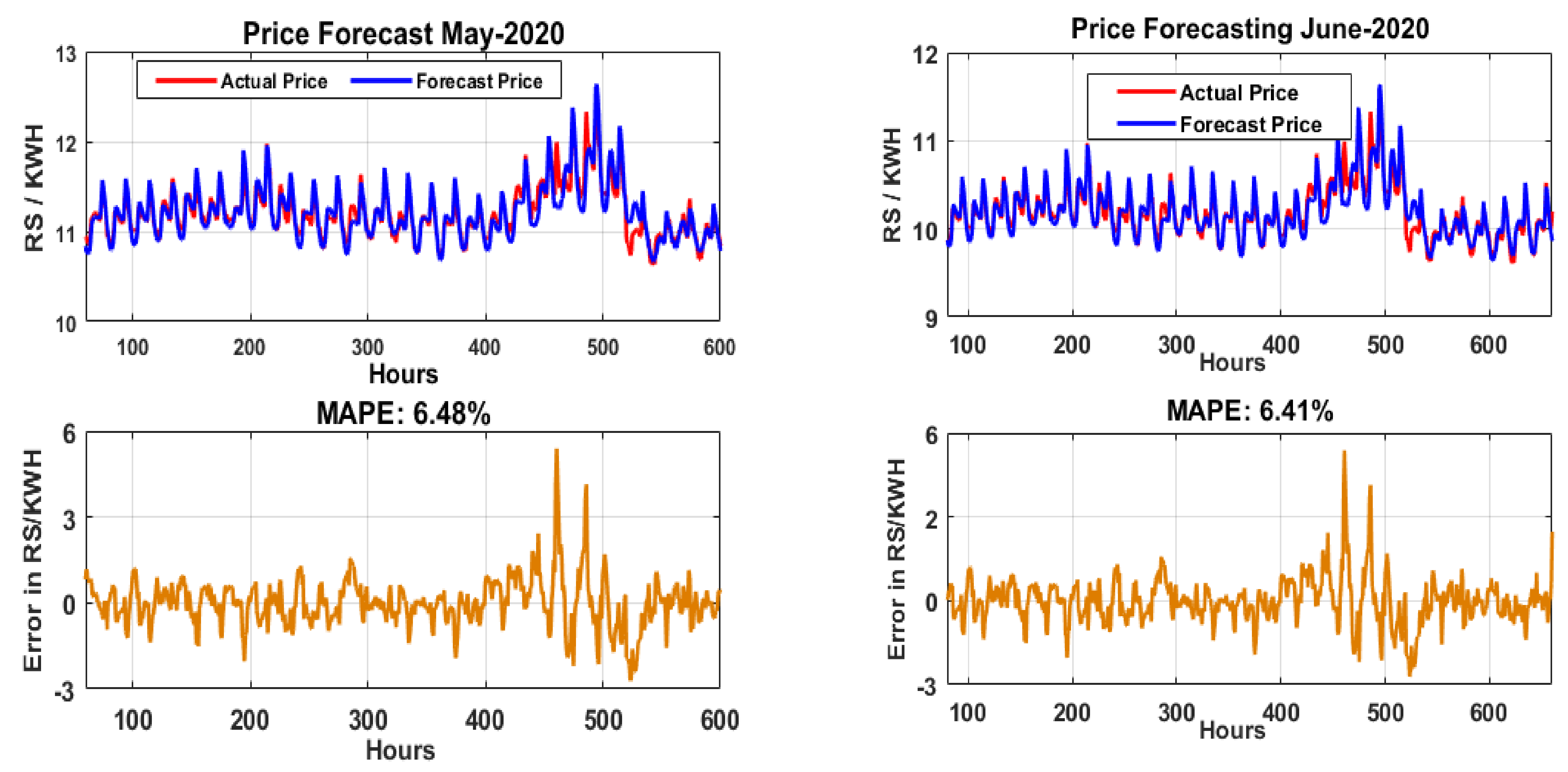
The MAPE of May-2020 without the proposed integration is 6.93%, and after feature selection and the proposed integration model, the MAPE is optimized to 6.32%. Thus, the overall improvement of the proposed model is 8.80%. The MAPE of June-2020 without the proposed integration is 7.03%, and after feature selection and the proposed integration model, the MAPE is optimized to 6.41%. Thus, the overall improvement of the proposed model is 8.82%. Figure 12 illustrates the actual vs. forecasted price of electricity for May and June 2020 with an average MAPE of each month.

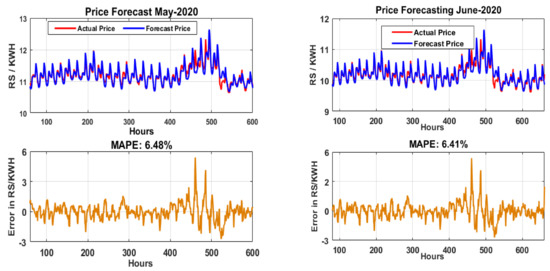
Figure 12. Actual vs. forecasted price of electricity and average MAPE for May and June 2020.

In this section, the proposed system is discussed. This paper presented the FA-based EMS technique and achieved all the objectives.

7. Results of Energy Management System

7.1. Tariff Plan

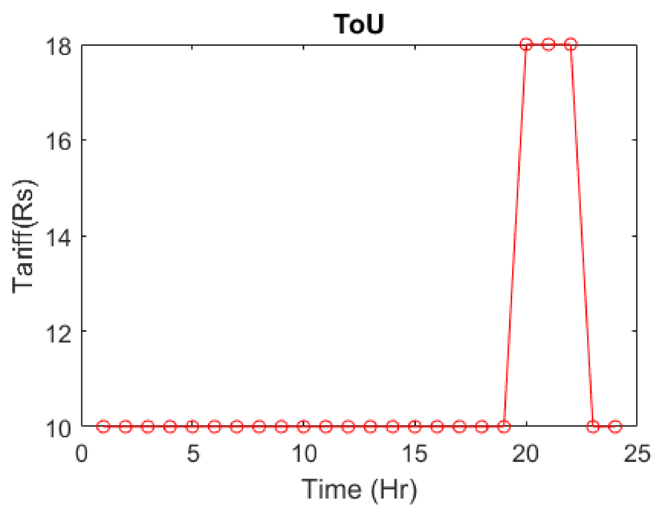
Figure 13 presents the overview of the FA regarding the cost of electricity related to its time slot. Here, the two-stage tariff plan has been used.

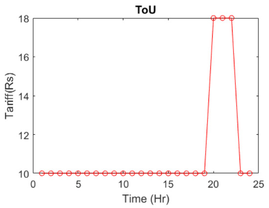
Figure 13. Tariff plan implemented in the proposed system for different time slots.

Figure 13 shows the tariff plan implemented in the proposed system. The y-axis shows the tariff rate in Pkr and the x-axis shows the time slots. It is a standard two-level tariff plan. In 24 h, approximately 3 to 4 h are considered peak hours, from 7 pm to 11:00 p.m. In these peak hours, the price is approximately double. Due to this, all consumers utilize maximum appliances at this stage. Therefore, electricity demand is also higher at this time. To encourage power conservation, these tariff plans have been introduced so that in peak hours’, customers must conserve electricity so that the cost of electricity and electrical stress on the national grid can be reduced.

7.2. Load Management

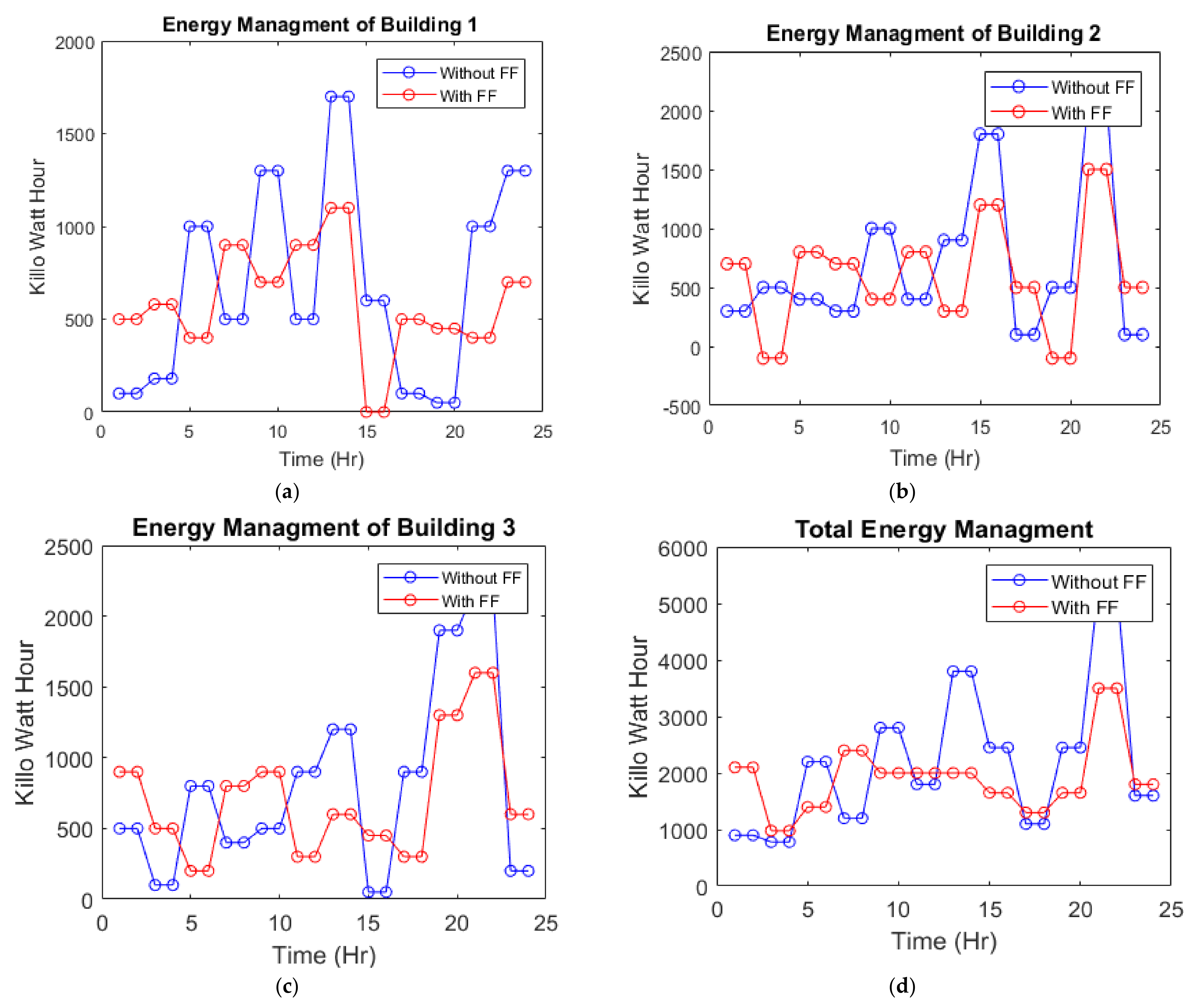
Figure 14a presents the energy management of building 1 with and without FF. The y-axis shows the power consumption in kilowatt-hour and the x-axis shows the time slots. Here, the blue line represents the unscheduled load, while the red line is the scheduled load with firefly. In this graph, peak load has shifted from 1700 kw to 1100 kw. It reduces the peak load by 35%. It will also reduce the demand for power source capacity.

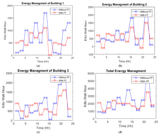
Figure 14. Energy management with and without FF for: (a) Building-1, (b) Building-2, (c) Building-3, (d) all buildings.

Figure 14b illustrates the energy management of building 2 with and without FF. The y-axis shows the power consumption in kilowatt-hour, and the x-axis shows the time slots. Here, the peak of the load was at 2100 kw, but the proposed system shifted it to 1600 kw. So, in building 2, an overall 24% reduction in peak load has been observed. Figure 14c shows the energy management of building 3 with and without FF. The y-axis shows the power consumption in kilowatt-hour, and the x-axis shows the time slots. Here it can be seen that the maximum peak in building 3 occurs at 2300 kw. Therefore, the proposed system rescheduled the load and shifted it to 1600 kw. This is a 30% reduction in peak demand. Figure 14d exhibits the total energy management of all buildings and the objective of the proposed system. The y-axis shows the power consumption of all buildings in kilowatt-hour and the x-axis shows the time slots. Here, the unscheduled load is blue, while the second graph is an FA-based managed graph. As discussed earlier, the main objectives of the proposed system are to reduce the electricity cost and trigger peak reduction. The figure clearly explains that unscheduled load has various peaks. So, it has a higher cost per kilowatt-hour. However, the FA has managed this unscheduled load in such a way that its peaks are reduced.

Although some of the load peaks are greater than the unscheduled load, the overall effect of the proposed system has reduced the electricity cost. An unscheduled load requires a 5400 KW power source, while a DSM-based load requires only a 3500 KW source. This means a total 35% peak reduction has occurred. Furthermore, cost and electrical stress on the national grid have been reduced.

7.3. Per Day Electricity Bill

Figure 15a presents the power cost comparison of building 1. The purple color represents a firefly-based scheduled load in this graph, while the black colored bar represents an unscheduled load. It is visible that FA reduced the cost of electricity per day from 190,000 Rs to 150,000 Rs, which is a 21% reduction in the bill for building 1. Figure 15b shows the power cost comparison of building 2. The y-axis shows the cost, and the x-axis shows the time slots. It is visible that FA reduced the cost of electricity per day from 210,000 Rs to 170,000 Rs, which is a 19% reduction in the per-day bill. Figure 15c illustrates the power cost comparison of building 3. The y-axis shows the cost and the x-axis shows the time slots. It is visible that FA has reduced the cost of electricity per day from 250,000 Rs to 200,000 Rs, which is a 20% reduction in the bill for building 3. Figure 15d presents the cost of electricity of three buildings in a single day. The y-axis shows the cost and the x-axis shows the time slots. The application of the proposed system for the DSM reduced the electricity cost from 650,000 Rs to 520,000 Rs approximately, which is approximately a 20% cost reduction and power saving.

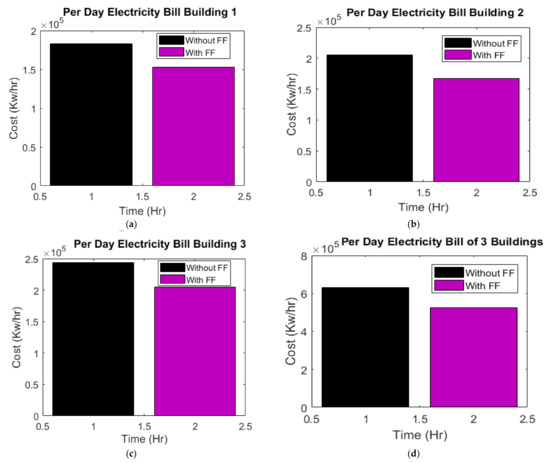
Figure 15. Power cost comparison with and without FF for (a) Building-1, (b) Building-2, (c) Building-3, (d) all buildings.

8. Conclusions and Future Studies

PF is a crucial aspect for better planning and operation of power generation systems, as is the EMS proposed in the second part of the paper. A new combinational forecasting model based on time-series and auto-regression algorithms, ML-based feedback ANFIS, and a BGA-PCA algorithm is proposed for the best feature selection. This paper presents a novel time-series and auto-regression algorithm for analyzing the larger and more complex historical data. The time-series AR model is further validated by the ML-based feedback ANFIS model, where eight stages are computed. The BGA-PCA approach for attaining the best feature selection is evaluated and attained more optimized results. A remarkable improvement in MAPE of less than 10% in overall performance and an average MAPE of 9.24 has been achieved by a proposed integration that is significantly improved compared to previous ones. This model can optimize the performance of power grids by predicting the optimized PF and can overcome the problems related to the planning and operation of the smart grid.

Price and load forecasting are considered the main features of the revolutionary smart grid system, which helps to enhance electricity generation in a decentralized grid network. Providing reliable and uninterruptable electricity supply during peak hours facilitates the generation system by providing essential information on load and price forecasting. Therefore, this paper has made an effort to minimize peak load demand by load and PF analysis through the Machine-Learning approach.

References

- Stone, P.; Brooks, R.; Brynjolfsson, E.; Calo, R.; Etzioni, O.; Hager, G.; Hirschberg, J.; Kalyanakrishnan, S.; Kamar, E.; Kraus, S.; et al. Artificial Intelligence and Life in 2030: The One Hundred Year Study on Artificial Intelligence; Stanford University: Stanford, CA, USA, 2016. [Google Scholar]
- Macedo, M.; Galo, J.; de Almeida, L.; Lima, A.D.C. Demand side management using artificial neural networks in a smart grid environment. Renew. Sustain. Energy Rev. 2015, 41, 128–133. [Google Scholar] [CrossRef]
- Ahmad, A.; Khan, A.; Javaid, N.; Hussain, H.M.; Abdul, W.; Almogren, A.; Alamri, A.; Niaz, I.A. An Optimized Home Energy Management System with Integrated Renewable Energy and Storage Resources. Energies 2017, 10, 549. [Google Scholar] [CrossRef] [Green Version]
- Logenthiran, T.; Srinivasan, D.; Shun, T.Z. Demand Side Management in Smart Grid Using Heuristic Optimization. IEEE Trans. Smart Grid 2012, 3, 1244–1252. [Google Scholar] [CrossRef]
- Khan, M.A.; Javaid, N.; Mahmood, A.; Khan, Z.A.; Alrajeh, N. A generic demand-side management model for smart grid. Int. J. Energy Res. 2015, 39, 954–964. [Google Scholar] [CrossRef]
- Moon, S.; Lee, J.-W. Multi-Residential Demand Response Scheduling with Multi-Class Appliances in Smart Grid. IEEE Trans. Smart Grid 2016, 9, 2518–2528. [Google Scholar] [CrossRef]
- Remani, T.; Jasmin, E.A.; Ahamed, T.I. Residential Load Scheduling with Renewable Generation in the Smart Grid: A Reinforcement Learning Approach. IEEE Syst. J. 2018, 13, 3283–3294. [Google Scholar] [CrossRef]
- Masood, B.; Khan, M.A.; Baig, S.; Song, G.; Rehman, A.U.; Rehman, S.U.; Asif, R.M.; Rasheed, M.B. Investigation of Deterministic, Statistical and Parametric NB-PLC Channel Modeling Techniques for Advanced Metering Infrastructure. Energies 2020, 13, 3098. [Google Scholar] [CrossRef]
- Liu, D.; Xiao, J.; Liu, J.; Yuan, X.; Zhang, S. Dynamic Energy Trading and Load Scheduling Algorithm for the End-User in Smart Grid. IEEE Access 2020, 8, 189632–189645. [Google Scholar] [CrossRef]
- Siddique, M.A.B.; Asad, A.; Asif, R.M.; Rehman, A.U.; Sadiq, M.T.; Ullah, I. Implementation of Incremental Conductance MPPT Algorithm with Integral Regulator by Using Boost Converter in Grid-Connected PV Array. IETE J. Res. 2021, 1–14. [Google Scholar] [CrossRef]
- Mahmood, T.; Ullah, K.; Khan, Q.; Jan, N. An approach toward decision-making and medical diagnosis problems using the concept of spherical fuzzy sets. Neural Comput. Appl. 2018, 31, 7041–7053. [Google Scholar] [CrossRef]
- Costanzo, G.T.; Zhu, G.; Anjos, M.F.; Savard, G. A System Architecture for Autonomous Demand Side Load Management in Smart Buildings. IEEE Trans. Smart Grid 2012, 3, 2157–2165. [Google Scholar] [CrossRef]
- Long, K.; Yang, Z. Model predictive control for household energy management based on individual habit. In Proceedings of the 2013 25th Chinese Control and Decision Conference (CCDC), Guiyang, China, 25–27 May 2013; pp. 3676–3681. [Google Scholar]
- Stavrakas, V.; Flamos, A. A modular high-resolution demand-side management model to quantify benefits of demand-flexibility in the residential sector. Energy Convers. Manag. 2019, 205, 112339. [Google Scholar] [CrossRef]
- Yoon, J.H.; Baldick, R.; Novoselac, A. Dynamic Demand Response Controller Based on Real-Time Retail Price for Residential Buildings. IEEE Trans. Smart Grid 2014, 5, 121–129. [Google Scholar] [CrossRef]
- Agarwal, A.; Ojha, A.; Tewari, S.C.; Tripathi, M.M. Hourly load and price forecasting using ANN and fourier analysis. In Proceedings of the 2014 6th IEEE Power India International Conference (PIICON), Delhi, India, 5–7 December 2014; pp. 1–6. [Google Scholar]
- Rehman, A.U.; Naqvi, R.A.; Rehman, A.; Paul, A.; Sadiq, M.T.; Hussain, D. A Trustworthy SIoT Aware Mechanism as an Enabler for Citizen Services in Smart Cities. Electronics 2020, 9, 918. [Google Scholar] [CrossRef]
- Jahangir, H.; Tayarani, H.; Baghali, S.; Ahmadian, A.; Elkamel, A.; Golkar, M.A.; Castilla, M. A Novel Electricity Price Forecasting Approach Based on Dimension Reduction Strategy and Rough Artificial Neural Networks. IEEE Trans. Ind. Inform. 2019, 16, 2369–2381. [Google Scholar] [CrossRef]
- Siddique, M.A.B.; Khan, M.A.; Asad, A.; Rehman, A.U.; Asif, R.M.; Rehman, S.U. Maximum Power Point Tracking with Modified Incremental Conductance Technique in Grid-Connected PV Array. In Proceedings of the 2020 5th International Conference on Innovative Technologies in Intelligent Systems and Industrial Applications (CITISIA), Sydney, Australia, 25–27 November 2020; pp. 1–6. [Google Scholar]
- Kristiansen, T. Forecasting Nord Pool day-ahead prices with an autoregressive model. Energy Policy 2012, 49, 328–332. [Google Scholar] [CrossRef]
- Abedinia, O.; Amjady, N.; Zareipour, H. A New Feature Selection Technique for Load and Price Forecast of Electrical Power Systems. IEEE Trans. Power Syst. 2016, 32, 62–74. [Google Scholar] [CrossRef]
- Alanis, A.Y. Electricity Prices Forecasting Using Artificial Neural Networks. IEEE Lat. Am. Trans. 2018, 16, 105–111. [Google Scholar] [CrossRef]
- Al-Awami, A.T.; Amleh, N.A.; Muqbel, A.M. Optimal Demand Response Bidding and Pricing Mechanism With Fuzzy Optimization: Application for a Virtual Power Plant. IEEE Trans. Ind. Appl. 2017, 53, 5051–5061. [Google Scholar] [CrossRef]
- Elattar, E.E.; Elsayed, S.K.; Farrag, T.A. Hybrid Local General Regression Neural Network and Harmony Search Algorithm for Electricity Price Forecasting. IEEE Access 2020, 9, 2044–2054. [Google Scholar] [CrossRef]
- Mosbah, H.; El-Hawary, M. Hourly Electricity Price Forecasting for the Next Month Using Multilayer Neural Network. Can. J. Electr. Comput. Eng. 2016, 39, 283–291. [Google Scholar] [CrossRef]
- Asif, R.M.; Rehman, A.U.; Rehman, S.U.; Arshad, J.; Hamid, J.; Sadiq, M.T.; Tahir, S. Design and analysis of robust fuzzy logic maximum power point tracking based isolated photovoltaic energy system. Eng. Rep. 2020, 2, e12234. [Google Scholar] [CrossRef]
- Schnürch, S.; Wagner, A. Electricity Price Forecasting with Neural Networks on EPEX Order Books. Appl. Math. Financ. 2020, 27, 189–206. [Google Scholar] [CrossRef]
- Usman, M.; Khan, Z.A.; Khan, I.U.; Javaid, S.; Javaid, N. Data Analytics for Short Term Price and Load Forecasting in Smart Grids using Enhanced Recurrent Neural Network. In Proceedings of the 2019 Sixth HCT Information Technology Trends (ITT), Ras Al Khaimah, United Arab Emirates, 20–21 November 2019; pp. 84–88. [Google Scholar]
- Lee, D.; Shin, H.; Baldick, R. Bivariate Probabilistic Wind Power and Real-Time Price Forecasting and Their Applications to Wind Power Bidding Strategy Development. IEEE Trans. Power Syst. 2018, 33, 6087–6097. [Google Scholar] [CrossRef]
- Sahay, K.B.; Tripathi, M.M. Day ahead hourly load forecast of PJM electricity market and ISO New England market by using artificial neural network. In Proceedings of the 2013 IEEE Innovative Smart Grid Technologies-Asia (ISGT Asia), Washington, DC, USA, 19–22 February 2014; pp. 1–5. [Google Scholar]
- Upadhyay, K.; Tripathi, M.; Singh, S. An approach to short term load forecasting using market price signal. In Proceedings of the 19th International Conference on Electricity Distribution, Vienna, Austria, 21–24 May 2007. [Google Scholar]
- Cau, G.; Cocco, D.; Petrollese, M.; Kær, S.K.; Milan, C. Energy management strategy based on short-term generation scheduling for a renewable microgrid using a hydrogen storage system. Energy Convers. Manag. 2014, 87, 820–831. [Google Scholar] [CrossRef]
- Lv, T.; Ai, Q. Interactive energy management of networked microgrids-based active distribution system considering large-scale integration of renewable energy resources. Appl. Energy 2016, 163, 408–422. [Google Scholar] [CrossRef]
- Shewale, A.; Mokhade, A.; Funde, N.; Bokde, N.D. An Overview of Demand Response in Smart Grid and Optimization Techniques for Efficient Residential Appliance Scheduling Problem. Energies 2020, 13, 4266. [Google Scholar] [CrossRef]
- Zhao, B.; Xue, M.; Zhang, X.; Wang, C.; Zhao, J. An MAS based energy management system for a stand-alone microgrid at high altitude. Appl. Energy 2015, 143, 251–261. [Google Scholar] [CrossRef] [Green Version]
- Xiao, J.; Wang, P.; Setyawan, L.; Xu, Q. Multi-Level Energy Management System for Real-Time Scheduling of DC Microgrids with Multiple Slack Terminals. IEEE Trans. Energy Convers. 2015, 31, 392–400. [Google Scholar] [CrossRef]
- Farzan, F.; Jafari, M.A.; Masiello, R.; Lu, Y. Toward Optimal Day-Ahead Scheduling and Operation Control of Microgrids Under Uncertainty. IEEE Trans. Smart Grid 2014, 6, 499–507. [Google Scholar] [CrossRef]
- Rehman, A.U.; Aslam, S.; Abideen, Z.U.; Zahra, A.; Ali, W.; Junaid, M.; Javaid, N. Efficient Energy Management System Using Firefly and Harmony Search Algorithm. In International Conference on Broadband and Wireless Computing, Communication and Applications, Spain, 8–10 November 2017; Springer: Cham, Switzerland, 2017; pp. 37–49. [Google Scholar] [CrossRef]
- Saba, A.; Khalid, A.; Ishaq, A.; Parvez, K.; Aimal, S.; Ali, W.; Javaid, N. Home Energy Management Using Firefly and Harmony Search Algorithm. In Proceedings of the 12th International Conference on P2P, Parallel, Grid, Cloud and Internet Computing, Barcelona, Spain, 8–10 November 2017. [Google Scholar]
- Oladeji, O.; Olakanmi, O.O. A genetic algorithm approach to energy consumption scheduling under demand response. In Proceedings of the 2014 IEEE 6th International Conference on Adaptive Science & Technology (ICAST), Ota, Nigeria, 29–31 October 2014. [Google Scholar] [CrossRef]
- Asgher, U.; Rasheed, M.B.; Al-Sumaiti, A.S.; Ur-Rahman, A.; Ali, I.; Alzaidi, A.; Alamri, A. Smart Energy Optimization Using Heuristic Algorithm in Smart Grid with Integration of Solar Energy Sources. Energies 2018, 11, 3494. [Google Scholar] [CrossRef] [Green Version]
- Latifi, M.; Khalili, A.; Rastegarnia, A.; Zandi, S.; Bazzi, W. A distributed algorithm for demand-side management: Selling back to the grid. Heliyon 2017, 3, e00457. [Google Scholar] [CrossRef]
- Ahmed, A.; Manzoor, A.; Khan, A.; Zeb, A.; Madni, H.A.; Qasim, U.; Khan, Z.A.; Javaid, N. Performance Measurement of Energy Management Controller Using Heuristic Techniques. In Complex, Intelligent, and Software Intensive Systems, Proceedings of the Conference on Complex, Intelligent, and Software Intensive Systems, Turin, Italy, 10–13 July 2017; Springer: Cham, Switzerland, 2017; Volume 611, pp. 181–188. [Google Scholar] [CrossRef]
- Kilimci, Z.H.; Akyuz, A.O.; Uysal, M.O.; Akyokus, S.; Bulbul, B.A.; Ekmis, M.A. An Improved Demand Forecasting Model Using Deep Learning Approach and Proposed Decision Integration Strategy for Supply Chain. Complexity 2019, 2019, 9067367. [Google Scholar] [CrossRef] [Green Version]
- Jadidi, A.; Menezes, R.; De Souza, N.; Lima, A.C.D.C.; Souza, D.; Lima, D.C. Short-Term Electric Power Demand Forecasting Using NSGA II-ANFIS Model. Energies 2019, 12, 1891. [Google Scholar] [CrossRef] [Green Version]
- Yousaf, A.; Asif, R.; Shakir, M.; Rehman, A.; Adrees, M.S. An Improved Residential Electricity Load Forecasting Using a Machine-Learning-Based Feature Selection Approach and a Proposed Integration Strategy. Sustainability 2021, 13, 6199. [Google Scholar] [CrossRef]
- Bayat, P.; Monjezi, M.; Rezakhah, M.; Armaghani, D.J. Artificial Neural Network and Firefly Algorithm for Estimation and Minimization of Ground Vibration Induced by Blasting in a Mine. Nat. Resour. Res. 2020, 29, 4121–4132. [Google Scholar] [CrossRef]
- Yang, X.S.; He, X. Firefly algorithm: Recent advances and applications. Int. J. Swarm Intell. 2013, 1, 36–50. [Google Scholar] [CrossRef] [Green Version]
- Yang, X.S. Firefly algorithms for multimodal optimization. In Proceedings of the Lecture Notes in Computer Science (Including Subseries Lecture Notes in Artificial Intelligence and Lecture Notes in Bioinformatics), Suzhou, China, 2–4 April 2009; Volume 5792 LNCS, pp. 169–178. [Google Scholar]
- Zhang, L.; Liu, L.; Yang, X.-S.; Dai, Y. A Novel Hybrid Firefly Algorithm for Global Optimization. PLoS ONE 2016, 11, e0163230. [Google Scholar] [CrossRef] [Green Version]
Publisher’s Note: MDPI stays neutral with regard to jurisdictional claims in published maps and institutional affiliations. |
© 2021 by the authors. Licensee MDPI, Basel, Switzerland. This article is an open access article distributed under the terms and conditions of the Creative Commons Attribution (CC BY) license (https://creativecommons.org/licenses/by/4.0/).