Abstract
The main focuses of the Sino–US trade dispute are the issue of trade interests. If taking environmental costs into consideration, the trade interests are even more overestimated. There are different methods for measuring trade interests, and the results obtained under different methods differ. This paper uses the gross trade, value-added trade and value-added-in trade framework to calculate the economic gains and correspondent embodied pollution in China–US trade, compares the differences in results under different models and makes possible explanations. Our conclusions are as follows: (1) Traditional gross trade statistics have overestimated China’s economic benefits. The trade balance in gross trade was overestimated by 35% and 40% compared to the value-added trade and value-added-in trade. (2) China was a net exporter of embodied pollution and paid huge environmental costs from 1995 to 2011. (3) China’s exports are environmentally worse than the United States, and the calculation of pollution terms of trade proves that China paid a greater environmental cost for the same amount of economic benefits. (4) Different accounting frameworks have a great impact on the embodied pollution results at the industry level. Pollution based on value-added trade was more concentrated. The major polluting industries also changed.
1. Introduction
Trade disputes between China and the United States have become the center of public attention in recent years. According to the World Bank, China–US trade surplus hit a record high of $323.3 billion in 2018. The United States believes that China’s trade surplus with the US was caused by “unfair trade practices” and intellectual property theft, and they set tariffs and other trade barriers on China. However, it would be premature to draw a conclusion on gains and losses in Sino–US trade.
Traditional trade statistics quantifies the value of trade according to the gross terms (the gross value of products). Using it as a gauge for economic gains in trade would “double count” goods traded cross borders and fail to distinguish the value contributed by particular country. There are discrepancies between the real contributions in trade and traditional trade statistics [1,2]. In addition, under the background of global value chain (GVC) division of production, developing countries tend to engage in the downstream end of production chains characterized by high energy consumption and high pollution. Developing countries are more likely to bear the cost of environmental damages [3,4].
It is necessary to re-examine the real gains and losses in Sino–US trade. Studies have shown that China has maintained a trade surplus at the cost of huge environmental losses [5,6].Environmental damages should not be excluded when discussing gains and losses in trade. It is reasonable to assume that gains and losses in Sino–US trade may change after taking account of pollution emission. Trade in gross terms, trade in value added and value-added-in trade were used as different gauges of economic gains in trade. The use of different accounting frameworks may cause differences in conclusions.
Considering environmental costs, we use models of gross value trade, value-added trade and value-added-in trade to re-examine the economic gains and correspondent embodied pollution in China–US trade, compare the differences in results among different models and make possible explanations. SO and NO are chosen as the proxies for environmental costs as their environmental impacts are regional [7] and, compared to carbon dioxide (CO), they seldom involve complex emission liability on which the academic community has not yet reached a consensus [8,9].
We narrow the scope of research to merchandise trade to answer current international disputes in a targeted manner. In addition, we use and improve Pollution Terms of Trade (PTT) [10] and the pollution intensity in value-added Exports (PIE) [11] to show a more complete picture of a country’s economic–environmental position in trade.
This article attempts to make incremental contributions from the following aspects. First, most of the existing studies focused on economic gains or carbon emissions, and they seldom investigated both the economic benefits and environmental costs in bilateral trade [11,12]. Second, many studies on environmental costs targeted embodied CO, and embodied pollution in trade is relatively rare to be studied and needs to be further explored. Third, different accounting frameworks have been applied by scholars, but few studies have indicated the possible impacts on calculating results. In particular, studies on the impacts at the level of bilateral trade are almost blank. Finally, this article expands the corresponding PIE and PTT indexes based on the above models, links the two indexes and comprehensively evaluates the economic–environmental status of China and the United States to reveal the actual gains and losses in Sino–US trade.
2. Literature Review
2.1. Gross Trade, Value Added Trade and Value Added in Trade
As official trade statistics measured in gross terms “double counts” the value of intermediate goods and is inconsistent with System of National Accounts (SNA), this at least implicitly signifies that official trade statistics could not truly reflect the economic gains in trade. Case studies are done to figure out who produces for whom and how much contribution each stage of production makes [13,14]. Intuitive, subtle and insightful as such case study approaches are, they cannot completely trace the value-added contained in the product, let alone the value added in a country’s trade.
In order to better clarify the economic benefits and vertical specialization in international trade, some measures have been proposed and calculation methods have been developed. Daudin et al. [15] suggested using value-added trade as a new measure of international trade. Johnson and Noguera [16] constructed a global bilateral input–output table to calculate the value added content in bilateral trade and put forward the VAX ratio (value added to gross exports) as a measurement of the intensity of production sharing.
Stehrer [17] indicated that the concepts of trade in value added and value-added-in trade are different. The former focuses on value-added-in trade, while the latter focuses on the distribution of benefits in gross trade. Koopman et al. [18] provided a mathematical framework to decompose gross exports into nine parts, distinguished among domestic value added, foreign value added and double counted parts. Wang et al. [19] proposed a method to further decompose the gross trade at the sector, bilateral or bilateral-sector level.
Thus far, there are relatively mature calculation methods for gross trade, value-added trade and value-added-in trade and some scholars studied the differences between trade in value added and value-added-in trade. Stehrer [17] empirically found that trade in value added and value-added-in trade are equal when calculating overall net trade of a country; however, this is not the case in bilateral trade.
Scholars have compared the differences in gross trade and value-added trade empirically by bilateral trade study. Kordalska and Olczyk [20] studied the impact of determinants on service exports in value added terms and in gross terms and found that their impacts were quite similar but the strength of impact may differ. Wang and Sheng [21] measured the trade balances in Sino–US trade from 1995 to 2009 in value added terms and compared it with traditional trade statistics and found that traditional trade statistics overestimate the China–US trade imbalance.
The differences between trade in value added and value-added-in trade and differences between gross trade and value-added trade have been studied, but few studies have studied the differences between trade in gross term, trade in value added and value-added-in trade. Studies seldom discussed the consequences of the different methods bring about. This is where we attempt to make our contribution.
2.2. Embodied Carbon (Pollution) Emission in Trade
This paper is also related to th literature on calculating embodied CO and other pollutants. Many scholars focus on embodied CO in bilateral trade. According to the economic conditions in studied countries, these bilateral trade studies can be divided into North–South trade, North–North trade and South–South trade. For North–South trade, some scholars studied the CO emission embodied in China–US trade, using multi-regional input–output model (MRIO), constructing a CO emission inventory or applying hypothetical extraction method for calculation, and they found that China has been a net embodied CO exporter [22,23].
Recently, North–North trade and South–South trade have attracted the attention of scholars. Wang and Zhou [24] measured the carbon dioxide emissions in Germany–US trade from 2000 to 2015 and carried out structural decomposition analysis and found that Germany was a net carbon importer and a trade surplus country. Zhang et al. [25] investigated energy, carbon footprints and value added flows associated with international trade among the BRICS group using an improved MRIO model and found that BRICS economic entity was a net embodied flows exporter.
Furthermore, Logarithmic Mean Divisia Index (LMDI) decomposition and structural decomposition analysis (SDA) are widely used to explore the driving factors of the changes in embodied CO. Wu et al. [26] found that China was a net exporter of CO emission by estimating embodied CO in Japan-China trade during 2000–2019, and they used LMDI decomposition to find that trade volume was the main factor to promote carbon emission while technology effect was the main restraining factor.
Wang et al. [27] found that China’s net carbon emissions in Sino-German trade increased significantly after China’s accession to the WTO, and the SDA showed that the structural effect of China’s intermediate input and the structural effect of Germany’s final demand were the main driving factors of the net carbon emissions. Wang and Yang [28] studied the carbon emissions in China–India trade from 2000 to 2015 and found that China was th enet exporter of both embodied carbon and trade. Their SDA results showed that the increase in final demand was the main driving factor and that the carbon intensity coefficient effect was the main inhibiting factor.
However, compared to embodied CO in trade, other embodied pollutants receive less attention and deserve broader and more in-depth studies. Lin and Xu [29] calculated the embodied SO, NO and NMVOC in Sino–Russian trade and found that China’s favorable situation of trade surplus and pollution reduction had been reversed, and China had become a net exporter of implied pollution after 2007. Xu et al. [30] extends the IO-SDA to decompose the SO and NOx embodied in Sino–US trade, found that China was a net pollutant exporter and that China’s energy intensity, China’s emission coefficient, and import scale effects decreased the embodied pollution emission, whereas the export scale and US emission coefficient effects increased the embodied pollution emission.
Wang et al. [31] calculated the value-added trade and embodied SO emissions between China and 14 major countries (regions) and found that China suffered from environmental–economic inequality when trading with most developed countries during 2002 to 2015 and transferred pollution to some less developed countries. Scholars have also done research on the hidden energy and hidden water in trade [32,33]. Most of these studies have not taken economic benefits into account.
There is a trend that combines economic benefits with environmental costs to bestow sharpened insight into the gains and losses in international trade. Some scholars have proposed and expanded some comprehensive indicators to measure the relative environmental cost of a country in order to obtain economic benefits in trade. In 1996, Pollution Terms of Trade (PTT) [10] came into being. However, the traditional PTT did not consider the possible inconsistency between the trade in gross termw and the actual trade scale, failed to distinguish between domestic production and foreign production and may not truly reflect the environmental losses in trade.
Scholars have improved on this [34], and some scholars have applied the index in bilateral trade studies [28,29]. In addition, Su and Ang [35] proposed the concept of Aggregate Embodied Intensity (AEI). Based on this, Duan and Yan [11] proposed the pollution intensity in value-added Exports (PIE) and used it to measure the economic benefits and environmental costs of bilateral trade between China and other countries in the world.
Xiong and Wu [1] found that the Sino–US trade surplus based on gross trade statistics was 20% higher than that calculated by trade in value-added. China’s exports to the United States included a large amount of value added from Japan and South Korea, and China maintained a large surplus of CO emissions to the United States.
As stated earlier, CO is not a good choice as an indicator when it comes to comparing the economic gains and environmental losses from trade. At the same time, embodied pollutants receive less attention. Seldom did studies about comprehensive indicators to measure the relative environmental cost in trade of a country extend to the industry level. These are what we focus on. Finally, common methods of quantifying the embodied carbon, such as MRIO model can be improved by integrating with GVC.
The relevant articles include Meng et al. [36]. Existing articles have adopted different methods (e.g., the multi-country model and the three-country model) and the sectoral aggregation scheme when accounting for economic gains and embodied emissions. Using the three-country model requires a great amount of sectoral aggregation, which can produce large errors [37]. The economic data and environmental data we used were both from WIOD 2013; in this way, we do not need to aggregate industries.
This paper makes a further summary based on the methods in the related articles as shown in Table 1.

Table 1.
Articles regarding bilateral trade and embodied emissions.
3. Materials and Method
3.1. Method to Estimate Trade of Gross Value and Correspondent Embodied Emission
Based on an input–output approach, we assume that is the vector of gross output in country i. is a submatrix of technical input–output coefficients, giving units of intermediate goods produced in i used for the use of production of one unit gross output in country j. is the final demand vector, giving the final goods produced in country i and consumed in country j. is a submatrix, which shows the whole demand of the output of country i for unit final products of country j. Technical details on the standard input–output approach can be seen in Appendix A.
Imports from country in gross trade terms can be expressed as:
Country 1’s imports from country 2 in gross trade terms can be expressed as:
Denote as the sectoral pollution generated in country i and as the sectoral gross output in country i. Dividing the two yields the direct emission intensity of country I , . Denote as the local Leontief inverse. We can obtain the embodied pollution emission in exports and imports as follows:
Method to Estimate Trade in Value-Added and Correspondent Embodied Emissions
Let refer to a diagonal direct value-added coefficient matrix. Extending the three-country model in Stehrer [18] to the multi-country model and selecting the appropriate terms in Equation (3), the value added exports of country 1 to country 2 can be calculated as:
Equation (6) has three terms. The first term is the value added of final goods directly exported from country 1 to country 2. The second term is the value added of intermediate goods exported from country 1 to country 2. The last term is the value added of intermediate goods, which is exported to country 2 and used by country 2 to produce other countries’ final goods.
(the value added imports of country 1 from country 2) can be calculated as:
(the value added exports of country 1 to country 2) can be calculated as:
Equation (8) has three terms. The first term is the pollution emission arising from the production of final goods directly exported from country 1 to country 2. The second term is the pollution emission arising from the production of intermediate goods exported from country 1 to country 2. The last term is the pollution emissions arising from the production of intermediate goods, which are exported to country 2 and used by country 2 to produce other countries’ final goods.
Similarly, (the value added imports of country 1 from country 2) can be calculated as:
3.2. Method to Estimate Value-Added in Trade
According to the framework proposed by Wang et al. [19], the country 1’s gross exports to country 2 can be decomposed into the following 16 parts:
# is defined as an element-wise matrix multiplication operation. above 16 terms can be grouped into four buckets: (1) domestic value-added absorbed abroad (DVA); (2) domestic value-added first exported then returned home (RDV); (3) foreign value-added (FVA) (FVA can be further decomposed into value added from other country (OVA)and value added from the direct importer (MVA)); and (4) pure double counted terms (PDC). Domestic value-added in exports is the sum of the first five items. The first term is DVA embodied in final goods exports from country 1 to country 2. The second term is DVA in intermediate exports used by country 2 to produce final goods consumed by itself. The third, fourth and fifth terms are DVA in intermediate exports used by country 2 to produce final goods consumed in other countries.
Country 1’s domestic value-added in exports to country 2 is:
Country 2’s domestic value-added in Country 1’s imports from country 2 (Country 2’s domestic value-added in exports to country 1) is:
Generally, the embodied pollution emission export of country 1 to country 2 can be expressed as:. Combined with Equations (3) and (11), the pollution emissions caused by country 1’s domestic value-added in exports to country 2 is:
The pollution emissions caused by Country 2’s domestic value-added in Country 1’s imports from country 2 (the pollution emissions caused by country 2’s domestic value-added in exports to country 1) are:
3.3. Method to estimate China’s and United States of America’s Status in Bilateral Trade
Su and Ang [35] proposed the concept of the Aggregate implied intensity (AEI), and Duan and Yu [11] extended the index and proposed an index of PIE to measure the economic benefits and environmental costs of bilateral trade. The PIE measures the emissions one country generates domestically in order to obtain one unit of value added. Applying PIE on the basis of the value-added trade model, we have:
In 1996, Antweiler proposed the Pollution Terms of Trade (PTT), which is used to measure the economic benefit and the environmental losses of a country when participating in international trade. If >1, it indicates that the pollution emission embodied in per unit of value added export is greater than the pollution caused by per unit of value added import. Higher environmental costs are paid in bilateral trade. The environmental costs are higher in bilateral trade. This indicator has also been widely used in the calculation of bilateral trade, such as Wang and Yang [28] and Lin and Xu [29]. Generally, PTT can be written as:
Applying this index based on the value-added trade model, we have:
Similarly, in the second model, we properly expand the connotation, and we have:
3.4. Data Source
In this study, the pollutant emission data and multi-regional input–output tables are from the World Input-Output (WIOD) database [17,40]. The database currently has two versions, 2013 and 2016. Since the pollution emission data is updated to 2009, this article uses the 2013 version, which spans 1995–2011 and covers 43 countries and 35 departments. We used the pollution intensity in 2009 as the proxy of that of 2010 and 2011. According to the Classification of Industries in National Economy, C1–C2 is the primary industry, C3–C17 is the secondary industry (manufacturing), C18 is the construction industry, C19–C35 is the service industry, and commodity trade mainly refers to C1–C17.
4. Results and Analysis
4.1. Analysis of Economic Benefits under Different Accounting Methods
From 1995 to 2011, the trends of imports, exports and net exports under the gross trade, value-added trade and value-added-in trade accounting frameworks were basically the same (Figure 1). Except for the significant decline in imports, exports and net imports that was affected by the financial crisis in 2009, imports, exports and net imports have increased in other years.
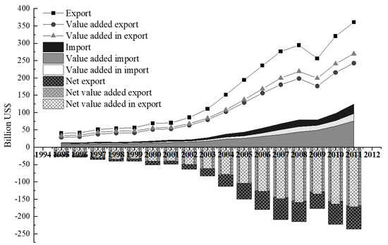
Figure 1.
China–US trade under three accounting methods (The data required for the calculations are from WOID 2013).
According to the gross trade accounting method, China’s exports of goods to the United States were $361 billion, imports were $124 billion and net exports were $236 billion US dollars in 2011. Based on the value-added-in trade accounting, the actual domestic value added of China’s exports to the United States was $270 billion, the domestic value added of US exports to China was $97 billion, and the net domestic value added in exports was $173 billion.
The trade balance in value-added trade was 37% lower compared to the gross trade. According to value-added trade statistics, China’s exports to the United States were $243 billion, imports were $76 billion and net exports were $167 billion in 2011. Compared with gross trade, the trade balance was 42% lower. The gross trade statistics seriously overestimated China’s trade surplus with the US. From 1995 to 2011, compared with the other two accounting frameworks, the trade balances under gross trade statistics were 35% and 40% higher, respectively.
The export, import and net import values based on the gross trade accounting method were the largest, and the corresponding values calculated by value-added trade and value-added-in trade accounting methods were smaller. These results consistently point to the distortion of economic benefits by the current gross trade statistics and the exaggeration of the benefits gained by China. As mentioned earlier, the “double count” problem caused by intermediate goods trade and the unclear sources of the value of the goods lead to the inaccuracy of gross trade statistics.
There are discrepancies between the real contribution in trade and traditional trade statistics [1,2]. Value added in trade is a decomposition of gross trade proposed to deal with the above problems. According to the definition in the KWW framework, value added exports based on value-added-in trade excluded foreign value added, returned domestic value added and pure double counting parts. It makes sense that value added export based on value-added-in trade is smaller than the export in gross trade.
Regardless of the methods, China gained trade surplus in the Sino–US trade in goods. China has indeed gained considerable economic benefits in its trade with the United States, but it should be recognized that gross trade statistics do indeed overestimate the current trade surplus.
Figure 2 shows the changes in the proportion of DVA in bilateral trade over the period from 1995–2011. The proportion of domestic value added exports between China and the United States experienced a process of rising, falling, rising and falling. Specifically, the proportion of domestic value added in bilateral goods trade exports peaked in 1998 (85% in China and 84% in the United States) and then began to decline. China reached the bottom of 71% in 2005, and the United States reached the bottom in 2006. After that, China rebounded but started to decline again after 2009.
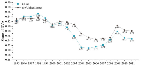
Figure 2.
The proportion of DVA in Sino–US trade in goods from 1995 to 2011 (The data required for the calculations are from WOID 2013).
At first, the proportion of DVA in China’s exports was higher than that in the United States, but this reversed after 2000. As of 2011, China’s DVA accounted for 75% and the United States 78%. This may be due to the enhancement of China’s integration into the global value chain. Compared with the United States, China engaged in lower-end and lower-profit production processes. The average share of DVA in China’s exports to the United States was 78%, and the counterpart share of the US was 80%. This further proves that China’s profitability in bilateral trade is lower than that of the United States.
Figure 3 shows the exports, imports and net exports by industry between China and the United States in 2011. Regardless of the accounting methods, most industries in China maintained a surplus in the trade of goods with the United States.
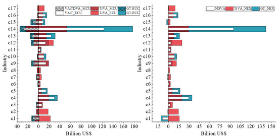
Figure 3.
Import, export and net export of Sino–US trade by industry under different accounting methods in 2011 (The data required for the calculations are from WOID 2013).
Comparing the three accounting methods, the gross trade framework underestimated the exports of China’s primary industries (c1 and c2) in 2011. Under the caliber of value-added trade, primary industries changed from deficit to surplus. The reason may be that c1 and c2 are primary products and resource products, which are used as intermediate products into the production process of other industries. Products may be indirectly exported to the United States through other countries.
On the contrary, the gross trade flow greatly overestimated the exports of China’s secondary industry (c3 c17) . Among the 15 industries, there are eight industries where the exports are overestimated and the exports based on gross trade are overestimated by an average of 151% compared to the value-added trade, while the remaining seven industries are underestimated, with an average of 35% underestimated. Among them, the leather and leather and footwear (c5), the machinery and nec (c13) and the electrical and optical equipment (c14) were overestimated by 201%, 108% and 233%, respectively.
This may be due to c13 and c14 having a relatively high degree of vertical specialization. Exports of these industries contain a large number of other countries’ content, and their products have repeatedly crossed borders resulting in the double counting problem, which, in turn, exaggerates the actual export volume. In addition, c5, c13 and c14 are final consumer industries, and their production requires a large amount of intermediate input from other industries.
Thus, imports and exports measured by value-added trade are smaller than the imports and exports calculated in gross trade. Pulp, paper, paper and printing and publishing (c7) were underestimated by 57%, coke, refined petroleum and nuclear fuel (c8) were underestimated by 68%, and the electricity, gas and water supply (c17) were underestimated by 98%. Exports from these industries are undervalued because their products are often produced as intermediate inputs to other industries.
Overall, the profitability of the primary industry was underestimated by 94%, while the profitability of the secondary industry was overvalued by 77%. The economic benefits of the primary industry were underestimated, but due to the smaller output of the primary industry, taking the country as a whole, the trade volume based on gross trade terms was still overestimated by 49% compared to that of value-added trade. With the exception of mining and quarrying (c2), coke, refined petroleum and nuclear fuel (c8) and the production and electricity, gas and water supply (c17), the remainder of US exports of goods to China are overvalued.
Compared to value-added trade, US primary industry exports to China were overvalued by 39%, US secondary industry exports to China were overvalued by 73%, and exports of goods trade were overvalued by 64%. China’s net exports of goods to the United States based on gross trade were overestimated by 41%. From the point of view of net exports, the primary industry was underestimated by 140%, and the secondary industry was overestimated by 82%. Overall, it was overrated by 42%.
Figure 4 show the source of value at the industry level of bilateral trade in goods between China and the United States. On the whole, DVA accounted for 75% of China’s exports of goods to the United States in 2011, MVA accounted for 2%, OVA accounted for 19%, RDV accounted for 1%, and PDC accounted for 3%. DVA accounted for 78% of US exports to China, MVA accounted for 2%, OVA accounted for 11%, RDV accounted for 5%, and PDC accounted for 5%.
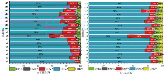
Figure 4.
Value sources in China–US bilateral trade at country level in 2011 (The data required for the calculations are from WOID 2013).
The DVA in China’s exports is generally lower than that of the United States, indicating that China’s export profitability was lower. In addition, FVA was larger in most sectors of China compared with those of the United States, except for the agriculture, hunting, forestry and fishing (c1), food, beverages and tobacco (c3), textiles and textile products (c4), leather, leather and footwear (c5), coke, refined petroleum and nuclear fuel (c8) and transport equipment (c15). A plausible reason could be compared with the United States, these industries in China are less embedded in the global value chain, and the intermediate inputs of other countries are less used.
In addition, coke, refined petroleum and nuclear fuel (c8) accounted for the lowest proportion of DVA in both China and the United States, indicating that this industry has a relatively high degree of vertical specialization, and its products were used as intermediate products in many countries.
4.2. Embodied Pollution in Sino–US Trade
Figure 5 shows the export, import and net export of SO and NO embodied by Sino–US bilateral trade in goods under three different accounting models. From 1995 to 2002, the embodied pollution exports declined slightly in fluctuations. After joining the World Trade Organization (WTO) in 2002, the embodied pollution exports increased rapidly and then declined after 2006 and 2008. The years 2002 and 2008 coincided with the time of China’s accession to the World Trade Organization and the financial crisis. This is not entirely consistent with the trend of rising exports. Especially after 2006 and 2007, the embodied pollution exports decreased, while exports increased. This may indicate the effectiveness of China’s environmental regulations, the promotion of cleaner production technologies and the changes in the structure of export commodities.
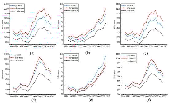
Figure 5.
The embodied SO and NO in Sino–US bilateral trade under the three accounting methods (The data required for the calculations are from WOID 2013) (a–f).
Comparing the results of the three accounting methods, we found that, unlike the results of economic benefit accounting, the export of embodied pollution based on the value-added trade framework exceeds that of the gross trade. In other words, the gross trade statistics overestimate China’s exports to the United States but underestimate China’s environmental pollution emissions caused by the exports to the United States.
Specifically, according to gross trade framework, embodied SO and NO in China’s exports to US from 1995 to 2002 averaged 1062 kilotons and 467 kilotons, and, after 2002, embodied pollutants exports climbed rapidly until they peaked in 2008 and 2006, reaching 1884 and 946 kilotons, respectively, an increase of 63% and 118% compared to 1995 and fell back to 1516 kilotons in 2011. According to value-added trade terms, from 1995 to 2002, embodied SO and NO exports averaged 1199 and 463 kilotons, with peaks of 2217 and 1034 kilotons, respectively. Compared with 1995, SO and NO exports increased by 77% and 146%, and their exports fell to 1793 and 745 kilotons in 2011. Compared with the value-added trade, the embodied pollution exports based on gross trade from 1995 to 2011 underestimated the pollution emissions by 14% and 4%, respectively.
Except for individual years, the embodied pollution imports were all on the rise, but the total amount was small compared to that of export. According to the gross trade, embodied SO and NO imports rose from 35 and 38 kilotons in 1995 to 87 and 105 kilotons in 2011, an increase of 149% and 173%, respectively. According to the value-added trade framework, the embodied SO and NO imports increased from 38 and 34 kilotons in 1995 to 99 and 90 kilotons in 2011, an increase of 158% and 165%, respectively. Although imports of Sino–US bilateral trade in goods have grown rapidly, the total volume was still small.
Regardless of the accounting method, China has always been a net exporter of pollution. While reaping economic benefits, China has also paid huge environmental costs. On average, embodied SO and NO net exports based on gross trade are underestimated by 14% and 5% comparing to value-added trade. The embodied pollution exports, imports and net export based on the value-added-in trade are the smallest. From 1995 to 2011, the embodied SO and NO based on value-added-in trade in China’s exports of goods to the United States accounted for 79% and 79% of emissions based on gross trade, while the share of correspondent emissions in US exports to China were 78% and 80%, respectively.
Figure 6 shows the embodied SO and NO in exports, imports and net exports by industry in 2011 under different accounting frameworks. Regardless of the accounting framework, most industries in China were pollution net exporters, indicating that China has paid heavy environmental costs for economic benefits. By comparing the results of different accounting methods, the following conclusions can be drawn.
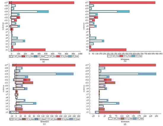
Figure 6.
The embodied SO and NO in Sino–US bilateral trade by industry in 2011 (The data required for the calculations are from WOID 2013) (a–d).
From the perspective of exports, pollution exports based on value-added trade were more concentrated, while pollution exports according to gross trade were more scattered. According to the gross trade framework, the embodied SO in China’s exports of goods to the United States are mainly concentrated in the electrical and optical equipment (c14) and textiles and textile products (c4), accounting for 36% and 13%, respectively. The embodied SO based on value-added trade are mainly concentrated in the electricity, gas and water supply (c17) and agriculture, hunting, forestry and fishing (c1), and these two industries accounted for 51% and 28%, respectively, together accounting for 78% of total embodied pollution export.
As with the situation of SO, the embodied NO in China’s exports to the United States based on gross trade in 2011 are also mainly concentrated in the electrical and optical equipment (c14) and textiles and textile products (c4), together accounting for 49%. The embodied NO based on the value-added trade are mainly concentrated in the electricity, gas and water supply (c17) and agriculture, hunting, forestry and fishing (c1), accounting for 36% and 27%, respectively, together accounting for 63%. The major pollution emission industries also changed.
In China’s exports of goods to the United States, the top two embodied SO and NO emission industries changed from electrical and optical equipment (c14) and textiles and textile products (c4) to electricity, gas and water supply (c17) and agriculture, hunting, forestry and fishing (c1).
From the perspective of imports, embodied pollution based on value-added trade was more concentrated, and the major pollution emission industries changed. This is similar to the export situation. According to the gross trade terms, the embodied SO in the United States’ exports of goods to China were mainly concentrated in c chemicals and chemical products (c9) and basic metals and fabricated metal (c12), accounting for 29% and 18%, respectively.
The embodied SO based on value-added trade were mainly concentrated in the electricity, gas and water supply (c17) and chemicals and chemical products (c9), and these two industries together accounted for 59% of the total imports. According to gross trade statistics, the embodied NO imports from the United States in 2011 were also mainly concentrated in agriculture, hunting, forestry and fishing (c1) and chemicals and chemical products (c9), accounting for 28% and 14%, respectively, and together accounting for 42% in total.
The embodied NO emissions based on value-added trade were mainly concentrated in electricity, gas and water supply (c17) and agriculture, hunting, forestry and fishing (c1), accounting for 26% and 20%, respectively, and accounted for 46% in total. At the same time, the top two embodied SO import industries changed from the electrical and optical equipment (c14) and textiles and textile products (c4) to the electricity, gas and water supply (c17) and agriculture, hunting, forestry and fishing (c1). The top two embodied NO import industries changed from the electrical and optical equipment (c14) and textiles and textile products (c4) to the electricity, gas and water supply (c17) and agriculture, hunting, forestry and fishing (c1).
It seems that different accounting frameworks lead to different results at industry level. A plausible explanation may be that the gross trade flow is calculated on the basis of the total output, and the value-added trade is calculated on the basis of the forward link as are pollution emissions. Pollution emissions of value added exports include not only the emission of this sector, but also the emission of indirect exports through other sectors. Industries, such as the electrical and optical equipment (c14) and the textiles and textile products (c4), may have a large output. However, since their total output actually includes intermediate inputs from other industries, their economic benefits and corresponding pollution emission calculated in gross terms may be exaggerated. Industries, such as the electricity, gas and water supply (c17) are often served as intermediate inputs for other industries. A large part of their exports (pollution emission) is indirectly exported through other industries and is not included in the total exports of the industry itself.
4.3. Estimating China’s Economic-Environmental Status in Bilateral Trade
Figure 7 shows PIE, PIM and PTT in bilateral trade from 1995 to 2011. Regardless of the accounting framework, China’s PIE is higher than that of the United States, which indicates that China’s pollution emissions for per unit of value-added exports were greater than those caused by US exports. The reason could be that the production in the United States is cleaner, or that China’s environmental regulation was looser than the United States. PIE and PIM have basically maintained a downward trend in the period, indicating that the pollutants contained in each unit of value-added exports of both countries are decreasing, and the production of both countries is becoming cleaner.
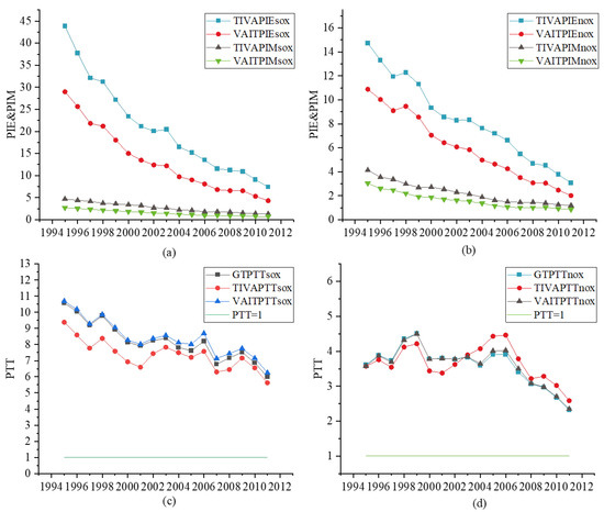
Figure 7.
PIE, PIM and PTT of SO and NO in Sino–US bilateral trade (The data required for the calculations are from WOID 2013) (a–d).
The PIE based on value-added trade is larger than that based on value-added-in trade. In other words, using the value-added-in-trade method will underestimate the pollution contained in China’s exports for per unit of value added, and this conclusion holds for both pollutants. On average, PIE of SO and NO calculated based on value-added-in trade was underestimated by 36% and 28%. For US exports to China, the conclusions are similar. On average, the PIE of SO and NO calculated based on the value-added-in trade framework was underestimated by 45% and 28%.
Regardless of the accounting frameworks, China’s PTT relative to the United States was far greater than 1, indicating that China has paid a greater environmental cost for the same amount of economic benefits. From 1995 to 2011, PTT showed a fluctuating and declining trend, meaning that, considering both economic benefits and environmental pollution, China is at a disadvantage, but the situation is constantly improving. Before 2003, according to gross trade statistics, PTT of SO and NO dropped from 11 and 3 in 1995 to 6 and 2 in 2011; according to value-added-trade statistics, PTT of SO and NO dropped from 9 and 4 in 1995 to 6 and 3 in 2011; according to value added statistics, PTT of SO and NO fell from 11 and 4 in 1995 to 6 and 2 in 2011.
The trend of the PTT calculated by the gross trade and value-added-in trade framework is consistent, and their values are very close. The differences between the PTT of SO and NO were 0.21 and 0.03 on average, respectively. For SO, PTT based on value-added-in trade was the highest, followed by that of gross trade and value-added trade. On average, PTT based on gross trade was 11% overestimated compared to that of value-added trade and was underestimated by 2% compared to that of value-added-in trade. For NO, PTT based on gross trade and value-added-in trade were lower than those of value-added trade before 2003. After 2003, PTT based on value-added trade was higher.
Figure 8 shows the PTT of SO and NO by industry under gross trade statistics and value-added trade from 1995 to 2011. It can be proven that the calculation results of the industry-level PTT based on gross trade and that of value-added-in trade are equal, but the conclusion does not hold at the national level. The mathematical proof is shown in Appendix B. In the bilateral trade of goods between China and the United States, most industries in China are also at a disadvantage (PTT > 1).
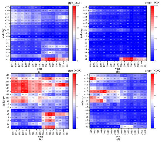
Figure 8.
The PTT index of SO and NO in Sino–US bilateral trade (The data required for the calculations are from WOID 2013) (a–d).
The PTT of most industries is improving, and some industries deteriorated first and then improved. Compared with 1995, only the PTT of the agriculture, hunting, forestry and fishing (c1) increased, that is, the PTT in 2011 worsened compared with 1995. In addition, the PTT of the agriculture, hunting, forestry and fishing (c1) were very high. In 2011, the PTT of SO were 23 based on the gross trade statistics, and, under the value-added-trade statistics, the pollution terms of trade even reached 78. The turning point came in 2004.
A plausible explanation is the vigorous promotion of agricultural mechanization in China. The "Law of the People’s Republic of China on the Promotion of Agricultural Mechanization" was promulgated in 2004. Since then, seven consecutive No. 1 documents from the central government have been promulgated, constantly emphasizing the support for agricultural mechanization.
During the Eleventh Five-Year Plan period , the central government’s total investment in subsidies for purchasing machines reached 35.1 billion yuan. Agricultural machinery and equipment burn a large amount of diesel fuel, which, in turn, generates gas pollution. This may explain the sudden deterioration of PTT in the agricultural sector in 2004. In general, gross trade statistics overestimate the PTT.
5. Conclusions
In this paper, we used the input–output data in the WIOD database from 1995 to 2011 to calculate the economic benefits and embodied pollution in Sino–US bilateral trade and used three different accounting frameworks to measure and calculate other related indicators and observe the influences of different methods on the results. The main conclusions are as follows:
No matter what accounting method is used, the conclusion that China has maintained a long-term surplus in Sino–US trade in goods has not changed. Comparing the economic benefits under three accounting frameworks at the national level, it can be found that the export, import and net import values based on the gross trade were the largest, while those based on the value-added trade and value-added-in trade values were smaller. Using KWW to decompose the gross trade flow between China and the United States, we found that, after 2000, the proportion of DVA in China’s exports is lower than that of the United States, indicating that China’s profitability is lower than that of the United States.
Gross trade statistics clearly underestimated China’s exports to the United States from the primary industry in 2011. Under the value-added trade framework, the two sub-industries belonging to the primary industry changed their trade deficit to a surplus. In contrast, the gross trade statistics greatly overestimated China’s secondary industry exports. This may be related to the role of industry products in production—as an intermediate input into the production process of other industries or more products from other industries are needed as intermediate inputs.
While maintaining a surplus in trade of good, China has been a pollution net exporter in Sino–US trade, which means that China has paid huge environmental costs in exchange for economic benefits. This is consistent with the conclusions of many scholars. Through the comparison of different accounting methods, we found that the embodied pollution of exports based on the value-added trade framework accounting exceeded that of gross trade. In other words, the total value trade statistics overestimated the economic benefits of China’s exports to the United States.
When analyzing the embodied pollution of Sino–US trade in goods at the industry level, we found that the embodied pollution under the value-added-trade statistics is more concentrated, while under gross trade statistics is more scattered, and the major pollution industries also changed. The results of industry economic benefits under gross trade statistics and value-added-trade statistics are quite different. Different accounting frameworks have a great influence on pollution emission results.
In the study interval, the pollution intensity of China’s exports to the United States was higher than that of the United States’ exports to China. This shows that China produces more pollution for obtaining a unit of value added. Fortunately, PIE and PIM maintained a downward trend, indicating that that the production of both countries is becoming cleaner. The export intensity calculated by the value-added-trade method is higher than that calculated by the value-added-in-trade method, which is consistent with the more serious pollution under the value-added-trade method.
In addition, PTT were far greater than 1 and showed a trend of declining, showing that China paid greater environmental costs for the same amount of economic benefits and though China was at a disadvantage in bilateral trade, the situation was constantly improving. At last, when analyzing at the industry level, gross trade statistics will overestimate PTT. In other words, gross trade statistics will underestimate China’s environmental protection progress.
Sino–US trade is a representative of the North–South trade, and thus some of its conclusions can be extended to other bilateral North–South trades. Based on this and the conclusions above, two policy recommendations are provided. For developing countries, such as China, embodied pollution in trade should be taken seriously. Many developing countries have concentrated on the economic benefits and attempted to improve the competitiveness and technology of products to move up the global value chain.
However, as the conclusions indicate, the environmental costs are huge. Developing countries could introduce advanced foreign production technology to improve energy efficiency, use clean energy and adopt green tax and green finance to control industrial pollution emissions. As for developed countries, like the US, the environmental benefits gained from trade should not be neglected. Developed countries should maintain their edge in profitability and technology and could provide technical service and cleaner production technology to make profits.
There are limitations in our work. We used the pollution intensity in 2009 as the proxy of that of 2010 and 2011, which implies the assumption that the intensity of pollution emissions in China and the United States remained unchanged during 2009–2011. The input–output method we used to estimate economic benefits was based on the proportionality assumption, which would result in the overestimation of value-added exports [41]. In addition, this paper focused on re-examining the economic benefits and environmental costs in Sino–US trade and compared the differences in results under different models, but we have not rigorously proved why these differences occur theoretically or in math. Such proof would be interesting and important, and this will also be a focus of our future research.
Author Contributions
L.-Y.H. is a full professor of economics. H.H. is a Master degree candidate supervised by L.-Y.H. Both authors contributed significantly in the project. L.-Y.H. acquired all the funding supports. H.H. calculated the results under L.-Y.H.’s supervision. L.-Y.H. and H.H. analyzed the data, discussed the results and co-wrote the manuscript. All authors have read and agreed to the published version of the manuscript.
Funding
This work was supported by the State Key Project of the National Social Science Foundation of China (Grant No. 19AZD003).
Institutional Review Board Statement
Not applicable.
Informed Consent Statement
Not applicable.
Data Availability Statement
“World Input–Output Database” at http://www.wiod.org/home accessed on 26 July 2021.
Conflicts of Interest
The authors declare no conflict of interest.
Appendix A
Based on an input–output approach, considering a world with G countries and N sectors, gross output produced in the world can be expressed as followed:
is the vector of gross output in country i. is a submatrix of technical input–output coefficients, giving units of intermediate goods produced in i used for the use of production of one unit gross output in country j. is the final demand vector, giving the final goods produced in country i and consumed in country j.
With arranging, we have:
is the Leontief inverse matrix. is a submatrix, which shows the whole demand of the output of country i for unit final products of country j.
Let refer to a diagonal direct value-added coefficient matrix and refer to value-added production matrix that gives domestic value added in countries’ gross output. can be computed as:
Appendix B
It can be proved that the calculation results of the industry-level PTT based on gross trade are consistent with those based on value-added-in trade, but the conclusion does not hold at the national level. The mathematical proof is as follows:
When calculating at the industry level, because there is no need to add up, the vector calculation is directly used to calculate the industry’s PTT.
; ; ; .
;
When calculating at the national level, the two are not equal due to the totalization involved.
;
References
- Feenstra, R.C. New Evidence on the Gains from Trade. Rev. World Econ. 2006, 142, 617–641. [Google Scholar] [CrossRef]
- Koopman, R.; Powers, W.M.; Wang, W.; Wei, S.J. Give Credit Where Credit is Due: Tracing Value Added in Global Production Chains; National Bureau of Economic Research: Cambridge, MA, USA, 2010. [Google Scholar]
- Schmalensee, R.; Stoker, T.M.; Judson, R.A. World carbon dioxide emissions: 1950–2050. Rev. Econ. Stat. 1998, 80, 15–27. [Google Scholar] [CrossRef]
- Galeotti, M.; Lanza, A. Richer and cleaner? A study on carbon dioxide emissions in developing countries. Energy Policy 1999, 27, 565–573. [Google Scholar] [CrossRef] [Green Version]
- Lin, J.; Pan, D.; Davis, S.J.; Zhang, Q.; He, K.; Wang, C.; Streets, D.G.; Wuebblesg, D.J.; Guan, D. China’s international trade and air pollution in the United States. Proc. Natl. Acad. Sci. USA 2014, 111, 1736–1741. [Google Scholar] [CrossRef] [PubMed] [Green Version]
- Guan, D.; Su, X.; Zhang, Q.; Peters, G.P.; Liu, Z.; Lei, Y.; He, K. The title of the cited article. Socioecon. Drivers China’s Prim. PM2.5 Emiss. 2014, 9, 1–9. [Google Scholar]
- Genty, A.; Arto, I.; Neuwahl, F. Final database of environmental satellite accounts: Technical report on their compilation. WIOD Deliv. 2012, 4. [Google Scholar]
- Lenzen, M.; Murray, J.; Sack, F.; Wiedmann, T. Shared producer and consumer responsibility—Theory and practice. Ecol. Econ. 2007, 61, 27–42. [Google Scholar] [CrossRef]
- Zhang, B.; Bai, S.; Ning, Y.; Ding, T.; Zhang, Y. Emission Embodied in International Trade and Its Responsibility from the Perspective of Global Value Chain: Progress, Trends, and Challenges. Sustainability 2020, 12, 3097. [Google Scholar] [CrossRef] [Green Version]
- Antweiler, W. The pollution terms of trade. Econ. Syst. Res. 1996, 8, 361–366. [Google Scholar] [CrossRef]
- Duan, Y.; Yan, B. Economic gains and environmental losses from international trade: A decomposition of pollution intensity in China’s value-added trade. Energy Econ. 2019, 83, 540–554. [Google Scholar] [CrossRef]
- Xiong, Y.; Wu, S. Real economic benefits and environmental costs accounting of China–US trade. J. Environ. Manag. 2020, 279, 111390. [Google Scholar] [CrossRef] [PubMed]
- Varian, H.R. An iPod has global value. Ask the (many) countries that make it. New York Times 2007, 10, 28. [Google Scholar]
- Xing, Y.; Detert, N.C. How the iPhone Widens the United States Trade Deficit with the People’s Republic of China. ADBInstitute : Tokyo, Japan, 2010. [Google Scholar]
- Daudin, G.; Rifflart, C.; Schweisguth, D. Who produces for whom in the world economy? Can. J. Econ. 2011, 44, 1403–1437. [Google Scholar] [CrossRef] [Green Version]
- Johnson, R.C.; Noguera, G. Accounting for intermediates: Production sharing and trade in value added. J. Int. Econ. 2012, 86, 224–236. [Google Scholar] [CrossRef] [Green Version]
- Stehrer, R. Trade in Value Added and the Valued Added in Trade. WIIW Working Paper: Vienna, Austria, 2012. [Google Scholar]
- Koopman, R.; Wang, Z.; Wei, S.J. Tracing value-added and double counting in gross exports. Am. Econ. Rev. 2014, 104, 459–494. [Google Scholar] [CrossRef] [Green Version]
- Wang, Z.; Wei, S.; Zhu, K. Quantifying International Production Sharing at the Bilateral and Sector Levels; National Bureau of Economic Research: Cambridge, MA, USA, 2013. [Google Scholar]
- Aleksandra, K.; Olczyk, M. CEE trade in services: Value-added versus gross terms approaches. East. Eur. Econ. 2018, 56, 269–291. [Google Scholar]
- Wang, L.; Sheng, B. China–US Trade in Value-added and Gains from Bilateral Trade in Global Value Chains. J. Financ. Econ. 2014, 9, 97–108. (In Chinese) [Google Scholar]
- Liu, Z.; Meng, J.; Deng, Z.; Lu, P.; Guan, D.; Zhang, Q.; Gong, P. Embodied carbon emissions in China–US trade. Sci. China Earth Sci. 2020, 63, 1577–1586. [Google Scholar] [CrossRef]
- Dai, F.; Yang, J.; Guo, H.; Sun, H. Tracing CO2 emissions in China–US trade: A global value chain perspective. Sci. Total Environ. 2021, 775, 145701. [Google Scholar] [CrossRef]
- Wang, Q.; Zhou, Y. Uncovering embodied CO2 flows via North–North trade—A case study of US–Germany trade. Sci. Total Environ. 2019, 691, 943–959. [Google Scholar] [CrossRef] [PubMed]
- Zhang, Z.; Xi, L.; Bin, S.; Yuhuan, Z.; Song, W.; Ya, L.; Guang, S. Energy, CO2 emissions, and value added flows embodied in the international trade of the BRICS group: A comprehensive assessment. Renew. Sustain. Energy Rev. 2019, 116, 109432. [Google Scholar] [CrossRef]
- Wu, R.; Geng, Y.; Dong, H.; Fujita, T.; Tian, X. Changes of CO2 emissions embodied in China—Japan trade: Drivers and implications. J. Clean. Prod. 2008, 112, 4151–4158. [Google Scholar] [CrossRef]
- Wang, Q.; Liu, Y.; Wang, H. Determinants of net carbon emissions embodied in Sino-German trade. J. Clean. Prod. 2019, 235, 1216–1231. [Google Scholar] [CrossRef]
- Wang, Q.; Yang, X. Imbalance of carbon embodied in South–South trade: Evidence from China–India trade. Sci. Total Environ. 2020, 707, 134473. [Google Scholar] [CrossRef]
- Lin, B.; Xu, M. Does China become the “pollution heaven” in South–South trade? Evidence from Sino–Russian trade. Sci. Total Environ. 2019, 666, 964–974. [Google Scholar] [CrossRef]
- Xu, S.; Gao, C.; Li, Y.; Ma, X.; Zhou, Y.; He, Z.; Wang, S. What Influences the Cross-Border Air Pollutant Transfer in China–United States Trade: A Comparative Analysis Using the Extended IO-SDA Method. Sustainability 2019, 11, 6252. [Google Scholar] [CrossRef] [Green Version]
- Wang, F.; Li, Y.; Zhang, W.; He, P.; Jiang, L.; Cai, B.; Jiang, H. China’s trade-off between economic benefits and sulfur dioxide emissions in changing global trade. Earth’s Future 2020, 8, e2019EF001354. [Google Scholar] [CrossRef] [Green Version]
- Tao, F.; Xu, Z.; Duncan, A.A.; Xia, X.; Wu, X.; Li, J. Driving forces of energy embodied in China-EU manufacturing trade from 1995 to 2011. Resour. Conserv. Recycl. 2018, 136, 324–334. [Google Scholar] [CrossRef]
- Chen, W.; Kang, J.N.; Han, M.S. Global environmental inequality: Evidence from embodied land and virtual water trade. Sci. Total Environ. 2021, 783, 146992. [Google Scholar] [CrossRef]
- Grether, J.M.; Mathys, N.A. The pollution terms of trade and its five components. J. Dev. Econ. 2013, 100, 19–31. [Google Scholar] [CrossRef]
- Su, B.; Ang, B.W. Multiplicative structural decomposition analysis of aggregate embodied energy and emission intensities. Energy Econ. 2017, 65, 137–147. [Google Scholar] [CrossRef]
- Meng, B.; Peters, G.P.; Wang, Z.; Li, M.T. Tracing CO2 emissions in global value chains. Energy Econ. 2018, 73, 24–42. [Google Scholar] [CrossRef] [Green Version]
- Zhang, D.; Caron, J.; Winchester, N. Sectoral Aggregation Error in the Accounting of Energy and Emissions Embodied in Trade and Consumption. J. Ind. Ecol. 2019, 23, 402–411. [Google Scholar] [CrossRef] [Green Version]
- Xu, S.C.; Gao, C.; Miao, Y.M.; Shen, W.X.; Long, R.Y.; Chen, H.; Wang, S.X. Calculation and decomposition of China’s embodied air pollutants in Sino–US trade. J. Clean. Prod. 2019, 219, 978–994. [Google Scholar] [CrossRef]
- Kim, T.J.; Tromp, N. Carbon emissions embodied in China–Brazil trade: Trends and driving factors. J. Clean. Prod. 2021, 293, 126206. [Google Scholar] [CrossRef]
- Timmer, M.P.; Dietzenbacher, E.; Los, B.; Stehrer, R.; De Vries, G.J. An illustrated user guide to the world input–output database: The case of global automotive production. Rev. Int. Econ. 2015, 23, 575–605. [Google Scholar] [CrossRef]
- Patunru, A.A.; Prema-chandra, A. Measuring trade in value added: How valid is the proportionality assumption? Econ. Syst. Res. 2021, 9, 1–9. [Google Scholar] [CrossRef]
Publisher’s Note: MDPI stays neutral with regard to jurisdictional claims in published maps and institutional affiliations. |
© 2021 by the authors. Licensee MDPI, Basel, Switzerland. This article is an open access article distributed under the terms and conditions of the Creative Commons Attribution (CC BY) license (https://creativecommons.org/licenses/by/4.0/).