Abstract
To meet power quality requirements, it is necessary to classify and identify the power quality of the power grid connected with renewable energy generation. S-transform (ST) is an effective method to analyze power quality in time and frequency domains. ST is widely used to detect and classify various kinds of non-stationary power quality disturbances. However, the long taper and scaling criteria of the Gaussian window in standard ST (SST) will lead to poor time domain resolution at low frequency and poor frequency resolution at high frequency. To solve the discrete side effects, it is necessary to select the optimal window function to locate the time frequency accurately. This paper proposes a modified ST (MST) method. In this method, an improved window function of energy concentration in time-frequency distribution is introduced to optimize the shape of each window function. This method determines the parameters of Gaussian window to maximize the product of energy concentration in a time-frequency domain within a given time and frequency interval, so as to improve the energy concentration. The result shows that compared with the SST with Gaussian window, ST based on the optimally concentrated window proposed in this paper has better energy concentration in time-frequency distribution.
1. Introduction
In order to cope with the increasingly severe energy shortages and the challenge of energy conservation and emissions reduction, the penetration rate of renewable energy generation such as photovoltaic power generation and wind power generation is increasing in power systems [1]. Renewable energy generation units connect with the power grid through power electronic equipment. However, a lot of power electronic equipment generate harmonic and reactive current in the power grid, resulting in a series of interference problems in the power system such as voltage surge, voltage sag, harmonic, short-time outage, pulse transient disturbance, high-frequency oscillation disturbance and voltage flicker [2]. Taking a photovoltaic inverter as an example, the harmonic current mainly consists of two parts [3]: (1) low-order harmonics caused by dead time, such as 3, 5, 7 odd harmonic currents; (2) high-order harmonics caused by PWM modulation process. High-frequency harmonics can be filtered by L-type or LCL type output filters [4]; for low order harmonics, parallel tuned filters are used for harmonic suppression and reactive power compensation [5]. Power quality (PQ) also has a significant impact on the safety of users, the equipment service life and power system safety. For industrial users, the PQ problems in any link may affect the final quality of products, and the PQ has a crucial impact on the quality of terminal products in modern aerospace and microelectronic industries. For residential users, the change of lighting brightness caused by voltage flicker will also cause discomfort. For power system safety, the harmonic, subharmonic and interharmonic components in the current will cause neutral point overload, transformer overheating, circuit breaker false tripping and other problems, which will cause serious consequences. Therefore, it is important to study the disturbance, identification, classification and governance of power system PQ.
The randomness of PQ disturbances makes it difficult to extract the effective feature information of PQ disturbances directly. Therefore, it is necessary to identify PQ disturbance more intelligently. In recent years, a variety of signal analysis methods have been widely used in PQ signal analysis, such as Fourier transform (FT) [6,7], wavelet transform (WT) [8,9], Hilbert-Huang transform (HHT) [10,11], short-time Fourier transform (STFT) [12], Stockwell transform (ST) [13,14,15], and so on. FT cannot determine the time distribution of frequency components of non-stationary signals. The representation of time-frequency information of PQ provides a way to solve the non-stationary characteristics. STFT applies a sliding window to analyze signal and obtain the TF spectrum by taking FT of the windowed signal. Due to the fixed time interval, STFT is difficult to use to provide a satisfactory time-frequency representation for non-stationary signals [11]. To overcome the shortcomings of STFT, WT is proposed. WT with a time-frequency window has good time and frequency resolution in both high and low frequency. However, it is difficult to select the appropriate fundamental and it is sensitive to noise [8]. The studies of Chakraborty and Okaya [16] show that continuous WT (CWT) is a good spectral interpretation method. Discrete WT (DWT) extracted components cover a wider frequency and provide better time-frequency interval flexibility. However, it lacks the ability to resist noise, especially when the signal is contaminated. In reference [17], an automatic PQ event recognition method based on HHT is proposed.
The main goal of time-frequency distribution function is to obtain the ideal time-frequency representation and the time-varying spectral density function with high resolution, and to overcome the existence of time-frequency interference. Therefore, time-frequency domain energy concentration is very important in time-frequency analysis [18,19]. The WT multi-resolution analysis method can effectively extract the disturbance characteristics of non-stationary signals, but it is easily affected by noise interference and has a large amount of calculation. It is difficult to select an appropriate wavelet basis function and to realize the disturbance signals mainly characterized by time-domain characteristics, such as voltage surge and voltage drop. The signal processing method based on sliding discrete Fourier transform [20], empirical mode decomposition, adaptive short time Fourier transform [21], wavelet packet transform [22] and filter bank method [23] are proposed to analyze non-stationary signals in various fields. These methods follow the change of time local spectrum to extract the characteristic change of non-stationary signal. In recent research, WT is widely used in power signal analysis and PQ evaluation, but WT has a local phase reference. Another powerful time-frequency analysis technique is ST. Because of its ability to predict time-domain Fourier spectrum and global phase reference characteristics, it has been widely used in PQ research [24]. In [25,26,27,28], many attempts to generalize and calculate ST faster are proposed. ST has progressive resolution, while retaining the absolute reference phase information similar to STFT [29], and has the characteristics of frequency invariant amplitude response. ST can be used as both an analysis tool and synthesis tool, which makes ST widely used in many scientific fields, including PQ signal analysis, optics, mechanical systems, pattern recognition and so on.
Window width is the main factor affecting the resolution. Narrow windows at higher frequencies and wide windows at lower frequencies result in unnecessary deterioration of time resolution and frequency resolution at lower and higher frequencies, which results in a very poor energy concentration in the time-frequency distribution. The energy concentration of ST limits its accuracy. Due to its relatively fixed Gaussian window, standard ST cannot provide satisfactory time-frequency resolution for all types of jamming signals [30]. In order to improve the time-frequency resolution and the energy concentration of time-frequency distribution, many researchers try to modify the Gaussian window function structure by introducing adjustable parameters to control the window width [31] and to optimize these parameters. Frequency-based optimization methods have been proposed to determine these parameters according to the energy concentration of signals that may be seriously disturbed under a low signal-to-noise ratio, resulting in the instability of the optimal parameters [32]. A modified ST (MST) with two parameters is proposed to control the window width, and three optimization criteria are defined to adaptively determine the parameters in reference [27]. A method based on the MST and parallel stacked sparse auto-encoder to PQ disturbances recognition is proposed in reference [33], and a Kaiser window is used in MST for a better energy concentration in time-frequency matrix. Since adaptive time-frequency resolution is not the best time-frequency resolution for feature extraction, there are certain limitations in time-frequency extraction for different characteristic signals. As mentioned above, the time-frequency analysis algorithm extracts information from PQ interference signals, and the energy concentration directly affects the accuracy of features. The appropriate window function can be chosen according to the analysis signal. In this paper, a modified ST method for obtaining optimal energy concentration by time-frequency domain analysis is proposed based on standard S-transform. The MST method can maximize the energy concentration by adjusting the additional parameters of Gaussian window in a finite time and frequency range.
The remainder of the paper is organized as follows: Section 2 presents the model of the standard S-transform. Then, a modified ST method for obtaining optimal energy concentration by time-frequency domain analysis is proposed in Section 3. In Section 4, the validity of the proposed method is verified by experiments. Finally, a conclusion is presented in Section 5.
2. Standard S-Transform
S-transform was first proposed by Stockwell in 1996 and it is a time-frequency analysis method originated from STFT. ST can also be derived from WT, which has the characteristics of multi-resolution. ST preserves the phase information of signal in STFT and provides the variable resolution of WT.
The WT of x(t) is defined [13] as follows, and the one-dimensional continuous signal .
where is the basis function of WT; is the scale factor of WT.
When a Gaussian window function is selected as the basis function of WT, the corresponding WT is
In general, the Gaussian window function directly affects the time-frequency resolution of ST and it can be defined as [13]
where τ is the time shift factor; σ is the frequency expansion factor, as follows
Multiply the right side of Equation (2) by the phase correction factor, and modify the amplitude of , substitute . Therefore, the ST is obtained by
Furthermore, the Gaussian window can be extended to
where is the standard deviation of the Gaussian window, which depends on the frequency and parameter set {P}.
ST can be used to analyze the amplitude, frequency and phase of the signal simultaneously. The Gaussian function is widely used in signal processing, and the product of frequency and time resolution can be minimized by using the Gaussian function. In (3), the width of the window is inversely proportional to the frequency f, which makes the window width wide at low frequency and narrow at high frequency. Therefore, ST achieves high-frequency resolution at low frequency and high time resolution at high frequency [34].
The window function provides better frequency domain location for low frequency and time domain location for high frequency [27]. The ST method has been widely used in time-frequency analysis of signal, but there are still limitations in energy concentration. The energy concentration is improved by adjusting the parameters of the Gaussian window, but the uncertain parameter adjustment standard is left. According to the Heisenberg Gabor limit, it is difficult to balance the accuracy in time domain and frequency domain.
In a discrete case, a discrete signal x[kT] (k = 0, 1, 2, …, N − 1), N denotes total sampling points, T represents the sampling period. The discrete FT of h[kT] is defined as [13,28]
where n = 0, 1, 2, …, N − 1.
When τ = kT and f = n/NT, the discrete ST is calculated as follows
where . When , it can be represented as
The discrete ST directly uses discrete and truncated form of the Gaussian window in frequency domain, which is expressed as
where represents the standard deviation of the Gaussian window in a time domain, and the corresponding frequency domain term is .
3. S-Transform Based on Optimally Concentrated Window
3.1. Modified S-Transform
It can be clearly seen from Equations (3) and (4) that the window width always changes with the reciprocal of frequency f. Because the time-frequency resolution of ST is determined by a relatively fixed window, the time-frequency resolution of various signals remains unchanged. Time-frequency resolution should be controlled to adapt to different signals in application. The Heisenberg uncertainty principle points out that the time and frequency resolution of signal cannot be improved together [35].
In the process of frequency feature extraction of disturbance signal, although the Gaussian window width of ST can be adjusted, the adaptability of adjustment range is general, and the energy concentration measure is not enough. To maximize the energy concentration of Gaussian window for the desired signal to be measured, adjustable factors a, b, c and d are introduced into ST. Therefore, the modified S-transform is based on optimally concentrated window, shown as Equation (11).
The Gaussian window function is generalized and three new parameters are introduced. The standard deviation of the window is modified to
The generalized Gaussian window function in frequency domain can be expressed as
where a is the parameter that controls the trade-off between STFT and ST, b defines the way of window width change, c is the parameter that defines the change rate of window width, and d is the window width factor. If and only if , , and , MST will be the standard ST; if , , and , the form of MST is STFT. When or , the time resolution of signal increases and the frequency resolution decreases; when or , the frequency resolution of the signal increases and the time resolution decreases.
MST shown in Equations (11) and (12) can also be written as a function of H(f)
In a discrete case, the MST of the discrete domain can be expressed as
where n is the index of each time sample and N is the total number of samples or signal length. The window factor is
where t = nT, f = v/NT. T is the exponential frequency sample of sampling time.
3.2. Adaptation of the Generalised Window Parameters
In the process of determining the auxiliary parameters a, b, c and d of MST, the maximum value of ECM is expected. The rate of change of energy is expressed as
where t = nT, f = v/NT. T is the exponential frequency sample of sampling time.
The expression of measured signal ECM is as follows:
Taking the maximum energy concentration as the performance index, the appropriate window parameters are selected. The optimal value of the window parameters of the generalized window is obtained by
The width of the window is inversely proportional to the frequency f, which makes the window wide at low frequency and narrow at high frequency. Therefore, the time resolution will be low if the width of the Gaussian window is too narrow; and the frequency resolution will be too poor if the width of the Gaussian window is too wide.
is selected to be 4 by the sampling frequency; is determined by the number of dominant frequencies of the signal to obtain the better frequency resolution. The minimum frequency of signal fmin is 1 Hz, and the maximum frequency of signal fmax is decided by itself.
The nonlinear constraint problem expressed by Equations (16), (21) and (22) is solved, and the appropriate Gaussian window is selected. Therefore, the shape of the window varies adaptively for each analysis frequency to obtain an accurate time-frequency distribution with higher energy concentration. Optimization can be carried out by time or frequency variables.
3.3. Algorithm
Based on the above, a parameter optimal variational scheme based on frequency is given below. This can be considered as a nonlinear optimization problem with constraints. An active-set strategy is applied [36]. The scheme provides us with the frequency conversion parameter and applies it to the deformation correction. Therefore, the algorithm of can be summarized by the following steps, and the algorithm flow chart is shown in Figure 1.
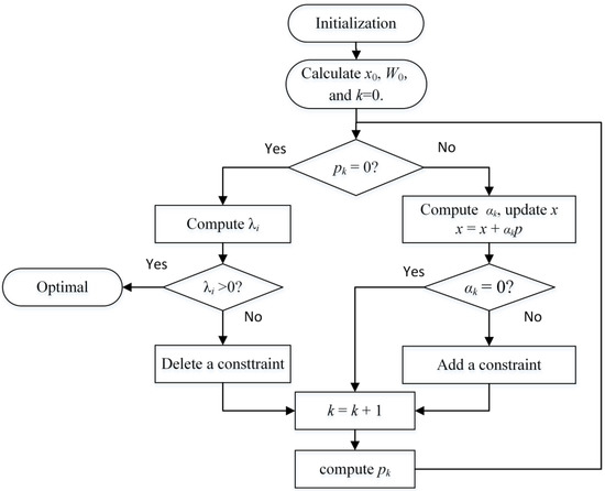
Figure 1.
Algorithm flow chart of active-set method.
Suppose that the initial iteration point is , and the initial working set is
.
- Calculate the feasible initial point , and the efficient constraint set at is . ;
- Solve the subproblem, and get ;
- If , calculate the corresponding value of that meets the requirements, and ;If , the calculation is stopped, and . Otherwise, select to make meet the requirements. Let , , then turn to step 5;
- If , calculate the value of ; if , calculate the values of to make meet the requirements, and let . Then turn to step 5;
- , and turn to step 2.
The optimization window of MST at the fundamental frequency is narrower than that of ST, which can obtain higher time resolution, and is suitable for the location of voltage sag and voltage swell. In the high-frequency band, the Gaussian window of MST is wider than that of ST; therefore, MST has better frequency resolution, which is suitable for feature extraction of high-order harmonics, transient oscillation and other analysis objects.
4. Simulation Results and Discussion
The power quality disturbance signal has many styles and features. In order to improve the energy concentration of the signal, adjustable factors a, b, c and d are introduced into ST. The introduced parameters (a, b, c and d) control the shape of the window and they are chosen as follows: 0 ≤ a, b, c and d ≤ 3. We apply the proposed S-transform on the analysis of power quality disturbance signals and we compare its energy concentration with standard S-transform.
We propose to compare with four classes of synthetic signals, i.e., signals with sinusoidal-modulated components. Four kinds of power quality disturbance signals, including voltage sag and voltage swell, transient oscillation, voltage interruption and voltage sag with harmonics, are selected as simulation signals in this experiment. Matlab R2016a is used to simulate the signals mentioned above. The voltage amplitude A of all signal models is normalized to 1. The fundamental frequency is 50 Hz. The is the time difference between the start time and the end time of the disturbance, and T indicates the signal period.
4.1. Voltage Sag and Voltage Swell
The signals can be given as: , . The sinusoidal modulated component is added in the time period of , and the amplitude of voltage decreases first and then increases. The analysis results of S-transform and modified S-transform are shown in Figure 2b,c respectively.

Figure 2.
Analysis results of voltage sag and voltage swell. (a) The original signal of voltage sag and voltage swell. (b) The analysis results of S-transform. (c) The analysis results of modified S-transform.
Figure 2a shows the original signal. Figure 2b is the analysis result chart of standard S-transform, and Figure 2c shows the analysis result chart of modified S-transform. The abscissa in Figure 2b represents the times, and the ordinate represents the frequency standard unit value. The colors represent the per unit value of signal amplitude. As can be seen from Figure 2b, the amplitude begins to decrease at 0.01 s, and the peak appears in the high frequency band at 0.02 s, indicating that the amplitude decreases. At 0.13 s, the peak appears again in the high-frequency band, and the amplitude begins to increase at 0.14 s, indicating that the amplitude increases. In Figure 2c, the frequency of the signal is concentrated between 47 Hz and 52 Hz after MST, and the energy concentration is obviously higher. The change of amplitude is clearer using the MST method. As can be seen from Figure 2c, the amplitude decreases at 0.027 s and increases at 0.126 s, so as to accurately detect the start and end time of disturbance. However, the peak of the frequency after MST in Figure 2c is not obvious.
4.2. Transient Oscillation
The transient oscillation signals can be given as: . The modulated signal is added in the time period of , and the amplitude of voltage decreases first and then increases, which makes the signal oscillate in 0.06~0.14 s. The analysis results of S-transform and modified S-transform are shown in Figure 3b,c respectively.
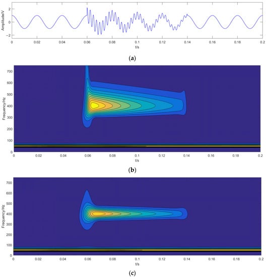
Figure 3.
Analysis results of transient oscillation. (a) The original signal of transient oscillation. (b) The analysis results of S-transform. (c) The analysis results of modified S-transform.
Figure 3a shows the original signal of transient oscillation. Figure 3b is the result of S-transform analysis. Figure 3c is the result of MST transform analysis. The results in Figure 3b,c are telling of the fact that the original signal is a superposition of sinusoidal and the modulated signal. The starting and ending time of oscillation signal disturbance (0.06 s and 0.14 s) can be more clearly seen from Figure 3b. Compared to the results shown in Figure 3b, the results using the MST method shown in Figure 3c present higher energy concentration in the entire TF maps, because of involvement of the energy concentration measure in the algorithm. Figure 3c indicates the starting time of oscillation signal disturbance is not clear enough, about 0.056 s, but the ending time is clear at 0.14 s. With continuous signal, the proposed algorithm does a very good job compared to the standard S-transform method. The comparisons confirm a better performance of the proposed method than standard S-transform.
4.3. Voltage Interruption
The voltage interruption signals can be given as: . In the time period of , the signal has voltage interruption. The analysis results of S-transform and modified S-transform are shown in Figure 4b,c, respectively.
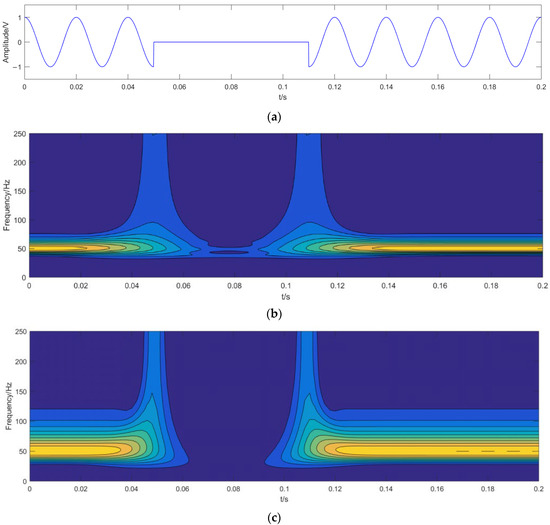
Figure 4.
Analysis results of voltage interruption. (a) The original signal of voltage interruption. (b) The analysis results of S-transform. (c) The analysis results of modified S-transform.
Figure 4a shows the original signal of voltage interruption in time domain. Figure 4b,c shows the analysis results of ST and MST in TF domain, respectively. The time sampling interval of the signal is 0.2 s. As is seen in Figure 4b, when the voltage is interrupted at 0.05 s, the frequency suddenly changes, and the amplitude decreases to the lowest at 0.06 s. However, due to the time resolution, the amplitude cannot decrease to 0. When the voltage recovers at 0.11 s, the frequency suddenly changes again, and the amplitude increases gradually. In Figure 4c, the frequency suddenly changes at the starting and ending time of voltage interruption (0.05 s and 0.11 s). At 0.06 s–0.10 s, the amplitude decreases to 0. The energy is more concentrated before the voltage interruption and after the voltage recovery. Comparison of the results shown in Figure 4b; the time resolution is improved and the frequency resolution is deteriorated in Figure 4c. The starting and ending time of voltage interruption (0.05 s and 0.11 s) can be clearly seen from Figure 4c. The proposed MST method presents higher energy concentrations in the TF map.
4.4. Voltage Sag and Voltage Swell with Harmonics
The voltage sag and voltage swell with harmonics signals can be given as: . The amplitude of increases by 0.6 in the time period of . The analysis results of S-transform and modified S-transform are shown in Figure 5b,c, respectively.
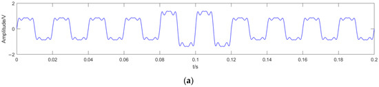
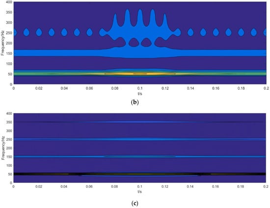
Figure 5.
Analysis results of voltage sag and voltage swell with harmonics. (a) The original signal of voltage sag and voltage swell with harmonics. (b) The analysis results of S-transform. (c) The analysis results of modified S-transform.
When the signal is different, its corresponding time-frequency resolution is different. Figure 5a is a multi-frequency signal source, which contains four frequency components of 50, 150, 250 and 350 Hz, respectively. The original signal of voltage sag and voltage swell with harmonics of is shown in Figure 5a. The time-frequency diagram of after ST and modified ST is shown in Figure 5b,c, respectively.
Figure 5a shows the original signal of voltage sag and voltage swell with harmonics. As a comparison, similar experiments were performed by S-transform method, and results are shown in Figure 5b. The results in Figure 5b,c are quite telling of the fact that the signal proposed algorithm does a very good job compared to the ST method. As shown in Figure 5b, the analysis results using ST method show the harmonic components of two frequencies, and they are 150 Hz and 250 Hz, respectively. The harmonic component of 350 Hz cannot be displayed. However, we can see that the amplitude of the signal increases obviously in the range of 0.07 s–0.13 s. Figure 5c shows the analysis results using the MST. A closer look at these results reveals that the frequency of harmonic components can be clearly seen from Figure 5c. The analysis results using MST method show the harmonic components of four frequencies, which are 50 Hz, 150 Hz, 250 Hz and 350 Hz, and the energy of signal component is relatively more concentrated. The amplitude of the signal increases from 0.055 s to 0.145 s, but the increase is not significant. The frequency resolution increases and the time resolution decreases by increasing the frequency. This means that the proposed MST method employs optimal windows in order to improve energy concentration while keeping the time and frequency resolution in an acceptable level. The comparisons confirm better energy concentration performance of the proposed method than ST. It can be seen that the MST method has high classification accuracy and high energy concentration.
5. Conclusions
To meet power quality requirements, it is necessary to classify and identify the power quality of the power grid connected with renewable energy generation. S-transform is an effective method to analyze power quality in time and frequency domains, and it is widely used to detect and classify various kinds of non-stationary power quality disturbances. However, the long taper and scaling criteria of the Gaussian window in SST will lead to poor time domain resolution at low frequency and poor frequency resolution at high frequency. To solve the effects, the optimal window function is proposed to locate the time frequency accurately in this paper. In this method, an improved window function for optimal energy concentration in time-frequency distribution is introduced. The method determines the parameters of the Gaussian window to improve the energy concentration in a time-frequency domain within a given time and frequency interval. On this basis, a window which can maximize the energy concentration in a finite time and frequency range is proposed. We demonstrate the performance of the proposed method and compare the results with those of SST. The comparisons better confirm performance of the proposed method compared to SST. Result shows that compared to SST with Gaussian window, ST based on the optimally concentrated window proposed in this paper has better energy concentration in time-frequency distribution.
Author Contributions
Conceptualization, K.L. and D.S.; methodology, D.S.; software, N.S. and D.S.; validation, K.L., N.S. and D.S.; formal analysis, D.S.; resources, K.L. and D.S.; data curation, D.S. and N.S.; writing-original draft preparation, D.S.; writing-review and editing, K.L. and D.S.; funding acquisition, K.L. All authors have read and agreed to the published version of the manuscript.
Funding
This research was funded by “Research on complex power quality disturbance identification and fault diagnosis based on deep learning”, grant number 52077089.
Institutional Review Board Statement
Not applicable.
Informed Consent Statement
Not applicable.
Data Availability Statement
The data presented in this study are available on request from the first author.
Conflicts of Interest
The authors declare no conflict of interest.
References
- Bullich-Massagué, E.; Ferrer-San-José, R.; Aragüés-Peñalba, M.; Serrano-Salamanca, L.; Pacheco-Navas, C.; Gomis-Bellmunt, O. Power plant control in large-scale photovoltaic plants: Design, implementation and validation in a 9.4 MW photovoltaic plant. IET Renew. Power Gener. 2016, 10, 50–62. [Google Scholar] [CrossRef] [Green Version]
- Muhammad, I.H.; Awang, J.; Makbul, A. Photovoltaic plant with reduced output current harmonics using generationside active power conditioner. IET Renew. Power Gener. 2014, 8, 817–826. [Google Scholar]
- Xie, N.; Luo, A.; Chen, Y.; Ma, F.; Xu, X.; Lu, Z.; Shuai, Z. Dynamic modeling and characteristic analysis on harmonics of photovoltaic power stations. Proc. CSEE 2013, 33, 10–17. [Google Scholar]
- Hu, H.; Shi, Q.; He, Z.; He, J.; Gao, S. Potential harmonic resonance impacts of PV inverter filters on distribution systems. IEEE Trans. Sustain. Energy 2015, 6, 151–161. [Google Scholar] [CrossRef]
- Xia, X.; Han, X. A novel active power filter for harmonic suppression and reactive power compensation. In Proceedings of the 2006 1ST IEEE Conference on Industrial Electronics and Applications, Singapore, 24–26 May 2006. [Google Scholar]
- Deokar, S.A.; Waghmare, L.M. Integrated DWT-FFT approach for detection and classification of power quality disturbances. Int. J. Electr. Power Energy Syst. 2014, 61, 594–605. [Google Scholar] [CrossRef]
- Jaramillo, S.H.; Heydt, G.T.; O’Neill-Carrillo, E. Power quality indices for aperiodic voltages and currents. IEEE Trans. Power Deliv. 2000, 15, 784–790. [Google Scholar] [CrossRef]
- Erişti, H.; Demir, Y. Automatic classification of power quality events and disturbances using wavelet transform and support vector machines. IET Gener. Transm. Distrib. 2012, 6, 968–976. [Google Scholar] [CrossRef]
- De Yong, D.; Magnago, F.; Magnago, F. An effective power quality classifier using wavelet transform and support vector machines. Expert Syst. Appl. 2015, 42, 6075–6081. [Google Scholar] [CrossRef]
- Afroni, M.J.; Sutanto, D.; Stirling, D. Analysis of nonstationary power-quality waveforms using iterative Hilbert Huang transform and SAX algorithm. IEEE Trans. Power Deliv. 2013, 28, 2134–2144. [Google Scholar] [CrossRef]
- Biswal, B.; Biswal, M.; Mishra, S.; Jalaja, R. Automatic classification of power quality events using balanced neural tree. IEEE Trans. Ind. Electron. 2014, 61, 521–530. [Google Scholar] [CrossRef]
- Griffin, D.; Lim, J. Signal estimation from modified short-time Fourier transform. IEEE Trans. Acoust. Speech Signal Process. 1984, 32, 236–243. [Google Scholar] [CrossRef]
- Stockwell, R.G.; Mansinha, L.; Lowe, R.P. Localization of the complex spectrum: The S-transform. IEEE Trans. Signal Process. 1996, 44, 998–1001. [Google Scholar] [CrossRef]
- Huang, N.; Xu, D.; Liu, X.; Lin, L. Power quality disturbances classification based on S-transform and probabilistic neural network. Neurocomputing 2012, 98, 12–23. [Google Scholar] [CrossRef]
- Jianmin, L.; Zhaosheng, T.; Qiu, T.; Junhao, S. Detection and classification of power quality disturbances using double resolution S-transform and DAG-SVMs. IEEE Trans. Instrum. Meas. 2016, 65, 2302–2312. [Google Scholar]
- Chakraborty, A.; Okaya, D. Frequency-time decomposition of seismic data using wavelet-based methods. Geophisics 1995, 60, 1906–1916. [Google Scholar] [CrossRef] [Green Version]
- Sahani, M.; Dash, P.K. Automatic Power Quality Events Recognition based on Hilbert Huang Transform and Extreme Learning Machine. IEEE Trans. Ind. Inform. 2018, 14, 3849–3858. [Google Scholar] [CrossRef]
- Boashash, B. Time frequency signal analysis: Past, present and future trends. Control Dyn. Syst. 1996, 78, 1–69. [Google Scholar]
- Cohen, L. Time frequency distribution-a review. Proc. IEEE 1989, 77, 941–981. [Google Scholar] [CrossRef] [Green Version]
- Orallo, C.M.; Carugati, I.; Maestri, S.; Donato, P. Harmonics measurement with a modulated sliding discrete Fourier transform algorithm. IEEE Trans. Instrum. Meas. 2014, 63, 781–793. [Google Scholar] [CrossRef]
- Kwok, H.K.; Jones, D.L. Improved instantaneous frequency estimation using an adaptive short-time Fourier transform. IEEE Trans. Signal Process. 2015, 48, 2964–2972. [Google Scholar] [CrossRef]
- Zhao, X.; Ye, B. Convolution wavelet packet transform and its applications to signal processing. Digit. Signal Process. N. Y. 2010, 20, 1352–1364. [Google Scholar] [CrossRef]
- Duan, Z.; Zhang, J.; Zhang, C.; Mosca, E. A simple design method of reduced-order filters and its applications to multirate filter bank design. Signal Process. 2006, 86, 1061–1075. [Google Scholar] [CrossRef]
- Ma, J.; Jiang, J. Analysis and design of modified window shapes for S-transform to improve time-frequency localization. Mech. Syst. Signal Process. 2015, 58, 271–284. [Google Scholar] [CrossRef]
- Li, J.; Yang, Y.; Lin, H.; Teng, Z.; Zhang, F.; Xu, Y. A voltage sag detection method based on modified S transform with digital prolate spheroidal window. IEEE Trans. Power Deliv. 2021, 36, 997–1006. [Google Scholar] [CrossRef]
- Mahela, O.P.; Shaik, A.G.; Khan, B.; Mahla, R.; Alhelou, H.H. Recognition of complex power quality disturbances using S-transform based ruled decision tree. IEEE Access 2020, 8, 173530–173547. [Google Scholar] [CrossRef]
- Djurovi, I.; Sejdi, E.; Jiang, J. Frequency-based window width optimization for S-transform. AEU-Int. J. Electron. Commun. 2008, 62, 245–250. [Google Scholar] [CrossRef]
- Zhang, S.; Li, P.; Zhang, L.; Li, H.; Jiang, W.; Hu, Y. Modified S transform and ELM algorithms and their applications in power quality analysis. Neurocomputing 2016, 185, 231–241. [Google Scholar] [CrossRef]
- Sejdi´c, E.; Djurovi´c, I.; Jiang, J. A window width optimized S transform. EURASIP J. Adv. Signal Process. 2008, 2008, 672941. [Google Scholar] [CrossRef] [Green Version]
- Yao, W.; Teng, Z.; Tang, Q.; Zuo, P. Adaptive Dolph-Chebyshev window-based S transform in time-frequency analysis. IET Signal Process 2014, 8, 927–937. [Google Scholar] [CrossRef]
- Pinnegar, C.R.; Mansinha, L. The bi-Gaussian S-transform. SIAM J. Sci. Comput. 2003, 24, 1678–1692. [Google Scholar]
- Simon, C.; Ventosa, S.; Schimmel, M.; Heldring, A.; Dañobeitia, J.J.; Gallart, J.; Manuel, A. The S-transform and its inverses: Side effects of discretizing and filtering. IEEE Trans. Signal Process 2007, 55, 49284937. [Google Scholar] [CrossRef] [Green Version]
- Qiu, W.; Tang, Q.; Liu, J.; Teng, Z.; Yao, W. Power Quality Disturbances Recognition Using Modified S Transform and Parallel Stack Sparse Auto-encoder. Electr. Power Syst. Res. 2019, 174, 105876. [Google Scholar] [CrossRef]
- Wang, Q.; Gao, J.; Liu, N.; Jiang, X. High-resolution seismic time-frequency analysis using the synchrosqueezing generalized S-Transform. IEEE Geosci. Remote Sens. Lett. 2018, 15, 374–378. [Google Scholar] [CrossRef]
- Brown, R.A.; Lauzon, M.L.; Frayne, R.F. A general description of linear time-frequency transforms and formulation of a fast, invertible transform that samples the continuous S-Transform spectrum nonredundantly. IEEE Trans. Signal Process. 2010, 58, 281–290. [Google Scholar] [CrossRef]
- Ali, M.; Zied, B.; Djaffar, O.A.; Alain, D. A new optimized Stockwell transform applied on synthetic and real non-stationary signals. Digit. Signal Process. 2015, 46, 226–238. [Google Scholar]
Publisher’s Note: MDPI stays neutral with regard to jurisdictional claims in published maps and institutional affiliations. |
© 2021 by the authors. Licensee MDPI, Basel, Switzerland. This article is an open access article distributed under the terms and conditions of the Creative Commons Attribution (CC BY) license (https://creativecommons.org/licenses/by/4.0/).