Abstract
Since the Industrial Revolution, human activities have led to the emission of a lot of greenhouse gases, such as carbon dioxide, sharply increasing the concentration of greenhouse gases in the atmosphere and resulting in serious global warming. With the rapid development of computer technology, the digital economy is gradually becoming the engine of economic growth. As a new economic mode, how the digital economy affects the environment is worth studying. In this paper, we introduced the digital economy into the Solow growth model as technological progress and conducted fixed-effects regressions based on the global panel data of 190 countries from 2005 to 2016. We found an inverted U-shaped, non-linear relationship between CO2 emissions and the digital economy, which supports the environmental Kuznets curve (EKC) hypothesis. We suggest that governments need to not only adopt hedging policies to reduce CO2 emissions caused by the digital economy in the early stage but also promote the development of the digital economy to achieve the goal of global collaborative environmental protection.
1. Introduction
The global environmental problems, such as the sharp reduction in forests, grassland degradation, desert expansion, frequent sandstorms, air pollution, species reduction, and the water crisis, are becoming increasingly serious. These problems affect all aspects of human life. Since the Industrial Revolution, human activities have led to the emission of a lot of greenhouse gases, such as carbon dioxide, sharply increasing the concentration of greenhouse gases in the atmosphere and resulting in serious global warming. The Global Warming of 1.5 °C report released by the Intergovernmental Panel on Climate Change warns that the global mean surface temperature would increase between 3 and 4 °C (5.4 and 7.2 °F) by 2100 if carbon emissions continue at their current rate, leading to increasing extinction of plant and animal species, a shift in the patterns of agriculture, and a rise in sea levels.
Figure 1 shows the data of carbon dioxide emissions (metric tons per capita) collected from the World Bank. We can see that the global CO2 emissions are on the rise as a whole. In 1961, the global CO2 emissions were 2.99 metric tons per capita, and in 2012, they increased to 4.75 metric tons per capita.
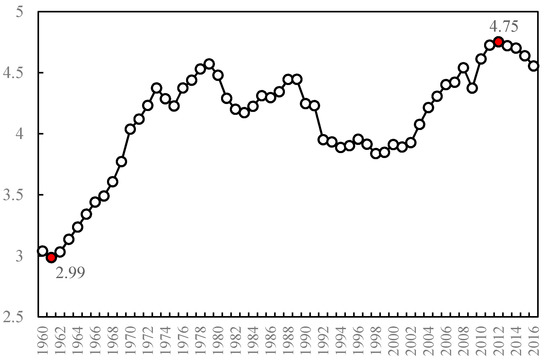
Figure 1.
Global CO2 emissions, 1960–2016.
Although natural factors, such as topography and climate, affect air quality, there is no doubt that the explosive economic activities and population growth since the Industrial Revolution are the main sources of air pollution and global warming. The living pollution caused by the increase in population, the industrial pollution caused by the increase in factories, and the traffic pollution caused by the rapid development of transportation have produced a lot of air pollution [1], making the environment unsustainable.
Since the 1990s, computer technology has been maturing. Artificial intelligence, blockchain technology, and 5G technology have led to many new economic modes, such as the digital economy. The digital economy is an economic form that guides and realizes the rapid optimal allocation and regeneration of resources and achieves high-quality economic development through the identification, selection, filtering, storage, and use of big data. The US Department of Commerce published the first research report about the digital economy on 15 April 1998, which focused on the decisive role of information as a core resource in the macro- and the micro-economy. Since then, the digital economy has rapidly become the engine of economic growth in the new millennium [2]. Figure 2 shows the international trade trend in digitally delivered services (US dollars at current prices in billions) collected by the United Nations Conference on Trade and Development (UNCTAD). Global international trade in digitally delivered services has been rising steadily since 2005. The export of digitally delivery services increased from USD 918 billion in 2005 to USD 3150 billion dolars in 2019, while their import increased from USD 792 billion in 2005 to USD 2774 billion in 2019.
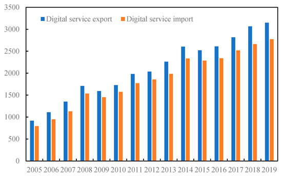
Figure 2.
International trade in digitally deliverable services, 2005–2019.
Information and communication technologies (ICT) are becoming increasingly important for businesses, consumers, and governments in all sectors of the economy around the world. After reading the COVID-19 economic stimulus plans, almost all the world’s major economies have listed “green” and “digital” as the two keywords of major policy directions. The digital economy, especially ICT, as an example technological progress, has created opportunities for sustainable development and economic recovery in recent crises [3].
Therefore, this paper studied the impact of the digital economy on CO2 emissions. We introduced the digital economy into the Solow growth model as a kind of technological progress and built a dynamic equilibrium model between CO2 emissions and the digital economy. Due to the technological progress brought by the digital economy, enterprises reset production equipment and increase output in the early stage of economic development, thus increasing CO2 emissions. When the economy develops to a higher level, the output of enterprises is stable, and the cost of pollution treatment reduces due to digitalization, thus reducing CO2 emissions. Based on the fixed-effects model of the global panel data of 190 countries from 2005 to 2016, the empirical results show that there is an inverted U-shaped relationship between CO2 emissions and the digital economy, which is consistent with the EKC hypothesis.
This paper enriches the theoretical and empirical studies on the impact of the digital economy on CO2 emissions and draws a general and universal conclusion to support the EKC hypothesis. The rest of the paper is divided into the following sections: Section 2 describes the literature review and highlights the originality of this paper by comparing it with other studies. Section 3 explains the Solow growth model. Section 4 describes the development of an empirical model and data selection. Section 5 discusses empirical results. Section 6 compares this study with other related studies, discusses the limitations of our method and the methodology adopted, concludes the paper, and specifies proper policy implications.
2. Literature Review
There are many studies on the impact of economic activities on the environment. Kuznets [4] first found an inverted U-shaped relationship between environmental pollution and economic growth, that is, environmental pollution increases with the increase in income and decreases after reaching the peak or threshold point [5,6,7]. However, there are certain conditions for the EKC hypothesis. Dinda [8] says that only the relationship between the air quality index and economic growth shows the EKC phenomenon.
In addition to the impact of the overall economic growth on the environment, different forms of economic activities also have an impact on CO2 emissions. However, this impact is controversial. First, some researchers believe that urbanization accelerates carbon emissions [9]. The aim of low-carbon urbanization is to stabilize the speed of urbanization [10]. Other studies suggest that urbanization can effectively curb carbon emissions [11,12,13]. There is a non-linear relationship between urbanization and carbon emissions [14,15]. Second, the impact of the Foreign Direct Investment (FDI) on carbon dioxide emissions is different in different regions [16]. The FDI in some countries increases CO2 emissions [17,18], while the FDI in other countries inhibits CO2 emissions [19,20]. Different types of FDI have different effects on CO2 emissions. The labor-based FDI has a significant negative spillover effect, while the capital-based FDI has a significant positive spillover effect [21,22]. Third, some studies suggest that industrial agglomeration has expanded the production scale of factories, thus increasing pollution [23,24,25], while other studies suggest that industrial agglomeration can accelerate environmental innovation and improve energy use efficiency, thus reducing pollution [26,27]. Still others believe that the relationship between industrial agglomeration and air pollution is uncertain: the relationship between industrial agglomeration and sulfur dioxide emissions has an inverted U shape [28], and the relationship between industrial agglomeration and industrial wastewater and dust has an S shape [29].
With the development of computer technology, studies on the impact of digital economy on the environment and sustainable development are increasing.
First, the use of digitalization can promote sustainable economic development. Sudoh [30] says that with the threat of global environmental degradation becoming increasingly serious, global digital networks, which can link regions around the world and foster new social norms to overcome nationalist interests, may play an important role in the long term. Martynenko [31] believes that digitalization brings about ecological modernization of production, which can ensure not only the saving of various resources but also the sustainable development of territories, countries, and the global society. Qian et al. [32] believe that the green economy and the digital economy can promote each other. On the one hand, the digital economy can effectively promote green transformation of the global economy. On the other hand, the green economy can also help the digital economy realize green, low-carbon, and sustainable development.
Second, although the Internet has great potential to improve the environment, the digital economy also has negative impacts on the environment [33]. Shvakov and Petrova [34] studied the data of the top 10 countries in the world in 2019 and found that digitization does not contribute to the development of a green or an energy-saving economy but hinders their development. In addition, the implementation of global sustainable development goals requires limiting the growth rate of the digital economy.
Finally, there is a non-linear relationship between the digital economy and air pollution. Wu et al. [35] reported an inverted U-shaped relationship between the digital economy and SO2 emissions by testing the provincial panel data of China from 2011 to 2017. The digital economy has a positive effect on the environment in China’s developed regions and a negative effect in less developed regions.
By analyzing the studies on the impact of the digital economy on the environment, we find that most of the studies at this stage are qualitative in nature. They investigate the impact of the digital economy on the environment mainly using descriptive analysis, which lacks theoretical and mathematical models. In addition, quantitative studies and empirical tests are only conducted on specific countries, lacking universality and generality. There is also no consensus on whether the digital economy is conducive to sustainable development.
In this paper, we establish a new partial equilibrium growth model of CO2 emissions and the digital economy by introducing the digital economy as technological progress based on Taylor [36] and Bai and Chen [37] and draw out an EKC curve of CO2 emissions and the digital economy. We also use country panel data to examine the U-shaped curve between CO2 emissions and the digital economy and determine whether the impact of the digital economy on CO2 emissions is heterogeneous among countries.
3. Theoretical Model
3.1. Hypothesis of Production Function
Assume that the production function of a firm is a Harold’s neutral technological progress function [38] written as Equation (1):
where Y is the total output, K is the total amount of capital, L is the total amount of labor, and D is the firm’s digitalization level (i.e., technological progress) followed by Bai and Chen [37]. Digitalization can optimize the allocation of production factors and improve labor productivity. Assume that the production function is constant returns to scale and diminishing marginal productivity. Every factor of production is essential, and it is a second-order neoclassical production function, which is continuously differentiable and satisfies the conditions [39] written as the following Equation (2) to Equation (4).
According to the assumption of constant returns to scale, the production function can be rewritten in intensive form as Equation (5):
where is the capital stock of the effective labor per capita and is expressed as the output of the effective labor per capita. Equation (5) shows the functional relationship between the effective capital per capita and the effective output per capita.
Assume that the labor population grows at the rate of n as Equation (6) and the digitalization degree (labor productivity) increases at the speed of gD as Equation (7):
3.2. Dynamic Behavior and Equilibrium State of the Economy
When the commodity market is in equilibrium, investment equals saving. According to Taylor [39], we set the capital accumulation equation of the whole economy as Equation (8):
where s is a fixed savings rate and capital accumulates via savings and precedes at rate δ. E is the cost of CO2 treatment formulated as Equation (9), where Z is the CO2 emissions of the firm, which is related to the output level, and θ is the treatment cost of CO2 emissions per unit. Similarly, an intensive form of the CO2 treatment cost equation can be obtained as Equation (10):
Substituting Equations (9) and (10) into Equation (8) and dividing both sides of Equation (8) by K, we get Equation (11):
Therefore, the dynamic equation of the effective capital per capita is written as Equation (12). Equation (13) is obtained by sorting out Equation (12):
When the economy is in equilibrium, the growth rate of the effective capital per capita is 0, which means . Therefore, the relationship between the effective CO2 emissions per capita and capital per capita and digitalization per capita is determined by Equation (14). In addition, the growth rate of digitalization, gD, and the population growth rate n remain unchanged in the steady state, which means both grow at a stable rate.
In Equation (14), the effective CO2 emissions per capita are on the left side. On the right side, the first item implies that the output increases due to continuous capital accumulation, thus increasing CO2 emissions. The second item on the right side implies that the CO2 emissions in the production process are decreasing with the continuous improvement of digitalization.
The implication of Equation (14) was better understood by drawing Figure 3. In Figure 3a, the initial effective capital per capita is 0, which means the firm does not produce and CO2 emissions are zero. In the early stage of economic development (or in the early stage of digitization), the amount of CO2 emissions caused by the firm’s large-scale production is larger than that reduced by digitalization and the speed of CO2 emitting is faster than that of CO2 processing (curve OA). When the economy continues to develop, the digitalization level improves. The amount of CO2 emissions is still greater than that reduced by digital technology progress, but the speed of CO2 emissions is slower than that of CO2 treatment (curve AB). When the economy further develops, the digitalization level further improves. The amount of CO2 emitted by the firm is less than that reduced by digitalization, which means digitalization can not only reduce air pollution emissions but also improve the surrounding environment through technology spillover and other effects. Figure 3b is an inverted U-shaped relationship between CO2 emissions and digitalization drawn from Figure 3a and implies that, with the development of digitalization, CO2 emissions first rise and then fall, which is consistent with the EKC hypothesis.
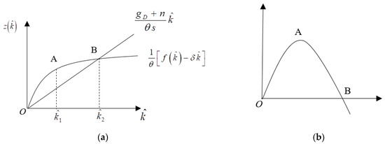
Figure 3.
Relationship between CO2 emissions and digitalization. (a) Relationship between CO2 emissions and effective capital per capita. (b) EKC curve of CO2 emissions and digitalization.
4. Empirical Model, Variable Description, and Data
According to the theoretical model, we put forward the following hypothesis. In this section, we tested this hypothesis empirically.
Hypothesis:
There is an inverted U-shaped relationship between CO2 emissions and the digital economy. In the early stage of digital economy development, CO2 emissions increase to the peak. With further development of the digital economy, CO2 emissions decrease.
4.1. Variable Description and Data
We collected the data of CO2 emissions per capital from 1960 to 2016 given by the World Bank and obtained the smoothing variable lnCO2 as the dependent variable after taking the natural logarithm. We also collected the export and import data of digitally delivered services from 2005 to 2019 given by UNCTAD, added the data, and divided them by the total annual population of the corresponding country to obtain a measure of the international trade of digitally deliverable services per capita. The data of the total population was collected from the World Bank. The smoothing variable lndigital was obtained after taking the natural logarithm. We squared lndigital to obtain the core independent variable (lndigital)2.
As the global data of CO2 emissions lasted from 1960 to 2016, and that of the international trade of digitally delivered services from 2005 to 2019, we obtained the unbalanced panel data of 190 countries from 2005 to 2016 due to data availability. Chow and Li [40] used the data of 132 countries from 1992 to 2004 to perform empirical tests and support the EKC hypothesis conclusively, so we used global data from 2005 to 2016 in this study. In addition, similar to Adekunle [41] and Quayes [42], who successfully used unbalanced panel data to conduct sustainability research, we did, too.
The following five variables were selected as control variables: the natural logarithm of the GDP per capita (lngdpp), the natural logarithm of the foreign direct investment per capita (lnIO), the industrialization level (Industry), the urbanization level (Urban), and the power supply level (Electricity). We added the outflows and inflows of the foreign direct investment and then divided it by the total population and took the natural logarithm to obtain the variable lnIO. The industrialization level (Industry) was characterized by the proportion of industrial value in the GDP, the urbanization level (Urban) by the proportion of urban population in the total population, and the power supply level (Electricity) by population access to electricity in the total population. All the control variables were collected from the World Bank. The descriptive statistics of the variables are shown in Table 1.

Table 1.
Descriptive statistics of core variables.
4.2. Empirical Model Selection
The impact of the digital economy on air pollution was studied by choosing CO2 emissions per capita as the dependent variable and the square of the digitally deliverable service trade per capita as the independent variable to measure the development level of the digital economy. We focused on the coefficient ꞵ2 of the core independent variable (lndigital)2 to determine whether it is significantly negative to test the inversed U-shaped relationship between CO2 emissions and the digital economy. The model was constructed as the following Equation (15), according to Neagu [43], which is consistent with the theoretical model:
where i represents the i-th country, t represents the t-th year, lnCO2 is the dependent variable, (lndigital)2 is the core explanatory variable, and X represents the control variables lngdpp, lnIO, Industry, Urban, and Electricity.
In the light of the differences among different countries, we first constructed a panel variable coefficient model and selected the optimal model based on model estimation results. In addition, individual fixed effects or individual random effects were chosen when constructing the model. The fixed-effects model is written as Equation (16), according to Zhang et al. [44], where Countryi captures the country fixed effect and yeart the year fixed effect as follows:
The random-effects model is written as Equations (17) and (18) as follows:
To decide which model is much more appropriate, we performed the Hausman test. The null hypothesis was that there is no significant difference in the estimators between the fixed-effects and the random-effects model. If the null hypothesis is rejected, the conclusion is that the random-effects model is not appropriate, because the random effects may be related to one or more regressors. In this case, the fixed-effects model was better than the random-effects model. The result of the Hausman test is shown in Table 2. According to the Hausman test (probability < 0.10), we built a fixed-effects model.
Table 2.
Results of the Hausman test.
Regarding the country panel data, there may be cross-section dependence and slope heterogeneity in the sample. It is better to test cross-section dependence and slope heterogeneity before choosing the final regression model. If the panel data have the property of cross-section dependence and slope heterogeneity, common correlated effects mean group (CCEMG) and augmented mean group (AMG) estimators need to be applied. However, the sample data in this study were too unbalanced to perform the two tests mentioned above and the square terms in the model were not well applied to the tests. Therefore, we chose the fixed-effects model to meet the need of short unbalanced data and square terms. In addition, to solve the problem of heteroscedasticity and sequence autocorrelation in panel data, the fixed-effects regression was clustered to country and year levels according to Azzimonti [45].
5. Estimated Results and Discussion
5.1. Basic Regression Results
The basic fixed-effects regression results of Equation (16) are shown in Table 3. There are no control variables in column 1 of Table 3. As shown in column 1, (lndigital)2 was −0.013, and it was significant at the 1% level, indicating an inverted U-shaped relationship between CO2 emissions and the digital economy. CO2 emissions will first rise and then decrease with the development of the digital economy, which is consistent with the conclusion of the theoretical model and supports the EKC hypothesis. After adding control variables one by one from columns 2 to 6, the number of regression countries dropped from 190 to 178 because some control variables of countries were missing available data (the same data availability problem exists in Table 4). As shown in columns 2 to 6, (lndigital)2 remained negative, the coefficient value was relatively stable, and was significant at the 1% level, which means that the inverted U-shaped relationship between CO2 emissions and digital economy will not change with an increase in control variables.
Table 3.
Basic results of CO2 emissions and the digital economy.
Table 4.
Robustness tests of CO2 emissions and the digital economy.
We can find the turning point by taking the derivative with respect to lndigital of all the estimated equations and equating it to zero. For the coefficients estimated in column 1 of Table 3, the turning point of lndigital was 4.58, which means that when the trade of digitally delivered services per capita rises to 97.51 dollars per capita, CO2 emissions will start decreasing from that point with continuous improvement of digitalization. After considering other control variables, the turning point of lndigital in column 6 was 2.92, lower than that in column 1. This is consistent with the economic institution because some of the CO2 emissions are absorbed by control variables. The turning point calculated in column 6 implies that CO2 emissions will start decreasing from the point that the trade of digitally delivered services per capita rises to 18.54 dollars per capita.
The actual average of digitally delivered services per capita was USD 190.76 per capita according to Table 1 (5.251). Comparing the turning point calculated above with the actual number in Table 1 showed that the sample countries are in the decreasing phase of the curve, which means digitalization can not only reduce air pollution emissions but also improve the surrounding environment through technology spillover effects in the sample countries.
5.2. Robustness Test and Group Test
To ensure the reliability of basic regression results, we carried out the robustness test shown in Table 4. In columns 1 and 2 of Table 4, we added the export and import of ICT services given by UNCTAD and divided it by the total population to obtain the trade of ICT per capita. We replaced (lndigital)2 and lndigital by (lnICT)2 and lnICT, respectively, and used (lnICT)2 as the core independent variable to perform the first robustness check. Column 1 does not include control variables, while column 2 includes all control variables. The (lnICT)2 value was negative, indicating an inverted U-shaped relationship between CO2 emissions and ICT, which is consistent with the basic regression results.
We used Fine Particulate Matter (PM2.5) data given by the World Bank to replace CO2 emissions for the second robustness test in columns 3 and 4. The results showed an inverted U-shaped relationship between PM2.5 and the digital economy. Moreover, the regression coefficients of (lndigital)2 in columns 3 and 4 of Table 4 were −0.375 and −0.354, respectively, whose absolute values are larger than those in columns 1 and 6 of Table 3. This implies that PM2.5 increases faster than CO2 emissions with the development of the digital economy before the turning point and that it also decreases faster than CO2 emissions in the decline stage.
In columns 5 and 6, we used PM2.5 as the explained variable and ICT as the explanatory variable for the third robustness test. The square terms remained negative and were significant at the 5% level. The regression coefficients of the square terms in columns 5 and 6 of Table 4 were also absolutely larger than those in columns 1 and 2. Table 4 proves that there is an inverted U-shaped relationship between CO2 emissions and the digital economy, and the regression results are robust.
For further analysis, we conducted group regression by dividing the countries into different income groups according to the World Bank classification. The World Bank divides countries into four groups by income: high income, upper middle income, lower middle income, and low income. As the development of the digital economy in high-income and upper-middle-income groups is faster than that in lower-middle-income and low-income groups, we divided the existing data into the following two groups: (i) high-income and upper-middle-income and (ii) low-income and lower-middle-income. The group regression results are shown in Table 5. The coefficient of the core explanatory variable (lndigital)2 in the high-income and upper-middle-income group was -0.010, which was significant at the 5% level and nearly the same as the world level in column 6 of Table 3. The coefficient of the core explanatory variable (lndigital)2 in the low-income and lower-middle-income group was negative but not significant. This is because the development of the digital economy in low-income and lower-middle-income countries is low, so the non-linear relationship between CO2 emissions and the digital economy is not significant.
Table 5.
Group test of CO2 emissions and the digital economy.
The coefficients of the control variable lngdpp in both groups were significant at the 1% level, which means that the development of the GDP will increase CO2 emissions. The impact of the per capita GDP on CO2 emissions is smaller in the high-income and upper-middle-income group than that in column 6 of Table 3, while the impact of the per capita GDP on CO2 emissions is larger in the low-income and lower-middle-income group than that in column 6 of Table 3. For the high-income and upper-middle-income countries, access to electricity increases CO2 emissions, whose coefficient was larger than that in column 6 of Table 3. For low-income and lower-middle-income countries, FDI development also increases CO2 emissions, whose coefficient was larger than that in column 6 of Table 3.
5.3. Endogeneity Test
To avoid the endogeneity caused by reciprocal causation between CO2 emissions and the digital economy, we applied the instrumental variables (IV)-two-stage least-squares (2SLS) method. Following Song et al. [46], we used the first-order lag term of (lndigital)2 as an instrumental variable to check the reliability of the basic results.
Table 6 shows the regression results by using the instrumental variable. We used the Durbin–Wu–Hausman test (DWH test) to check whether the independent variable (lndigital)2 is endogenous. If the p-value of the DWH test is <0.05 or 5%, then the variable is endogenous. Table 6 shows that the endogeneity of (lndigital)2 exists in columns 2 and 3. Although the result of the endogenous test was uncertain from the statistical aspect, reciprocal causation between CO2 emissions and the digital economy has economic implications. Therefore, we still used the instrumental variables (IV)-two-stage least-squares (2SLS) method to solve the endogeneity problem.
Table 6.
Endogeneity test of CO2 emissions and the digital economy.
Table 6 shows a stable, inverted U-shaped relationship between CO2 emissions and the digital economy, and it was significant at the 1% level. The regression coefficient from columns 1 to 6 was consistent with the basic regression results. The turning points of lndigital in columns 1 and 6 of Table 6 were 4.25 and 3, respectively, which is similar to the values in Table 3 (4.58 and 2.52, respectively). When the trade of digitally delivered services per capita rises to 70.11 dollars per capita (column 1), CO2 emissions will start decreasing from that point with continuous improvement of digitalization. When the trade of digitally delivered services per capita rises to USD 20.29 per capita (column 6), CO2 emissions will start decreasing from that point. Therefore, the finding of an inverted U-shaped relationship between CO2 emissions and the digital economy is reliable and credible after controlling for endogeneity in the model.
6. Discussion and Conclusions
6.1. Discussion
By establishing a mathematical model and conducting empirical tests, we found that there is an inverted U-shaped relationship between CO2 emissions and the digital economy. In the early stage of digitalization, CO2 emissions continue to increase. When the digitalization increases to a higher level, CO2 emissions begin to decrease after reaching a peak. Wu et al. [35] and Bai and Chen [37] used the square term of the digital economy index in the empirical model to test the EKC hypothesis of the digital economy and SO2 emissions, and their results were similar to ours.
However, there are some differences. First, Bai and Chen [37] used China’s provincial panel data from 2012 to 2018, and Wu et al. [35] used China’s provincial panel data from 2011 to 2017. Their samples were small and limited to one country. Our study extended the sample into all the countries available. Second, Bai and Chen [37] established a production decision model to describe the pollution emission behavior of enterprises under digitalization, so there was no equilibrium, and the market did not clear, while we established a partial equilibrium growth model of CO2 emissions and the digital economy.
This study had some limitations. First, we considered digitalization as the only technological progress in our theoretical analysis to simplify the model. Some other technologies may exist in practice, which might reduce CO2 emissions. In a future study, the interaction impact of different technologies on CO2 emissions needs to be incorporated into the theoretical model. Second, limited by the availability of data, we used the panel data from 2005 to 2016 for empirical tests, which is not sufficient. If there are more available data or longer data at the global level, the conclusion of this study needs to be empirically tested again in the future to check the robustness. Finally, we failed to perform the cross-section dependence test proposed by Pesaran [47] and the slope heterogeneity test proposed by Pesaran and Yamagata [48] due to unbalanced data and the square term in the regression model. The common correlated effects mean group (CCEMG) estimator proposed by Pesaran [49] and the augmented mean group (AMG) estimator developed by Eberhardt and Teal [50] need to be used to conduct empirical tests in the future when the global data of the digital economy become much more complete.
6.2. Conclusions
Global warming is becoming increasingly serious, which is closely related to human economic activities. Since the 1990s, computer technology has developed rapidly, forming a new economic operation mode, such as the digital economy. What is the impact of the digital economy on global warming? Does it also satisfy the environmental Kuznets curve? This paper studied the impact of the digital economy on CO2 emissions.
In the theoretical model, digitization was introduced into the Solow growth model as a kind of technological progress. By establishing a dynamic equation of capital accumulation, the relationship between CO2 emissions and digitization degree was solved. The model showed an inverted U-shaped relationship between CO2 emissions and the digitalization, which is consistent with the EKC hypothesis. At the beginning of digitalization, firms produce more goods because of technological progress, thus releasing more CO2 emissions, which are greater than the reduction of CO2 due to digitalization. When the digitalization level is high, the treatment amount of CO2 is greater than CO2 emissions, as firms produce goods at a stable level and technological progress leads to green economy.
This paper used global panel data of 190 countries from 2005 to 2016 to perform fixed-effects regression. The results of basic regression showed that the square term of the digital economy is negative and significant at the 1% level, which indicates an inverted U-shaped relationship between CO2 emissions and the digital economy. The robustness and endogeneity tests also supported the conclusion, which is consistent with the theoretical model. By dividing countries into two groups according to the World Bank classification, we found that the inverted U-shaped relationship between CO2 emissions and the digital economy in the high-income and upper-middle-income group is significant, while that in the low-income and lower-middle-income group is not significant.
According to the results of this study, we propose a few relevant policy implications. First, at the beginning of digitalization, the development of the digital economy will increase CO2 emissions. Therefore, governments need to adopt hedging policies to mitigate the adverse effects of the digital economy in order to prevent industrial CO2 emissions. Second, when the development of the digital economy reaches a certain level, CO2 emissions can be effectively alleviated. Therefore, all countries should adhere to the development of the digital economy to shorten the pollution time caused by it in the early stage and make better use of it to achieve the goal of global collaborative environmental protection. Third, high-income and upper-middle-incomes countries should take full use of the digital economy to reduce CO2 emissions, while low-income and lower-middle-income countries should be alert to CO2 emissions in the development of the digital economy and adopt suitable policies to mitigate adverse effects.
Author Contributions
Conceptualization, X.L., J.L., and P.N.; methodology, X.L., J.L., and P.N.; formal analysis, X.L., J.L., and P.N.; data curation, X.L., J.L., and P.N.; writing—original draft preparation, X.L., J.L., and P.N.; writing—review and editing, X.L., J.L., and P.N. This study is the result of teamwork. All authors equally contributed to designing the study, analyzing the data, writing the draft, and revising the study. Authors are ranked alphabetically by their last names. All authors have read and agreed to the published version of the manuscript.
Funding
This research received no external funding.
Institutional Review Board Statement
Not applicable.
Informed Consent Statement
Not applicable.
Data Availability Statement
The study did not report any additional data.
Conflicts of Interest
The authors declare no conflict of interest.
References
- Ang, J.B. CO2 Emissions, Energy Consumption, and Output in France. Energy Policy 2007, 35, 4772–4778. [Google Scholar] [CrossRef]
- Tapscott, D.; Lowy, A.; Ticoll, D. Blueprint to the Digital Economy: Wealth Creation in the Era of e-Business, 1st ed.; McGraw-Hill: New York, NY, USA, 1998; p. 384. [Google Scholar]
- Ciocoiu, C.N. Integrating digital economy and green economy: Opportunities for sustainable development. Theor. Empirica. 2011, 6, 33–43. [Google Scholar]
- Kuznets, S. Economic Growth and Income Inequality. Am. Econ. Rev. 1955, 45, 1–28. [Google Scholar]
- Grossman, G.; Krueger, A. Economic environment and the economic growth. Q. J. Econ. 1995, 110, 353–377. [Google Scholar] [CrossRef] [Green Version]
- Friedl, B.; Getzner, M. Determinants of CO2 emissions in a small open economy. Ecol. Econ. 2003, 45, 133–148. [Google Scholar] [CrossRef]
- Managi, S.; Jena, P.R. Environmental productivity and Kuznets curve in India. Ecol. Econ. 2008, 65, 432–440. [Google Scholar] [CrossRef]
- Dinda, S. Environmental Kuznets curve hypothesis: A survey. Ecol. Econ. 2004, 49, 431–455. [Google Scholar] [CrossRef] [Green Version]
- Madlener, R.; Sunak, Y. Impacts of urbanization on urban structures and energy demand: What can we learn for urban energy planning and urbanization management? Sustain. Cities Soc. 2011, 1, 45–53. [Google Scholar] [CrossRef]
- Wang, Y.; Li, L.; Kubota, J.; Han, R.; Zhu, X.; Lu, G. Does urbanization lead to more carbon emission? Evidence from a panel of BRICS countries. Appl. Energy 2016, 168, 375–380. [Google Scholar] [CrossRef]
- Liddle, B. Demographic dynamics and per capita environmental impact: Using panel regressions and household decomposi-tions to examine population and transport. Popul. Environ. 2004, 26, 23–39. [Google Scholar] [CrossRef]
- Chen, H.; Jia, B.; Lau, S.S.Y. Sustainable urban form for Chinese compact cities: Challenges of a rapid urbanized economy. Habitat. Int. 2008, 32, 28–40. [Google Scholar] [CrossRef]
- Ewing, R.; Rong, F. The impact of urban form on US residential energy use. Hous. Policy Debate 2008, 19, 1–30. [Google Scholar] [CrossRef]
- Liu, Y.; Yan, B.; Zhou, Y. Urbanization, economic growth, and carbon dioxide emissions in China: A panel cointegration and causality analysis. J. Geogr. Sci. 2016, 26, 131–152. [Google Scholar] [CrossRef] [Green Version]
- Ji, X.; Chen, B. Assessing the energy-saving effect of urbanization in China based on stochastic impacts by regression on pop-ulation, affluence and technology (STIRPAT) model. J. Clean. Prod. 2017, 163, S306–S314. [Google Scholar] [CrossRef]
- Peng, H.; Tan, X.; Li, Y.; Hu, L. Economic growth, foreign direct investment and CO2 emissions in China: A panel granger causality analysis. Sustainability 2016, 8, 233. [Google Scholar] [CrossRef] [Green Version]
- Pao, H.; Tsai, C. Multivariate Granger causality between CO2 emissions, energy consumption, FDI (foreign direct investment) and GDP (gross domestic product): Evidence from a panel of BRIC (Brazil, Russian Federation, India, and China) countries. Energy 2011, 36, 685–693. [Google Scholar] [CrossRef]
- Behera, S.R.; Dash, D.P. The effect of urbanization, energy consumption, and foreign direct investment on the carbon dioxide emission in the SSEA (South and Southeast Asian) region. Renew. Sust. Energ. Rev. 2017, 70, 96–106. [Google Scholar] [CrossRef]
- Shaari, M.S.; Hussain, N.E.; Abdullah, H.; Kamil, S. Relationship among foreign direct investment, economic growth and CO2 emission: A panel data analysis. Int. J. Energy Econ. Policy 2014, 4, 706–715. [Google Scholar]
- Keho, Y. Is foreign direct investment good or bad for the environment? Times series evidence from ECOWAS countries. Econ. Bull. 2015, 35, 1916–1927. [Google Scholar]
- Tang, C.F.; Tan, B.W. The impact of energy consumption, income and foreign direct investment on carbon dioxide emissions in Vietnam. Energy 2015, 79, 447–454. [Google Scholar] [CrossRef]
- Hu, J.; Wang, Z.; Lian, Y.; Huang, Q. Environmental regulation, foreign direct investment and green technological progress-Evidence from Chinese manufacturing industries. Int. J. Environ. Res. Public Health 2018, 15, 221. [Google Scholar]
- Virkanen, J. Effect of urbanization on metal deposition in the bay of Töölönlahti, Southern Finland. Mar. Pollut. Bull. 1998, 36, 729–738. [Google Scholar] [CrossRef]
- Duc, T.; Vachaud, G.; Bonnet, M.P.; Prieur, N.; Loi, V.D.; Anh, L.L. Experimental investigation and modelling approach of the impact of urban wastewater on a tropical river; a case study of the Nhue River, Hanoi, Viet Nam. J. Hydrol. 2007, 334, 347–358. [Google Scholar] [CrossRef]
- Cheng, Z. The spatial correlation and interaction between manufacturing agglomeration and environmental pollution. Ecol. Indic. 2016, 61, 1024–1032. [Google Scholar] [CrossRef]
- Zeng, D.; Zhao, L. Pollution havens and industrial agglomeration. J. Environ. Econ. Manag. 2009, 58, 141–153. [Google Scholar] [CrossRef] [Green Version]
- Effiong, E.L. On the urbanization-pollution nexus in Africa: A semiparametric analysis. Qual. Quant. 2018, 52, 445–456. [Google Scholar] [CrossRef]
- He, C.; Huang, Z.; Ye, X. Spatial heterogeneity of economic development and industrial pollution in urban China. Stoch. Environ. Res. Risk Assess. 2014, 28, 767–781. [Google Scholar] [CrossRef]
- Zhang, K.; Dou, J. Agglomeration and pollution: Empirical analysis based on the 287 cities of China. J. Financ. Res. 2015, 12, 32–45. [Google Scholar]
- Sudoh, O. The Knowledge Network in the Digital Economy and Sustainable Development. In Digital Economy and Social De-sign, 1st ed.; Springer: Tokyo, Japan, 2005; pp. 3–38. [Google Scholar]
- Martynenko, T.S.; Vershinina, I.A. Digital economy: The possibility of sustainable development and overcoming social and environmental inequality in Russia. Revista Espacios 2018, 39, 12. [Google Scholar]
- Qian, L.; Fang, Q.; Lu, Z. Research on the Synergy of Green Economy and Digital Economy in Stimulus Policies. Southwest Financ. 2020, 473, 3–13. [Google Scholar]
- Sui, D.Z.; Rejeski, D.W. Environmental impacts of the emerging digital economy: The E-for-environment E-commerce? Environ. Manag. 2002, 29, 155–163. [Google Scholar] [CrossRef]
- Shvakov, E.E.; Petrova, E.A. Newest Trends and Future Scenarios for a Sustainable Digital Economy Development. In Scientific and Technical Revolution: Yesterday, Today and Tomorrow, 1st ed.; Popkova, E., Sergi, B., Eds.; Springer: Cham, Switzerland, 2009; pp. 1378–1385. [Google Scholar]
- Wu, Y.; Luo, C.; Luo, L. The impact of the development of the digital economy on Sulfur Dioxide emissions: Empirical evidence based on provincial panel data. J. Wuhan Polytech. 2021, 20, 82–88. [Google Scholar]
- Taylor, W. The Green Solow Model. J. Econ. Growth 2010, 15, 127–153. [Google Scholar]
- Bai, L.; Chen, X. Research on the synergy of green economy and digital economy in stimulus policies. J. Dongbei Univ. Financ. Econ. 2020, 131, 73–81. [Google Scholar]
- Harrod, R.F. Toward a Dynamic Economics: Some Recent Developments of Economics Theory and Their Applications to Policy, 1st ed.; Macmillan: London, UK, 1942. [Google Scholar]
- Inada, K. Some structure characteristics of Turnpike Theorems. Rev. Econ. Stud. 1964, 31, 43–58. [Google Scholar] [CrossRef]
- Chow, G.C.; Li, J. Environmental Kuznets Curve: Conclusive econometric evidence for CO2. Pac. Econ. Rev. 2014, 19, 1–7. [Google Scholar] [CrossRef]
- Adekunle, I. On the search for environmental sustainability in Africa: The role of governance. Environ. Sci. Pollut. R. 2021, 28, 14607–14620. [Google Scholar] [CrossRef] [PubMed]
- Quayes, S. Probability of sustainability and social outreach of Microfinance Institutions. Econ. Bull. 2019, 39, 1047–1056. [Google Scholar]
- Neagu, O. The link between economic complexity and carbon emissions in the European Union Countries: A model based on the Environmental Kuznets Curve (EKC) Approach. Sustainability 2019, 11, 4753. [Google Scholar] [CrossRef] [Green Version]
- Zhang, N.; Yu, K.; Chen, Z. How does urbanization affect carbon dioxide emissions? A cross-country panel data analysis. Energ. Policy 2017, 107, 678–687. [Google Scholar] [CrossRef]
- Azzimonti, M. Does partisan conflict deter FDI inflows to the US? J. Int. Econ. 2019, 120, 162–178. [Google Scholar] [CrossRef]
- Song, Y.; Hao, F.; Hao, X.; Gozgor, G. Economic policy uncertainty, outward foreign direct investments, and green total factor productivity: Evidence from firm-level data in China. Sustainability 2021, 13, 2339. [Google Scholar] [CrossRef]
- Pesaran, M.H. General diagnostic tests for cross section dependence in panels. Empir. Econ. 2021, 60, 13–50. [Google Scholar] [CrossRef]
- Pesaran, M.H.; Yamagata, T. Testing slope homogeneity in large panels. J. Econom. 2005, 142, 50–93. [Google Scholar] [CrossRef] [Green Version]
- Pesaran, M.H. Estimation and inference in large heterogeneous panels with a multifactor error structure. Econometrica 2006, 74, 967–1012. [Google Scholar] [CrossRef] [Green Version]
- Eberhardt, M.; Teal, F. Productivity Analysis in Global Manufacturing Production; Department of Economics Discussion Paper Series; University of Oxford: Oxford, UK, 2010. [Google Scholar]
Publisher’s Note: MDPI stays neutral with regard to jurisdictional claims in published maps and institutional affiliations. |
© 2021 by the authors. Licensee MDPI, Basel, Switzerland. This article is an open access article distributed under the terms and conditions of the Creative Commons Attribution (CC BY) license (https://creativecommons.org/licenses/by/4.0/).