Commuting Pattern Recognition Using a Systematic Cluster Framework

Abstract

Identifying commuting patterns for an urban network is important for various traffic applications (e.g., traffic demand management). Some studies, such as the gravity models, urban-system-model, K-means clustering, have provided insights into the investigation of commuting pattern recognition. However, commuters’ route feature is not fully considered or not accurately characterized. In this study, a systematic framework considering the route feature for commuting pattern recognition was developed for urban road networks. Three modules are included in the proposed framework. These modules were proposed based on automatic license plate recognition (ALPR) data. First, the temporal and spatial features of individual vehicles were extracted based on the trips detected by ALPR sensors, then a hierarchical clustering technique was applied to classify the detected vehicles and the ratio of commuting trips was derived. Based on the ratio of commuting trips, the temporal and spatial commuting patterns were investigated, respectively. The proposed method was finally implemented in a ring expressway of Kunshan, China. The results showed that the method can accurately extract the commuting patterns. Further investigations revealed the dynamic temporal-spatial features of commuting patterns. The findings of this study demonstrate the effectiveness of the proposed method in mining commuting patterns at urban traffic networks.

1. Introduction

The commuting traffic contributes a lot to traffic congestion, air pollution and greenhouse gas emissions [1]. With cities expanding, the average commute time is increasing and road networks have become more congested [2]. To mitigate traffic congestions and achieve the full potential of intelligent transportation systems, the investigation of commuting patterns for passenger cars is of great importance. Specifically, commuting pattern recognition is a key step for some applications such as congestion pricing and active traffic management. For improving commuting efficiency, many studies have been conducted to model the commuting flows and investigate the characteristics of commuting patterns.

Early studies try to model the commuting flows at zonal or regional levels using analogies between commuting flows and some physics phenomena, or socioeconomic and probabilistic arguments [3]. The commonly used methods are the gravity models and the radiation models. The gravity model [4] illustrates the macroscopic relationships between places (such as homes and workplaces). The interaction between two locations is assumed to be declined with the increasing distance (or time, cost). Similarly, the radiation model [5] relies on the involved regions’ populations and the distances from each other. Furthermore, Stefanouli and Polyzos [6] compared the gravity model with the radiation model and found that distance is an important factor that affects the commuting behavior. Masucci [7] tested the radiation model and the gravity model for identifying commuting patterns; the thermodynamic limit assumption [5] for the original radiation model significantly underestimated the commuting flows in large cities. Subsequently, Varga [3] proposed a further generalization for the original radiation model-flow and jump model (FJM); test results showed that the FJM can offer an improved description for commuting data. Despite some limitations of the previous models [4,5,6,7,8,9], these models are widely used due to the advantages in approaching the mobility laws [6]. Some studies try to investigate the commuting pattern considering the stop-making behavior or land use properties. For example, Bhat [10] used a discrete-continuous econometric system to model the activity and travel pattern of workers during evening commute. Wan et al. [11] utilized an urban-system-model approach to model the commuting patterns in Beijing, and concluded that the model prediction fit better with the actual value [12]. Limited by traffic data availability in large-scale road networks, these studies estimated the commuting flows at zonal or regional levels based on demographic information, distances between traffic zones, land use, and so on. These models are all traffic planning-oriented and thus cannot be used to derive commuting patterns for the purpose of traffic management.

Recently, with the emerging big data technologies [13], the commuting pattern at an individual level can be efficiently derived using advanced data-driven methods (e.g., machine learning) [14,15,16,17,18,19,20,21,22,23,24,25,26,27]. Various kinds of data were utilized in these data-driven based methods, including Global Positioning System (GPS) data, mobile phone call detail records (CDRs), smart card data and remote sensing imagery [14,15,16], which provide new sights for traffic control-oriented applications. Zhou et al. [17] proposed a density-based clustering method to quantify the spatial distribution of O-D (Origin-Destination) demands of urban traffic using GPS data. Kung et al. [18] compared different commuting patterns using mobile phone data and concluded that home-work time distributions and average values within a single region are largely independent of commuting distance or country. Altintasi et al. [19] investigated the arrival and departure of car-based commuting behavior on campus using Radio Frequency Identification technology (RFID). Ma et al. [20] developed a series of data mining methods to identify the spatiotemporal commuting patterns of Beijing public transit riders using smart card data. McNeill et al. [21] explored the extent to which local commuting patterns can be estimated from data drawn from Twitter and concluded that the Twitter data offer a good proxy for local commuting patterns, etc. [22]. Generally, the commuting flow can be effectively derived with various sources of data, and the commuting pattern was revealed in a much finer spatial and temporal scale. Recently, with the widely use of automatic license plate recognition (ALPR) data, many studies investigated the commuting pattern based on license plate matching. Chang and Yang [23] analyzed the temporal and spatial distributions of the commuting vehicles based on the ALPR data. Chen et al. [24] used a K-means clustering algorithm to extract the commuting travel vehicles based on ALPR data. Our previous study [25] estimated the O-D patterns using vehicle trajectory data collected by ALPR devices and investigated the temporal-spatial distribution patterns of trip generation and attraction, etc. [26]. With detailed information, large sample size, and real-time data availability of ALPR data [28], these studies highlighted their potentials in individual level traffic pattern recognition. Basically, these data-driven studies added empirical evidence to commuting pattern recognition from different aspects with a series of data mining methods. However, commuters’ route features are not considered or not accurately characterized among these studies. As commuters tend to select several familiar routes for work/home, the route feature plays an important role in identifying commuters. It is of great importance to accurately characterize the route features for commuters’ pattern recognition. Besides, few studies focused on an implementation framework for commuting pattern recognition which is important for engineering applications. Specifically, with the increasing of commuting demands, commuting pattern recognition becomes more important for making suitable traffic control measures [2]. Considering the implementation of commuting pattern recognition, a systematic framework which can be easily utilized in different engineering applications is needed.

Considering commuters’ route features were not fully considered or not accurately characterized and few studies focused on an implementation framework for commuting pattern recognition, this study developed a systematic framework to identify commuting pattern considering the route feature of travelers. In particular, the contributions of this paper are in two aspects: (1) a systematic framework for commuting pattern recognition which can be implemented in engineering applications is proposed; (2) a commuting pattern recognition method was proposed based on ward’s hierarchical clustering. To improve the accuracy of commuters’ recognition, a Longest Common Subsequence-based method is used to quantify the route feature of travellers. The rest of this paper is organized as follows: Section 1 introduces the related studies on commuting pattern recognition; Section 2 proposes the methodology for commuting pattern recognition; Section 3 is the implementation of the proposed method, and the conclusions are in Section 4.

2. Methodology

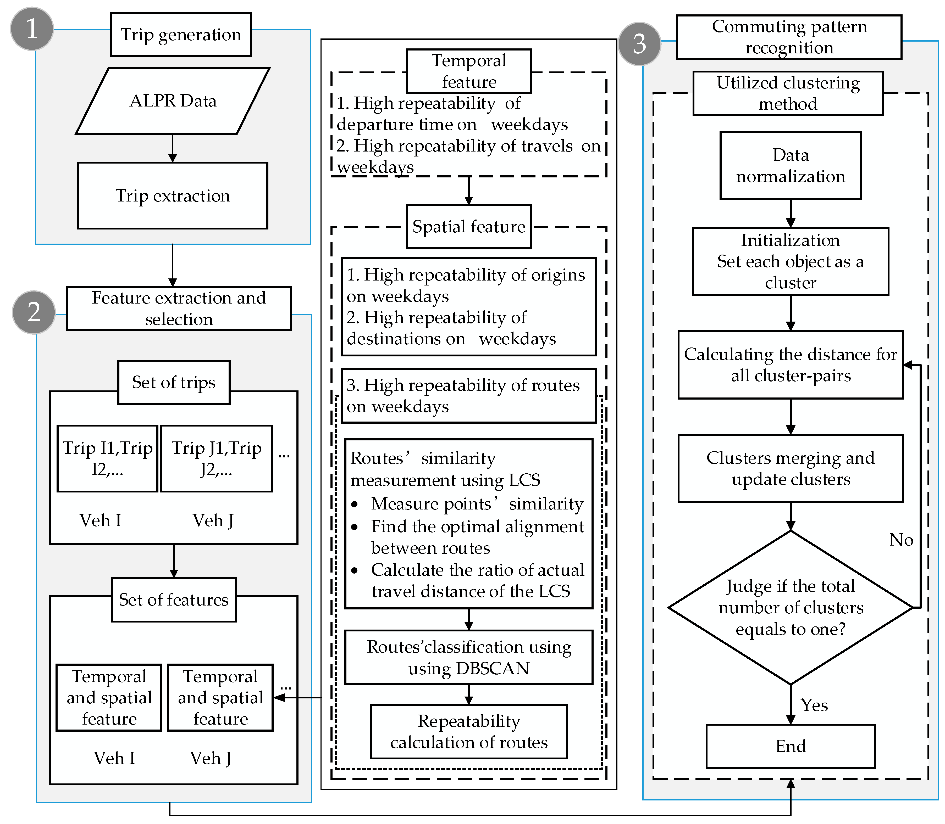
To investigate the commuting pattern of urban traffic, a systematic framework for commuting pattern recognition was developed and shown in Figure 1. The framework consists of three modules: data preprocessing, feature extraction and selection, and commuting pattern recognition.

Figure 1. The systematic framework for commuting pattern recognition. “ALRP” means Automatic License Plate Recognition technology, “Veh” is a Vehicle, “LCS” means the Longest Common Subsequence method, “DBSCAN” is a clustering method named “Density-Based Spatial Clustering of Applications with Noise”.

As shown in Figure 1, firstly, to analyze the travel behavior of a single vehicle the trips of each vehicle were extracted from ALPR data in a module using a trajectory reconstruction method [25]. Secondly, considering the repeatability of commuting vehicles, the temporal and spatial features were both extracted and selected through commuting activities analysis, specifically, the route feature was derived using the LCS (Longest Common Subsequence) method. The LCS aims to find the longest subsequence common to all sequences in a set of sequences, it can be used to classify vehicle trajectories. Thirdly, the selected features of vehicles were utilized by a hierarchical clustering method to identify the commuting vehicles.

2.1. Trip Generation from ALPR Data

Trip generation is an important basis for commuting pattern recognition using ALPR data. A trip is composed of a sequence of activities for a particular purpose [29]. To generate trips with ALPR data the license matching method is utilized. Briefly, a vehicle’s trajectory is formed by a group of time-ordered ALPR devices that captured the vehicles. The trips are generated by analyzing the activities of the traveler.

Generally, the travel time of a vehicle between two intersections must be in a certain range. If the vehicle’s travel time between two adjacent intersections is far beyond the range, the vehicle’s trajectory can be referred to as two different trips. Based on this, a time threshold [20] is utilized to segregate the trajectory into multiple trips. With generated trips, the origins and destinations can be easily derived. It is worth mentioning that, as the ALPR devices are installed at intersections, the actual origin and destination of trips may not be captured. Therefore, the first and the last records of each trip are approximately regarded as the trip’s origin and destination, respectively [20]. The recorded time of the first and last record of each trip can be viewed as the trip’s departure time and arrival time.

2.2. Feature Selection and Extraction

To identify the commuting pattern of an urban road network, the commuters and non-commuters are distinguished with different travel behaviors using ALPR data. Generally, the commuting travelers are likely to go off for work/home regularly with relatively fixed locations at similar times. Specifically, commuters’ behavior has two features: (1) High repeatability during the same duration (e.g., morning peak) on weekdays; (2) high repeatability of origin and destination (e.g., family, workplace) on weekdays. Therefore, the features of a commuting vehicle can be temporally and spatially measured.

The temporal features of a traveler could be departure time, arrival time, travel time and the number of travelling weekdays. Affected by travel distance and traffic conditions, the arrival time and travel time have large uncertainty and thus cannot be used for exploring the temporal pattern. As commuters tend to travel at morning and evening peaks on weekdays, the departure time and the number of travelling weekdays are used to describe the temporal features of a traveler. It is obvious that the higher occurrence at evening/morning peaks is more likely to signal that the traveler is a commuter.

To quantify the temporal feature of a traveler, the vehicles that appear both at morning and evening peaks of weekdays are extracted. Then, the number of days these vehicles appear is calculated as Equation (1).

$${\mathrm{N}}_{\mathrm{d}}^{\mathrm{i}}={\sum }_{\mathrm{k}=1}^{\mathrm{D}}{\mathrm{n}}_{\mathrm{k}}^{\mathrm{i}},{\mathrm{n}}_{\mathrm{k}}^{\mathrm{i}}=(0\mathrm{or}1)$$

(1)

where ${\mathrm{N}}_{\mathrm{d}}^{\mathrm{i}}$ is the number of days that a vehicle appears at weekday peaks, $\mathrm{D}$ is the total number of studied days. ${\mathrm{n}}_{\mathrm{k}}^{\mathrm{i}}=1$ means that vehicle $\mathrm{i}$ appears both at the morning peak and the evening peak on the k-th weekday.

The spatial features of a traveler can be expressed as the repeatability of origins and destinations as well as the selected routes. To improve the reliability of commuting trip recognition, the three features were all utilized. Generally, the origin and destination of a commuter are relatively stable on weekdays. Therefore, the higher repeatability of origins and destinations, the more likely the traveler is a commuter. Specifically, the first trip and the last trip on a weekday were considered as a home-to-work trip and a work-to-home trip, respectively. The origin of the first trip of a vehicle for a weekday was defined as a traveler’s origin (TrO), and the origin of the last trip for a weekday was defined as a traveler’s destination (TrD). The repeatability of origins and destinations of a traveler were quantified by the number of unique TrOs and TrDs on the studied weekdays which are shown as Equation (2).

$$\begin{gathered} {\mathrm{N}}_s^{\mathrm{i}}=\mathrm{length}({\mathrm{O}}^{\mathrm{i}}), \\ {\mathrm{O}}^{\mathrm{i}}=\mathrm{unique}({\mathrm{A}}^{\mathrm{i}}),{\mathrm{A}}^{\mathrm{i}}={\mathrm{o}}_1^{\mathrm{i}},{\mathrm{o}}_{\mathrm{k}}^{\mathrm{i}}\dots {\mathrm{o}}_{\mathrm{w}}^{\mathrm{i}}, \\ {\mathrm{N}}_{\mathrm{e}}^{\mathrm{i}}=\mathrm{length}({\mathrm{D}}^{\mathrm{i}}), \\ {\mathrm{D}}^{\mathrm{i}}=\mathrm{unique}({\mathrm{B}}^{\mathrm{i}}),{\mathrm{B}}^{\mathrm{i}}={\mathrm{d}}_1^{\mathrm{i}},{\mathrm{d}}_{\mathrm{k}}^{\mathrm{i}}\dots {\mathrm{d}}_{\mathrm{w}}^{\mathrm{i}}. \end{gathered}$$

(2)

where ${\mathrm{o}}_{\mathrm{k}}^{\mathrm{i}}$ and ${\mathrm{d}}_{\mathrm{k}}^{\mathrm{i}}$ are the TrO and TrD of vehicle $\mathrm{i}$ on the kth weekday. ${\mathrm{A}}^{\mathrm{i}}$ and ${\mathrm{B}}^{\mathrm{i}}$ are noted the collections of TrO and TrD for multiple weekdays, individually. ${\mathrm{O}}^{\mathrm{i}}$ and ${\mathrm{D}}^{\mathrm{i}}$ are the collections of different origins and destinations in ${\mathrm{A}}^{\mathrm{i}}$ and ${\mathrm{B}}^{\mathrm{i}}$, respectively. ${\mathrm{N}}_{\mathrm{s}}^{\mathrm{i}}$ and ${\mathrm{N}}_{\mathrm{e}}^{\mathrm{i}}$ are the numbers of different origins and destinations in ${\mathrm{O}}^{\mathrm{i}}$ and ${\mathrm{D}}^{\mathrm{i}}$, individually. “Unique” is a function for enumerating the different entities in an array, “length” is an function for getting the number of entities in an array.

The third spatial feature of a traveler is the repeatability of routes ${\mathrm{N}}_{\mathrm{r}}^{\mathrm{i}}$. Commuters are inclined to choose several familiar routes to ensure the reliability of travelling; these routes are called frequently used routes (FURs). It was assumed that the FURs of a commuter were the ones with high repeatability in multiple weekdays, and any route can be classified as one of the FURs. The FURs may vary with different considerations, for example, a commuter may select a route with relative short distance or travel time. However, the number of FURs should be fixed to a small value. The repeatability of the selected routes of a traveler was derived with following steps. First, the similarity between different routes on multiple weekdays was measured with the Longest Common Subsequence (LCS). Second, the selected routes for multiple days were classified into several groups using the DBSCAN (Density-Based Spatial Clustering of Applications with Noise) method, which is a density-based non-parametric clustering algorithm. Then the FURs were included in one or more groups. Last, for the groups including FURs, the smaller averaged within-cluster distance, the more likely the traveler was a commuter. For the groups without FURs, the fewer number of routes, the more likely the traveler was a commuter.

To quantify the similarity between different selected routes, the Longest Common Subsequence (LCS) was utilized [30]. The LCS aims to find the longest common subsequence of two sequences. To derive the LCS for two routes, first, the similarity measurement method for two points of two different routes was defined. Second, the optimal alignment was determined through establishing the correspondence of the two routes’ points. Finally, the ratio of the actual travel distance of the LCS was calculated. Specifically, a route was formed by a series of connected intersections, and the intersections were abstracted as points, which is described as Equation (3).

$${\mathrm{r}}_{\mathrm{A}}^{\mathrm{Ik}}=({\mathrm{s}}_1,{\mathrm{s}}_2,{\mathrm{s}}_{\mathrm{i}}\dots ,{\mathrm{s}}_{\mathrm{m}},\dots {\mathrm{s}}_{\mathrm{M}}),{\mathrm{r}}_{\mathrm{B}}^{\mathrm{Ik}}=({\mathrm{s}}_1,{\mathrm{s}}_2,{\mathrm{s}}_{\mathrm{j}}\dots {\mathrm{s}}_{\mathrm{n}},\dots {\mathrm{s}}_{\mathrm{N}}),$$

(3)

where ${\mathrm{r}}_{\mathrm{A}}^{\mathrm{Ik}}$, ${\mathrm{r}}_{\mathrm{B}}^{\mathrm{Ik}}$ are route $\mathrm{A}$ and route $\mathrm{B}$ of vehicle $\mathrm{I}$ on the $\mathrm{k}$ th weekday with size $\mathrm{M}$ and $\mathrm{N}$, ${\mathrm{s}}_{\mathrm{i}}$, ${\mathrm{s}}_{\mathrm{j}}$ are the $\mathrm{i}$ th and $\mathrm{j}$ th point of ${\mathrm{r}}_{\mathrm{A}}^{\mathrm{Ik}}$ and ${\mathrm{r}}_{\mathrm{B}}^{\mathrm{Ik}}$.

To measure the similarity of two points in two different routes, the approximation degree of spatial location of the two points ($\mathrm{simP}({\mathrm{s}}_{\mathrm{i}},{\mathrm{s}}_{\mathrm{j}})$) was utilized. The specific formulas are expressed in Equation (4).

$$\mathrm{simP}({\mathrm{s}}_{\mathrm{i}},{\mathrm{s}}_{\mathrm{j}})=\{\begin{array}{c}0,\mathrm{if}\mathrm{dis}({\mathrm{s}}_{\mathrm{i}},{\mathrm{s}}_{\mathrm{j}})>\mathsf{\gamma }\\ 1-\frac{\mathrm{dis}({\mathrm{s}}_{\mathrm{i}},{\mathrm{s}}_{\mathrm{j}})}{\mathsf{\gamma }},\mathrm{otherwise}\end{array}$$

(4)

where $\mathrm{dis}({\mathrm{s}}_{\mathrm{i}},{\mathrm{s}}_{\mathrm{j}})$ is the Euclidean distance derived from the geographical coordinates of the two points. $\mathsf{\gamma }$ is the allowable maximum distance. The two points are matched when $\mathrm{simP}({\mathrm{s}}_{\mathrm{i}},{\mathrm{s}}_{\mathrm{j}})>0$.

To find the optional alignment between two routes, a dynamic programing algorithm was utilized [30]. The optional alignment was derived through maximizing the accumulated similarity of the matched points. The cumulative similarity can be calculated as Equation (5).

$$\mathsf{\beta }({\mathrm{r}}_{\mathrm{A}(\mathrm{m})}^{\mathrm{Ik}},{\mathrm{r}}_{\mathrm{B}(\mathrm{n})}^{\mathrm{Ik}})=\max \{(\mathrm{simP}({\mathrm{s}}_{\mathrm{m}},{\mathrm{s}}_{\mathrm{n}})+\mathsf{\beta }({\mathrm{r}}_{\mathrm{A}(\mathrm{m}-1)}^{\mathrm{Ik}},{\mathrm{r}}_{\mathrm{B}(\mathrm{n}-1)}^{\mathrm{Ik}})),\mathsf{\beta }({\mathrm{r}}_{\mathrm{A}(\mathrm{m})}^{\mathrm{Ik}},{\mathrm{r}}_{\mathrm{B}(\mathrm{n}-1)}^{\mathrm{Ik}}),\mathsf{\beta }({\mathrm{r}}_{\mathrm{A}(\mathrm{m}-1)}^{\mathrm{Ik}},{\mathrm{r}}_{\mathrm{B}(\mathrm{n})}^{\mathrm{Ik}})\}$$

(5)

where ${\mathrm{r}}_{\mathrm{A}(\mathrm{m})}^{\mathrm{Ik}}$, ${\mathrm{r}}_{\mathrm{B}(\mathrm{n})}^{\mathrm{Ik}}$ are the first $\mathrm{m}$ and $\mathrm{n}$ points of route ${\mathrm{r}}_{\mathrm{A}}^{\mathrm{Ik}}$ and ${\mathrm{r}}_{\mathrm{B}}^{\mathrm{Ik}}$, respectively. ${\mathsf{\beta }(\mathrm{r}}_{\mathrm{A}(\mathrm{m})}^{\mathrm{Ik}},{\mathrm{r}}_{\mathrm{B}(\mathrm{n})}^{\mathrm{Ik}})$ is the cumulative similarity of the matched points under the optimal alignment between ${\mathrm{r}}_{\mathrm{A}(\mathrm{m})}^{\mathrm{Ik}}$ and ${\mathrm{r}}_{\mathrm{B}(\mathrm{n})}^{\mathrm{Ik}}$, $\mathsf{\beta }({\mathrm{r}}_{\mathrm{A}(\mathrm{m})}^{\mathrm{Ik}},{\mathrm{r}}_{\mathrm{B}(\mathrm{n})}^{\mathrm{Ik}})=0,\mathrm{if}\mathrm{n}=0\mathrm{or}\mathrm{m}=0$. ${\mathsf{\beta }(\mathrm{r}}_{\mathrm{A}(\mathrm{m})}^{\mathrm{Ik}},{\mathrm{r}}_{\mathrm{B}(\mathrm{n})}^{\mathrm{Ik}})$ is derived through literately calculating ${\mathrm{r}}_{\mathrm{A}(\mathrm{m}-1)}^{\mathrm{Ik}},{\mathrm{r}}_{\mathrm{B}(\mathrm{n}-1)}^{\mathrm{Ik}}$, $\mathrm{simP}({\mathrm{s}}_{\mathrm{m}},{\mathrm{s}}_{\mathrm{n}})$, $\mathsf{\beta }({\mathrm{r}}_{\mathrm{A}(\mathrm{m})}^{\mathrm{Ik}},{\mathrm{r}}_{\mathrm{B}(\mathrm{n}-1)}^{\mathrm{Ik}})$ and $\mathsf{\beta }({\mathrm{r}}_{\mathrm{A}(\mathrm{m}-1)}^{\mathrm{Ik}},{\mathrm{r}}_{\mathrm{B}(\mathrm{n})}^{\mathrm{Ik}})$. The correspondence between points of the two routes for optional alignment was established through keeping track of the matched points which contributed to the final cumulative similarity ${\mathsf{\beta }(\mathrm{r}}_{\mathrm{A}(\mathrm{M})}^{\mathrm{Ik}},{\mathrm{r}}_{\mathrm{B}(\mathrm{N})}^{\mathrm{Ik}})$. Based on this, the LCS was determined by the consecutive points with the largest number. As the accumulated similarity between each pair of points of the two routes was calculated only once, the algorithm’s time complexity was $\mathrm{O}(\mathrm{M}\times \mathrm{N})$, where M and N are the number of points of the two routes, respectively.

With the LCS identified, the similarity between the two routes was measured with the ratio of the actual travel distance of the LCS. Specifically, the actual travel distance of LCS was derived by summing all the distance derived from the geographical coordinates of the consecutive points in LCS, which is described as $\mathrm{len}({\mathrm{L}}_{(\mathrm{i},\mathrm{j})})={\sum }_{\mathrm{x}=1}^{\mathrm{X}-1}\mathrm{dis}({\mathrm{L}}_{\mathrm{x}},{\mathrm{L}}_{\mathrm{x}+1})$, where $\mathrm{X}$ is the number of matches, ${\mathrm{L}}_{(\mathrm{i},\mathrm{j})}=({\mathrm{L}}_1,\dots ,{\mathrm{L}}_{\mathrm{X}})$ is the derived LCS for route ${\mathrm{r}}_{\mathrm{A}}^{\mathrm{Ik}}$ and ${\mathrm{r}}_{\mathrm{B}}^{\mathrm{Ik}}$, ${\mathrm{L}}_1,\dots ,{\mathrm{L}}_{\mathrm{X}}$ are the matched points. As the matched points are approximate, the LCS can be extracted either from route ${\mathrm{r}}_{\mathrm{A}}^{\mathrm{Ik}}$ or ${\mathrm{r}}_{\mathrm{B}}^{\mathrm{Ik}}$. The LCS for the two routes are described as ${\mathrm{L}}_{(\mathrm{i},\mathrm{j})}{}^{\mathrm{A}}$ and ${\mathrm{L}}_{(\mathrm{i},\mathrm{j})}{}^{\mathrm{B}}$, respectively. Based on this, the similarity of ${\mathrm{r}}_{\mathrm{A}}^{\mathrm{Ik}}$ and ${\mathrm{r}}_{\mathrm{B}}^{\mathrm{Ik}}$ was derived by calculating the ratio of $\mathrm{len}({\mathrm{L}}_{(\mathrm{i},\mathrm{j})})$ in the route with shorter distance which is shown in Equation (6).

$$\mathrm{simR}({\mathrm{r}}_{\mathrm{A}}^{\mathrm{Ik}},{\mathrm{r}}_{\mathrm{B}}^{\mathrm{Ik}})=\{\begin{array}{ll}& 0\mathrm{if}\min \left(\mathrm{len}\left({\mathrm{L}}_{\left(\mathrm{i},\mathrm{j}\right)}{}^{\mathrm{A}}\right)\mathrm{len}\left({\mathrm{L}}_{\left(\mathrm{i},\mathrm{j}\right)}{}^{\mathrm{B}}\right)\right)<\mathsf{\delta }\\ & \frac{\mathrm{len}\left({\mathrm{L}}_{\left(\mathrm{i},\mathrm{j}\right)}{}^{\mathrm{A}}\right)}{\mathrm{len}\left({\mathrm{r}}_{\mathrm{A}}^{\mathrm{Ik}}\right)}\hspace{1em}\mathrm{if}\mathrm{len}({\mathrm{r}}_{\mathrm{A}}^{\mathrm{Ik}})<\mathrm{len}\left({\mathrm{r}}_{\mathrm{B}}^{\mathrm{Ik}}\right)\\ & \frac{\mathrm{len}\left({\mathrm{L}}_{\left(\mathrm{i},\mathrm{j}\right)}{}^{\mathrm{B}}\right)}{\mathrm{len}\left({\mathrm{r}}_{\mathrm{B}}^{\mathrm{Ik}}\right)}\hspace{1em}\mathrm{if}\mathrm{len}\left({\mathrm{r}}_{\mathrm{A}}^{\mathrm{Ik}}\right)>\mathrm{len}\left({\mathrm{r}}_{\mathrm{B}}^{\mathrm{Ik}}\right)\end{array}$$

(6)

where $\mathsf{\delta }$ is the allowable minimum length for a valid LCS between two routes; $\mathrm{simR}({\mathrm{r}}_{\mathrm{A}}^{\mathrm{Ik}},{\mathrm{r}}_{\mathrm{B}}^{\mathrm{Ik}})$ represents the similarity between route ${\mathrm{r}}_{\mathrm{A}}^{\mathrm{Ik}}$ and ${\mathrm{r}}_{\mathrm{B}}^{\mathrm{Ik}}$.

With the similarity value ($\mathrm{simR}$) between different routes, a DBSCAN clustering method was then used to classify the routes. The details of the DBSCAN method can be find in our previous study [17]. The repeatability of selected routes of a traveler was quantified as ${\mathrm{N}}_{\mathrm{r}}^{\mathrm{i}}$, and the calculation for ${\mathrm{N}}_{\mathrm{r}}^{\mathrm{i}}$ is shown in Equation (7).

$$\begin{gathered} {\mathrm{N}}_{\mathrm{r}}^{\mathrm{i}}=1-({\mathrm{distC}}_{\mathrm{FUR}}/{\mathrm{k}}_{\mathrm{FUR}}+\mathrm{N}({\mathrm{C}}_{\mathrm{non-FUR}})) \\ {\mathrm{distC}}_{\mathrm{FUR}}=({\displaystyle \sum }_{\mathrm{j}=1}^{{\mathrm{k}}_{\mathrm{FUR}}}{\displaystyle \sum }_{\mathrm{simR}(\mathrm{j})\in {\mathrm{C}}_{\mathrm{j}}}||\mathrm{simR}(\mathrm{j})-{\mathrm{c}}_{\mathrm{j}}||{}^2{)/\mathrm{k}}_{\mathrm{FUR}} \end{gathered}$$

(7)

where ${\mathrm{distC}}_{\mathrm{FUR}}$ represents the averaged within-cluster distance for clusters with FURs, $\mathrm{N}({\mathrm{C}}_{\mathrm{non-FUR}})$ is the number of routes within the clusters without FURs, ${\mathrm{k}}_{\mathrm{FUR}}$ represents the number of clusters with FURs, ${\mathrm{C}}_{\mathrm{j}}$ is the j-th cluster, ${\mathrm{c}}_{\mathrm{j}}$ is the centroid of cluster ${\mathrm{C}}_{\mathrm{j}}$, $\left|\right|\mathrm{simR}(\mathrm{j})-{\mathrm{c}}_{\mathrm{j}}\left|\right|$ is the L2 norm (Euclidean distance) between the two vectors, and $\mathrm{simR}(\mathrm{j})$ is a data point in ${\mathrm{C}}_{\mathrm{j}}$. It is worth noting that to make the parameters comparable, the $\mathrm{simR}(\mathrm{j})$ and $\mathrm{N}({\mathrm{C}}_{\mathrm{non-FUR}})$ were scaled. Obviously, the higher the value of ${\mathrm{N}}_{\mathrm{r}}^{\mathrm{i}}$, the more likely the traveler was a commuter.

2.3. Commuting Vehicles Identification Using Ward’s Hierarchical Clustering

To identify the commuting vehicles, a clustering technique was utilized to analyze temporal-spatial features extracted from ALPR data. Many clustering algorithms and strategies, such as K-means [24,31], DBSCAN [32], GMM (Gaussian Mixture Model) [33], nested clustering [34], online agglomerative clustering [35], hierarchical clustering [36], and other algorithms [37,38] had been proposed in the past decades. Hierarchical clustering, as a typical unsupervised machine learning algorithm, has been applied to a wide spectrum of transportation researches. Since the Ward’s hierarchical clustering (Hclust) [36] method does not need an initial number of clusters and initial composition rules and has the advantage of possessing easily computable extended dissimilarity indices [39], it was utilized to extract the commuting vehicles in our study. Due to the computational complexity of merging at each step for the large dataset, the Lance-Williams algorithm [36] was utilized to improve the computing efficiency. A suitable number of clusters were selected using the hierarchy (which is also known as “dendrogram”) from successive merging. The details of the Hclust method are as follows:

The features extracted from all vehicles are included in dataset $\mathrm{C}$. $\mathrm{C}=\{{\mathrm{P}}_1,{\mathrm{P}}_2,\dots ,{\mathrm{P}}_{\mathrm{i}},\dots ,{\mathrm{P}}_{\mathrm{j}},\dots ,{\mathrm{P}}_{\mathrm{m}}\}$. ${\mathrm{P}}_{\mathrm{i}}$ and ${\mathrm{P}}_{\mathrm{j}}$ are the $\mathrm{i}$ th and $\mathrm{j}$ th vehicle’s feature in $\mathrm{C}$, $\mathrm{m}$ is the total number of vehicles. Vehicle ${\mathrm{P}}_{\mathrm{i}}$ has four features ${\mathrm{P}}_{\mathrm{i}}=({\mathrm{N}}_{\mathrm{d}}^{\mathrm{i}},{\mathrm{N}}_{\mathrm{s}}^{\mathrm{i}},{\mathrm{N}}_{\mathrm{e}}^{\mathrm{i}},{\mathrm{N}}_{\mathrm{r}}^{\mathrm{i}})$, specifically, ${\mathrm{N}}_{\mathrm{d}}^{\mathrm{i}}$ is the number of days that a vehicle appears at weekday peaks, ${\mathrm{N}}_{\mathrm{s}}^{\mathrm{i}}$ and ${\mathrm{N}}_{\mathrm{e}}^{\mathrm{i}}$ are the numbers of different origins and destinations, ${\mathrm{N}}_{\mathrm{r}}^{\mathrm{i}}$ denotes the repeatability of selected routes of a traveler. It is noted that the variables have rescaled before calculating the distance. The Hclust algorithm consists of two parts: the objection function and dissimilarity measurement.

2.3.1. Objective Function

The objective of the Hclust algorithm is to minimize the increase of total within-cluster variance at each iteration until all clusters are merged into one. In other words, the objective of the Hclust algorithm is to find a pair of clusters with minimum distance among all pairwise distances at each step. Take the first iteration as an example to initialize the algorithm, set each object ${\mathrm{P}}_{\mathrm{i}}$ and ${\mathrm{P}}_{\mathrm{j}}$ as cluster ${\mathrm{C}}_{{\mathrm{P}}_{\mathrm{i}}}$ and ${\mathrm{C}}_{{\mathrm{P}}_{\mathrm{j}}}$, individually. The dissimilarities between ${\mathrm{C}}_{{\mathrm{P}}_{\mathrm{i}}}$ and ${\mathrm{C}}_{{\mathrm{P}}_{\mathrm{j}}}$ is noted as ${\mathrm{d}}_{{(\mathrm{P}}_{\mathrm{i}}{)(\mathrm{P}}_{\mathrm{j}})}$. The total number of vehicles to be clustered is $\mathrm{m}$, the objective function $\mathrm{J}$ for the first iteration is described in Equation (8):

$$\mathrm{J}=\min {\mathrm{d}}_{(\mathrm{P}\mathrm{i})(\mathrm{P}\mathrm{j})},1\le \mathrm{i},\mathrm{j}\le \mathrm{m},\mathrm{i}\ne \mathrm{j}$$

(8)

2.3.2. Dissimilarity Measurement

With the agglomeration of vehicles’ features, there are two kinds of data to be classified: a single feature and a combination of features. The combination of features may be formed by many clusters. To determine the pair of clusters with minimum distance, the distance between feature to feature (Euclidean distance), feature to the combination of features (intra-cluster distance), and the combination of features to the combination of features (global cluster distance) should be calculated. In brief, two kinds of dissimilarity, the intra-cluster and global cluster dissimilarity, are measured between different clusters. Assume that ${\mathrm{C}}_{{\mathrm{P}}_{\mathrm{i}}}$ and ${\mathrm{C}}_{{\mathrm{P}}_{\mathrm{j}}}$ are included in clusters ${\mathrm{C}}_{\mathrm{i}}$ and ${\mathrm{C}}_{\mathrm{j}}$, and ${\mathrm{C}}_{\mathrm{i}}$ and ${\mathrm{C}}_{\mathrm{j}}$ have the minimum distances during $\mathrm{t}$-th iteration. Then ${\mathrm{C}}_{\mathrm{i}}$ and ${\mathrm{C}}_{\mathrm{j}}$ are merged as ${\mathrm{C}}_{\mathrm{i}\cup \mathrm{j}}$ in the $(\mathrm{t}+1)$-th iteration. After $(\mathrm{t}+1)$ th iteration, assume that there is a cluster ${\mathrm{C}}_{\mathrm{k}}$ in $\mathrm{C}$, if ${\mathrm{C}}_{\mathrm{i}\cup \mathrm{j}}$ and ${\mathrm{C}}_{\mathrm{k}}$ have the minimum distance, then ${\mathrm{C}}_{\mathrm{i}\cup \mathrm{j}}$ and ${\mathrm{C}}_{\mathrm{k}}$ can be merged in the next iteration. Given that the dissimilarities between ${\mathrm{C}}_{\mathrm{i}}$ and ${\mathrm{C}}_{\mathrm{j}}$ are noted as ${\mathrm{d}}_{\mathrm{ij}}$, the intra-cluster dissimilarity between cluster ${\mathrm{C}}_{\mathrm{i}\cup \mathrm{j}}$ and ${\mathrm{C}}_{\mathrm{k}}$ can be expressed as Equations (9) and (10):

$${\mathrm{d}}_{(\mathrm{ij})\mathrm{k}}={\mathsf{\alpha }}_{\mathrm{i}}{\mathrm{d}}_{\mathrm{ik}}+{\mathsf{\alpha }}_{\mathrm{j}}{\mathrm{d}}_{\mathrm{jk}}+\mathsf{\beta }{\mathrm{d}}_{\mathrm{ij}}$$

(9)

$${\mathsf{\alpha }}_{\mathrm{i}}=\frac{{\mathrm{n}}_{\mathrm{i}}+{\mathrm{n}}_{\mathrm{k}}}{{\mathrm{n}}_{\mathrm{i}}+{\mathrm{n}}_{\mathrm{j}}+{\mathrm{n}}_{\mathrm{k}}},{\mathsf{\alpha }}_{\mathrm{j}}=\frac{{\mathrm{n}}_{\mathrm{j}}+{\mathrm{n}}_{\mathrm{k}}}{{\mathrm{n}}_{\mathrm{i}}+{\mathrm{n}}_{\mathrm{j}}+{\mathrm{n}}_{\mathrm{k}}},\mathsf{\beta }=\frac{-{\mathrm{n}}_{\mathrm{k}}}{{\mathrm{n}}_{\mathrm{i}}+{\mathrm{n}}_{\mathrm{j}}+{\mathrm{n}}_{\mathrm{k}}}$$

(10)

where ${\mathrm{d}}_{\mathrm{ij}},{\mathrm{d}}_{\mathrm{ik}}$ and ${\mathrm{d}}_{\mathrm{jk}}$ are the pair-wise distances between clusters ${\mathrm{C}}_{\mathrm{i}}$, ${\mathrm{C}}_{\mathrm{j}}$ and ${\mathrm{C}}_{\mathrm{k}}$, respectively. ${\mathrm{d}}_{(\mathrm{ij})\mathrm{k}}$ is the distance between the clusters ${\mathrm{C}}_{\mathrm{i}\cup \mathrm{j}}$ and ${\mathrm{C}}_{\mathrm{k}}$. ${\mathrm{n}}_{\mathrm{i}}$, ${\mathrm{n}}_{\mathrm{j}}$ and ${\mathrm{n}}_{\mathrm{k}}$ represent the size of cluster ${\mathrm{C}}_{\mathrm{i}},{\mathrm{C}}_{\mathrm{j}}$ and ${\mathrm{C}}_{\mathrm{k}}$, respectively. ${\mathsf{\alpha }}_{\mathrm{i}}$, ${\mathsf{\alpha }}_{\mathrm{j}}$ and $\mathsf{\beta }$ in Equations (9) and (10) illustrate that the distance between ${\mathrm{C}}_{\mathrm{i}\cup \mathrm{j}}$ and ${\mathrm{C}}_{\mathrm{k}}$ is related to the size of each cluster.

The global cluster dissimilarity can be described as Equation (11):

$${\mathrm{d}}_{\mathrm{AB}}=\sqrt{\frac{2{\mathrm{n}}_{\mathrm{A}}\times {\mathrm{n}}_{\mathrm{B}}}{{\mathrm{n}}_{\mathrm{A}}+{\mathrm{n}}_{\mathrm{B}}}}\times ||\overrightarrow{{\mathrm{c}}_{\mathrm{A}}}-\overrightarrow{{\mathrm{c}}_{\mathrm{B}}}||$$

(11)

where ${\mathrm{d}}_{\mathrm{AB}}$ is the weighted Euclidean distance between the centroids of cluster ${\mathrm{C}}_{\mathrm{A}}$ and ${\mathrm{C}}_{\mathrm{B}}$, $\overrightarrow{{\mathrm{c}}_{\mathrm{A}}}$ and $\overrightarrow{{\mathrm{c}}_{\mathrm{B}}}$ are the averaged vector of cluster ${\mathrm{C}}_{\mathrm{A}}$ and ${\mathrm{C}}_{\mathrm{B}}$, which represent the centroids of the points in cluster ${\mathrm{C}}_{\mathrm{A}}$ and ${\mathrm{C}}_{\mathrm{B}}$, respectively. $\left|\right|\left|\right|$ is the operation of calculating the Euclidean distance. When the cluster-pairs both are formed by a single object, the dissimilarity is equals to the Euclidean distance between them.

2.3.3. Clustering Procedure

Let $\mathrm{C}={\mathrm{C}}_1,\dots {\mathrm{C}}_{\mathrm{m}}$ be the sets of clusters. The procedure of Ward’s hierarchical clustering method is shown in module 3 of Figure 1 and the main steps are summarized as follows:

Step 1: Initialization. Set each object (${\mathrm{P}}_{\mathrm{i}}$) as a cluster. ${\mathrm{C}}_{{\mathrm{P}}_{\mathrm{i}}}=\left\{{\mathrm{P}}_{\mathrm{i}}\right\}$, ${\mathrm{C}}_{{\mathrm{P}}_{\mathrm{j}}}=\left\{{\mathrm{P}}_{\mathrm{j}}\right\}$.

Step 2: Calculate the distance for all cluster-pairs using Equations (9)–(11).

Step 3: Clusters merging. Find a cluster-pairs ${\mathrm{C}}_{\mathrm{i}},{\mathrm{C}}_{\mathrm{j}}$ with the minimum distances and merge them into a new cluster ${\mathrm{C}}_{\mathrm{i}\cup \mathrm{j}}$. Then, add ${\mathrm{C}}_{\mathrm{i}\cup \mathrm{j}}$ to $\mathrm{C}$, remove ${\mathrm{C}}_{\mathrm{i}}$ and ${\mathrm{C}}_{\mathrm{i}}$ from C.

Step 4: Check the condition whether iteration terminates. Check if the total number of clusters in $\mathrm{C}$ is equal to 1, if yes, then stop iteration; if not, go to Step 5.

Step 5: Repeat step 2, 3 and 4.

3. Implementation

3.1. Data Description and Feature Extraction

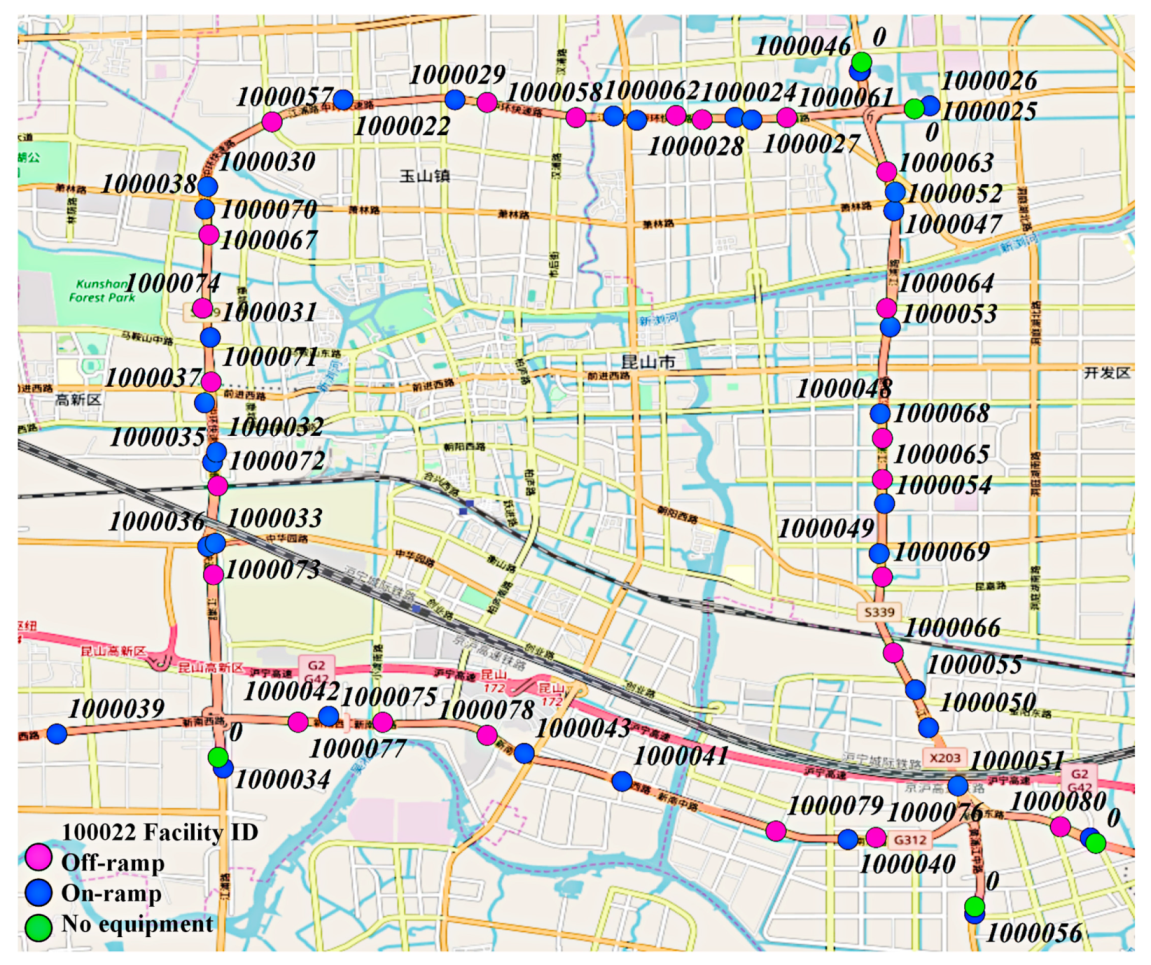
A ring expressway with 35 on-ramps and 24 off-ramps in Kunshan City, China was selected as the test site (as shown in Figure 2). As the selected network is a closed ring expressway network, the vehicle path can be determined by an origin and a destination. Therefore, only the origin and destination information were used to describe the spatial features of a traveler. The ALPR devices were located at on-ramps and off-ramps of the selected network.

Figure 2. The spatial distribution of the ramps of the test site.

The data was collected by 59 ALPR devices from 1–31 May 2017. A sample of raw data is shown in Table 1. The “TIME_KEY” consists of hour, minute, second and millisecond. For example, “92449840” means 09:24:49:840. “INSTALL_TYPE” represents the location of ALPR devices, “1” and “0” represent the devices installed at on-ramp and off-ramp, respectively. “LP_CAMERA_ID” is the ID of the ALPR devices. To protect travelers’ privacy, only the last four digits of the license number were displayed in the table.

Table 1. Examples of automatic license plate recognition (ALPR) data.

Date_Key	Time_Key	Week	License_Plate	Direc_tion	Install_Type	Lp_Camera_Id
20170501	92449840	Mon	…9603	WB	0	1000077
20170501	171139043	Mon	…0161	WB	1	1000049
20170501	171436975	Mon	…0161	WB	1	1000051
20170501	121404959	Mon	…0708	WB	1	1000048
20170501	123904031	Mon	…7HJ6	WB	1	1000043
20170501	201203163	Mon	…R8E8	WB	1	1000035
20170501	125711833	Mon	…SV31	WB	0	1000080

Note: “LP_CAMERA_ID” is the ID of the ALPR devices, “Mon” means Monday, ”WB” means westbound.

The data was pre-processed as follows: (1) To generate a vehicle trajectory, the “Lp_CAMERA_ID” were arranged together in time order; (2) a single trip was presented when the ordered neighboring records had different “INSTALL_TYPE” and the travel time was less than a threshold. In this study, the maximum travel time between two ALPR devices in test site is about 20 min, therefore, 20 min was set to be the time threshold; (3) the records with unidentified license plates were excluded; (4) given that the road network was totally-enclosed, any vehicle had to enter the network through the on-ramp and leave it through the off-ramp. The number of vehicles identified at on-ramps was viewed as the traffic demand ratio. With processed ALPR data, the extracted features were derived and a partial of which were shown in Table 2. Considering the higher temporal and spatial repeatability of a commuter, it was inferred that as the ID in Table 2 increases, the possibility of being a commuter decreased. To quantify the possibility and identify commuters, a clustering method was utilized in the following section.

Table 2. Examples of extracted features.

ID	License_Plate	${\mathit{N}}_{\mathit{d}}$	${\mathit{N}}_{\mathit{s}}$	${\mathit{N}}_{\mathit{e}}$
1	…F507	23	1	2
2	…K132	23	2	1
3	…5A58	22	3	4
4	…T8J3	19	4	1
5	…76PD	17	5	1
6	…303Q	17	1	5
7	…21S7	19	9	7
8	…0BA8	18	9	6
9	…H5N3	18	9	8
10	…5J23	12	9	7
11	…H3N1	13	8	9
12	…M80W	4	2	2

3.2. Performance Evaluation

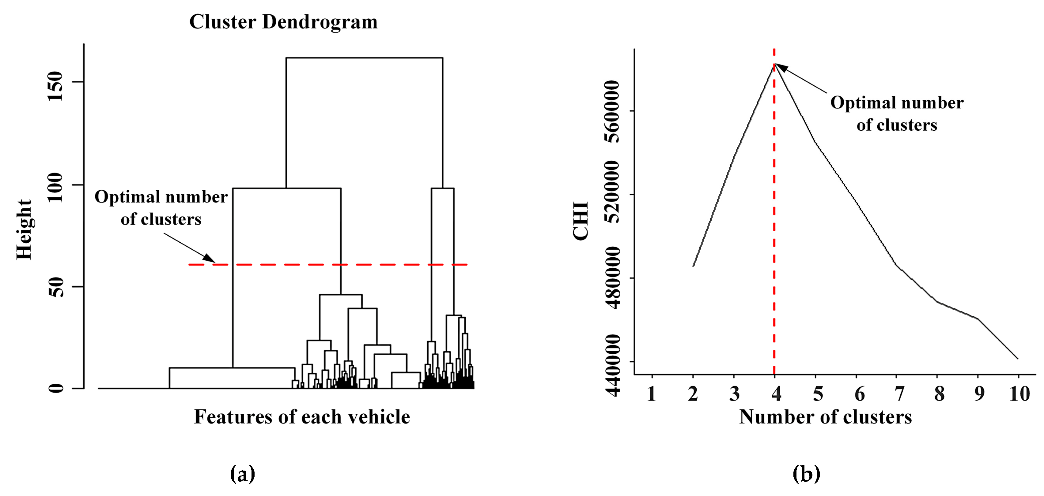
With extracted temporal and spatial features of commuting vehicles, the identification of commuting vehicles was implemented using the Hclust clustering method. To evaluate its performance, a comparison analysis was conducted between the Hclust method and the traditional clustering method, K-means. Before clustering, considering that the clustering results largely depends on the selection of the number of clusters, the dendrogram [40] (graphical structure) which revealed how the data objects merge into a single cluster and the Calinski-Harabasz Index ($\mathrm{CHI}$) [41] were utilized to determine the optimal number of clusters for the Hclust and K-means methods, respectively. Specifically, $\mathrm{CHI}$ evaluates the cluster validity based on the average between and within cluster sum of squares which are shown as Equations (12)–(14).

$$\mathrm{CHI}=({\mathrm{SS}}_{\mathrm{B}}/(\mathrm{K}-1))/({\mathrm{SS}}_{\mathrm{W}}/(\mathrm{m}-\mathrm{K}))$$

(12)

$${\mathrm{SS}}_{\mathrm{B}}={\displaystyle \sum }_{\mathrm{i}=1}^{\mathrm{k}}{\mathrm{m}}_{\mathrm{i}}{||{\mathrm{c}}_{\mathrm{i}}-\mathrm{c}||}^2$$

(13)

$${\mathrm{SS}}_{\mathrm{w}}={\displaystyle \sum }_{\mathrm{i}=1}^{\mathrm{k}}{\displaystyle \sum }_{{\mathrm{P}}_{\mathrm{i}}\in {\mathrm{C}}_{\mathrm{i}}}{||{\mathrm{P}}_{\mathrm{i}}-{\mathrm{c}}_{\mathrm{i}}||}^2$$

(14)

where ${\mathrm{SS}}_{\mathrm{w}}$ is the sum of squares within the clusters while ${\mathrm{SS}}_{\mathrm{B}}$ is the sum of squares among the clusters, $\mathrm{m}$ is the total number of data objects in the dataset, $\mathrm{c}$ is the dataset’s centroid, ${\mathrm{m}}_{\mathrm{i}}$ is the number of objects in ${\mathrm{C}}_{\mathrm{i}}$, $\mathrm{K}$ denotes the number of clusters, ${\mathrm{P}}_{\mathrm{i}}$ is the data point, ${\mathrm{C}}_{\mathrm{i}}$ is the i th cluster, ${\mathrm{c}}_{\mathrm{i}}$ is the centroid of cluster ${\mathrm{C}}_{\mathrm{i}}$, and $\left|\right|{\mathrm{P}}_{\mathrm{i}}-{\mathrm{c}}_{\mathrm{i}}\left|\right|$ is the L2 norm between the two vectors. The higher the value of $\mathrm{CHI}$, the more reasonable a cluster number is.

Figure 3a is the dendogram of extracted features (${\mathrm{N}}_{\mathrm{d}},{\mathrm{N}}_{\mathrm{s}},{\mathrm{N}}_{\mathrm{e}}$) based on the Hclust and it depicts the hierarchical relationship of 494,528 vehicle features. The dendrogram graphically displays the merging process and the intermediate clusters, and the graphical structure shows how points can be merged into a single cluster. The height of the dendogram implies the distance between the clusters. Based on the graphical interpretation of the dendrogram in Figure 3a, the optimal number of clusters could be two or four. The data structure with four clusters can be found by the horizontal line (red dotted line). Figure 3b is the $\mathrm{CHI}$ for K-means. It is obvious that the highest $\mathrm{CHI}$ (optimal) occurs when the number of clusters is four. Therefore, a four-cluster model was used in this study.

Figure 3. The determination for optimal number of clusters for the two methods. (a) The dendrogram using Hclust, (b) the CHI (Calinski-Harabasz Index) using K-means method.

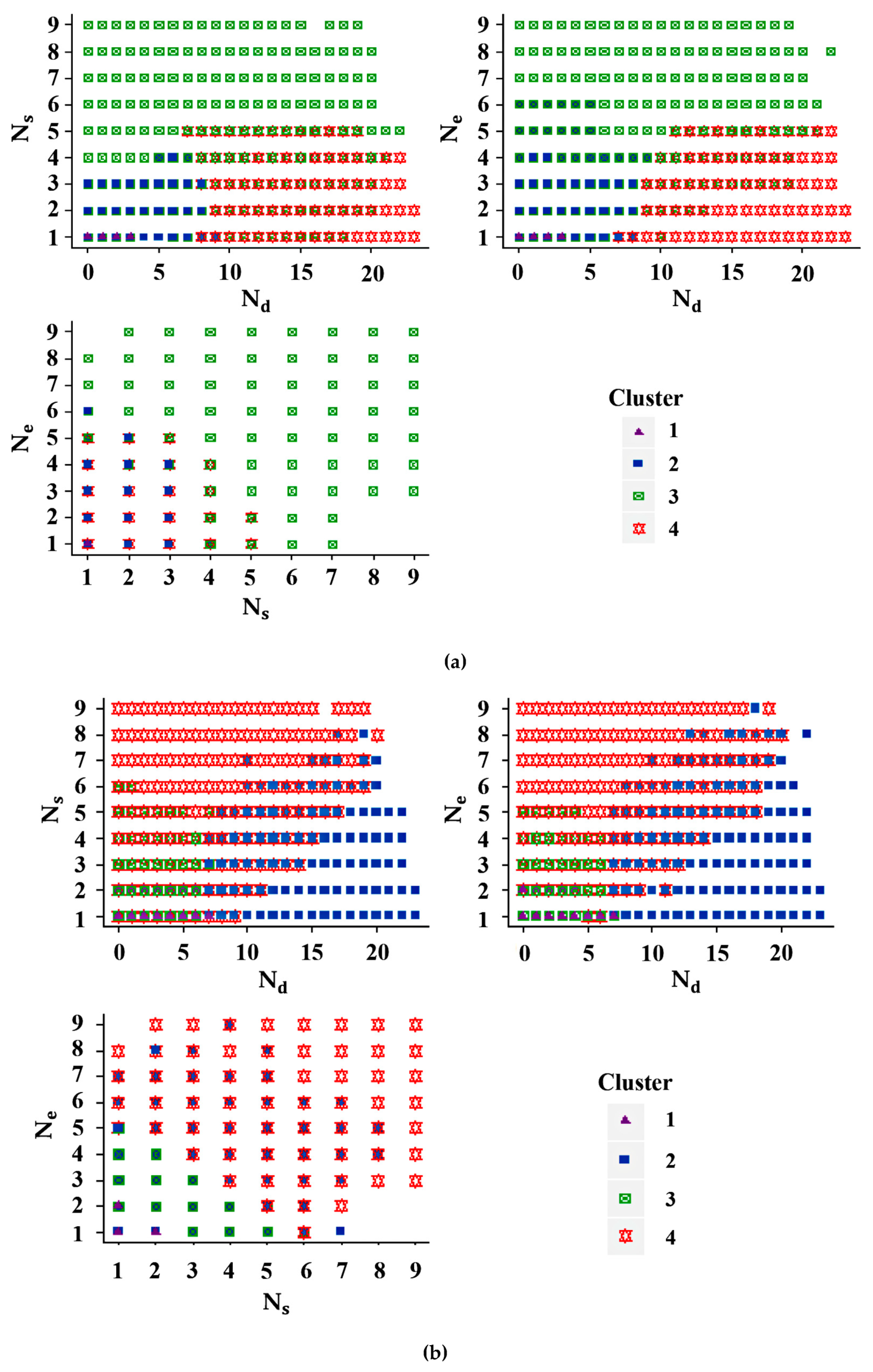
As shown in Figure 4, the commuters’ features were clustered into four clusters using Hclust and K-means, respectively. As introduced in Section 2.2, commuters tend to recur repeatedly (large ${\mathrm{N}}_{\mathrm{d}}$) during the fixed duration, a fixed origin (smaller ${\mathrm{N}}_{\mathrm{s}}$) and a fixed destination (smaller ${\mathrm{N}}_{\mathrm{e}}$) for multiple weekdays. Based on this, the Cluster 4 in Figure 4a and the Cluster 2 in Figure 4b were considered as the identified commuting vehicles and the other Clusters were labelled as non-commuting vehicles.

Figure 4. Clustering result with different methods. (a) Hclust method, (b) K-means method.

Specifically, it is believed that Cluster 1 and Cluster 2 in Figure 4a represented the travelers occasionally traveling through the test site at peak hours, and Cluster 3 in Figure 4a were the non-commuting travelers due to their flexible origins and destinations. Similar results can also be found in Figure 4b. A detailed description is shown in Table 3 for further analyzing the clustering results.

Table 3. Cluster centers, importance evaluation of features and performance evaluation for methods.

Method	Feature	Cluster					Performance Evaluation
		1	2	3	4	IMP	PF	$\overline{\mathbf{pf}}$	$\mathbf{V}$	$\mathit{l}/\mathbf{m}$
K-means	${\mathrm{N}}_{\mathrm{d}}$	0.2	12.3	0.9	2.8	0.11	3.34	2.64	0.05	0.07
	${\mathrm{N}}_{\mathrm{s}}$	1.0	2.1	2.2	4.0	0.10
	${\mathrm{N}}_{\mathrm{e}}$	1.1	2.7	2.4	4.6	0.10
Hclust	${\mathrm{N}}_{\mathrm{d}}$	0.1	1.1	3.9	13.6	0.10	3.47	2.79	0.04	0.05
	${\mathrm{N}}_{\mathrm{s}}$	1.0	2.1	4.1	2.0	0.09
	${\mathrm{N}}_{\mathrm{e}}$	1.0	2.3	4.6	2.5	0.11

Note: “Hclust” means “Ward’s hierarchical clustering” method, IMP means the quantification of the importance of a feature, PF is the performance evaluation indicator.

With labelled vehicles of commuters and non-commuters, an approach for performance evaluation was proposed between the proposed method and the traditional method. It was assumed that the better clustering method can identify more commuters with reasonable features (larger ${\mathrm{N}}_{\mathrm{d}}$ and ${\mathrm{N}}_{\mathrm{r}}$, smaller ${\mathrm{N}}_{\mathrm{s}}$ and ${\mathrm{N}}_{\mathrm{e}}$) and lower variance. To evaluate the methods, a performance evaluation indicator ($\mathrm{PF}$) was developed. The proposed evaluation metric $\mathrm{PF}$ reflects the reasonability of identified commuters’ features. A higher PF value indicates a more reasonable result of identified commuters. The proposed evaluation metric can improve the efficiency of determining the suitable method and increase the accuracy for commuters’ recognition. It is worth noting that as there are large differences in magnitude among the three features, ${\mathrm{N}}_{\mathrm{d}}^{\mathrm{i}},{\mathrm{N}}_{\mathrm{r}}^{\mathrm{i}},{\mathrm{N}}_{\mathrm{s}}^{\mathrm{i}}$ and ${\mathrm{N}}_{\mathrm{e}}^{\mathrm{i}}$ were rescaled as ${\mathrm{N}}_{\mathrm{d}}^{\mathrm{i}}{}^{\prime },{\mathrm{N}}_{\mathrm{r}}^{\mathrm{i}}{}^{\prime },{\mathrm{N}}_{\mathrm{s}}^{\mathrm{i}}{}^{\prime }$ and ${\mathrm{N}}_{\mathrm{e}}^{\mathrm{i}}{}^{\prime }$ to ensure the comparability of the variables. Take ${\mathrm{N}}_{\mathrm{d}}^{\mathrm{i}}$ as example, the detailed rescaling methods are expressed as Equation (15). The other formulas for performance evaluation are shown in Equations (16)–(18).

$${\mathrm{N}}_{\mathrm{d}}^{\mathrm{i}}{}^{\prime }=({\mathrm{N}}_{\mathrm{d}}^{\mathrm{i}}-\min ({\mathrm{N}}_{\mathrm{d}}^{\mathrm{i}}))/({\max (\mathrm{N}}_{\mathrm{d}}^{\mathrm{i}})-\min ({\mathrm{N}}_{\mathrm{d}}^{\mathrm{i}}))+1$$

(15)

$${\mathrm{pf}}_{\mathrm{i}}=({\mathrm{N}}_{\mathrm{d}}^{\mathrm{i}}{}^{\prime }+{\mathrm{N}}_{\mathrm{r}}^{\mathrm{i}}{}^{\prime })/{\mathrm{N}}_{\mathrm{s}}^{\mathrm{i}}{}^{\prime }+({\mathrm{N}}_{\mathrm{d}}^{\mathrm{i}}{}^{\prime }+{\mathrm{N}}_{\mathrm{r}}^{\mathrm{i}}{}^{\prime })/{\mathrm{N}}_{\mathrm{e}}^{\mathrm{i}}{}^{\prime }=({\mathrm{N}}_{\mathrm{d}}^{\mathrm{i}}{}^{\prime }+{\mathrm{N}}_{\mathrm{r}}^{\mathrm{i}}{}^{\prime })(\frac{{\mathrm{N}}_{\mathrm{s}}^{\mathrm{i}}{}^{\prime }+{\mathrm{N}}_{\mathrm{e}}^{\mathrm{i}}{}^{\prime }}{{\mathrm{N}}_{\mathrm{s}}^{\mathrm{i}}{}^{\prime }\ast {\mathrm{N}}_{\mathrm{e}}^{\mathrm{i}}{}^{\prime }})$$

(16)

$$\mathrm{V}=\mathrm{var}({\mathrm{N}}_{\mathrm{d}}^{\mathrm{i}}{}^{\prime })+\mathrm{var}({\mathrm{N}}_{\mathrm{r}}^{\mathrm{i}}{}^{\prime })+\mathrm{var}({\mathrm{N}}_{\mathrm{s}}^{\mathrm{i}}{}^{\prime })+\mathrm{var}({\mathrm{N}}_{\mathrm{e}}^{\mathrm{i}}{}^{\prime })$$

(17)

$$\mathrm{PF}=(l/\mathrm{m}\ast ({\displaystyle \sum }_{\mathrm{i}=1}^l{\mathrm{pf}}_{\mathrm{i}})/l)/\mathrm{V}$$

(18)

where ${\mathrm{pf}}_{\mathrm{i}}$ is the performance indicator for identified commuting vehicles, $\mathrm{m}$ and $\mathrm{l}$ are the total number of all vehicles and identified commuting vehicles, respectively, and $\mathrm{V}$ is the variance of features for identified commuting vehicles. The performance evaluation results are shown in Table 3. It was found that the identified commuters (displayed in gray background) had similar characters: larger ${\mathrm{N}}_{\mathrm{d}}$, smaller ${\mathrm{N}}_{\mathrm{s}}$ and smaller ${\mathrm{N}}_{\mathrm{e}}$, which indicates that both methods successfully identified the commuters. The importance of features was evaluated based on random forests [42]. Specifically, the importance ($\mathrm{IMP}$) of a feature was quantified by the impact of the feature’s permutation on the accuracy of the clustering results. For example, the importance of feature ${\mathrm{N}}_{\mathrm{d}}$ was derived by calculating the mean decrease accuracy of the clustering results through the model’s predicting after rearranging the order of values of ${\mathrm{N}}_{\mathrm{d}}$. The higher value of $\mathrm{IMP}$, the more significant it was to the clustering result. As expressed in Table 3, the values of $\mathrm{IMP}$ were similar, illustrating that the three features are of equal importance for the two methods.

For comparison, the performance evaluation indicators were derived using Equations (15)–(18). The higher $\mathrm{PF}$ value indicated that the method was more accurate in identifying commuters. As shown in Table 3, it was found that the Hclust method had a higher $\mathrm{PF}$ value. Specifically, the higher $l/\mathrm{m}$ value revealed that, compared with the Hclust method, more commuting vehicles were identified using the K-means method; lower $\mathrm{PF}$ illustrates a lower repeatability of temporal and spatial features using the K-means method; higher $\mathrm{V}$ means higher variance of commuting vehicles using the K-means method. The test site consisted of four lines: East line, West line, South line and North line. Given that commuters tend to have stable origins (on-ramps) or destinations (off-ramps), they were supposed to travel through the road network through two lines for work/home. Synthetically considering Figure 2 and Figure 4b, it was found that there were up to six destinations (off-ramps) for one line, however, the number of destinations for identified commuting vehicles varied from one to nine using the K-means method. That is to say, the identified commuters using the K-means method traveled through the road network through more than two lines. This is inconsistent with actual commuting behaviors. While for the Hclust method, all the three features of commuting vehicles were in accordance with that of the real world. Therefore, the Hclust method was utilized for commuting vehicles’ identification.

3.3. Commuting Pattern Analysis

To reveal the dynamic temporal-spatial features of commuting travels, the temporal and spatial commuting patterns were investigated based on the clustering results.

3.3.1. Temporal Commuting Pattern

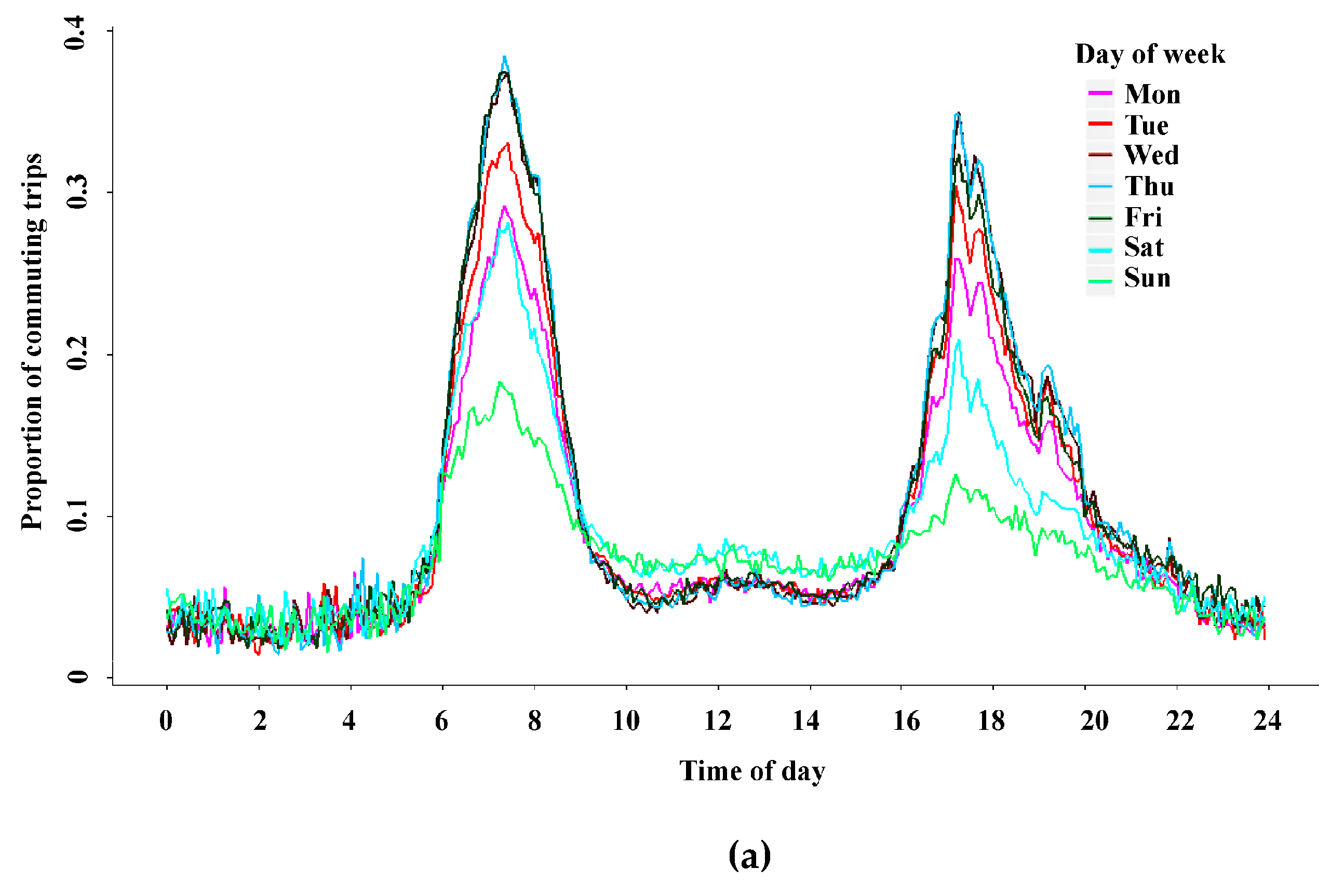
In terms of the temporal pattern, the time-of-day, day-of-week and day-to-day ratio of commuting trips of the test site was analyzed, respectively. The temporal commuting pattern was expressed as the average ratio of commuting trips at a specific duration. The ratio of commuting trips was considered as the proportion of commuting trips in the total number of trips at a period of time. For example, the time-of-day commuting pattern at different days of the week was derived as the average ratio of commuting trips at different days of the week.

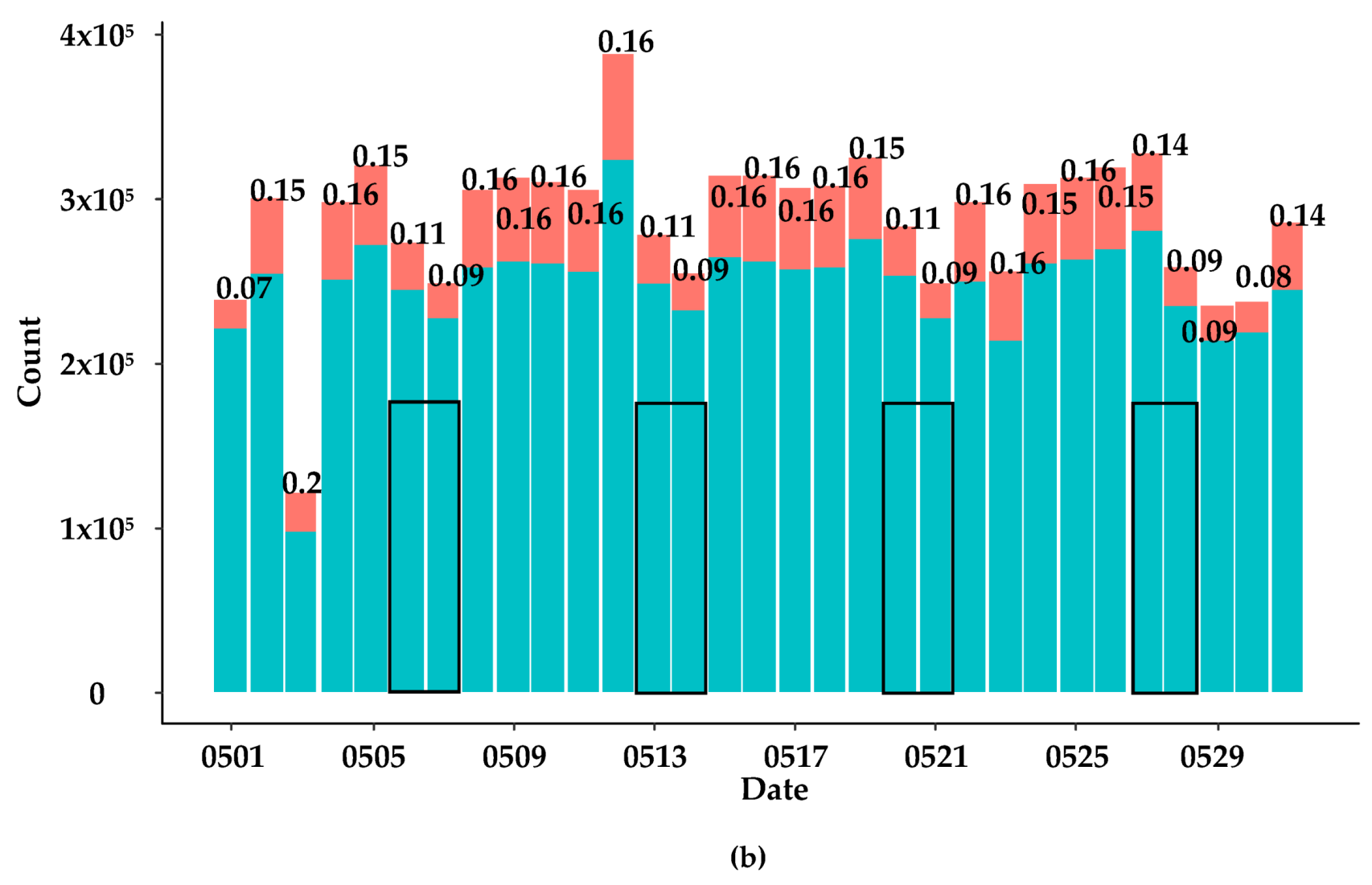
Figure 5a describes the average ratio of commuting trips every 5 min at different days of the week. It was shown that the overall ratio of commuting trips at morning peaks was larger and more concentrated compared to those at evening peaks. The reason is that the departure time at evening peaks is more flexible than that at morning peaks. Part of the commuters may go shopping or have dinner outside after work. Furthermore, the temporal commuting pattern was similar from Monday to Saturday, and the ratio of commuting trips at some peak hours of the weekdays reached 0.4. Besides, the daily traffic demands and their structure are shown in Figure 5b. The red and green rectangles describe the number of commuting and non-commuting trips, respectively. The labels are the ratios of commuting trips in a whole day. It shows that the ratio of commuting trips is relatively stable around 0.16 per day and the traffic demand is smaller on weekends (marked with black rectangles).

Figure 5. Temporal commuting pattern. (a) The ratio of commuting trips for time of day and day of week, (b) the daily number of commuting trips and total number of trips.

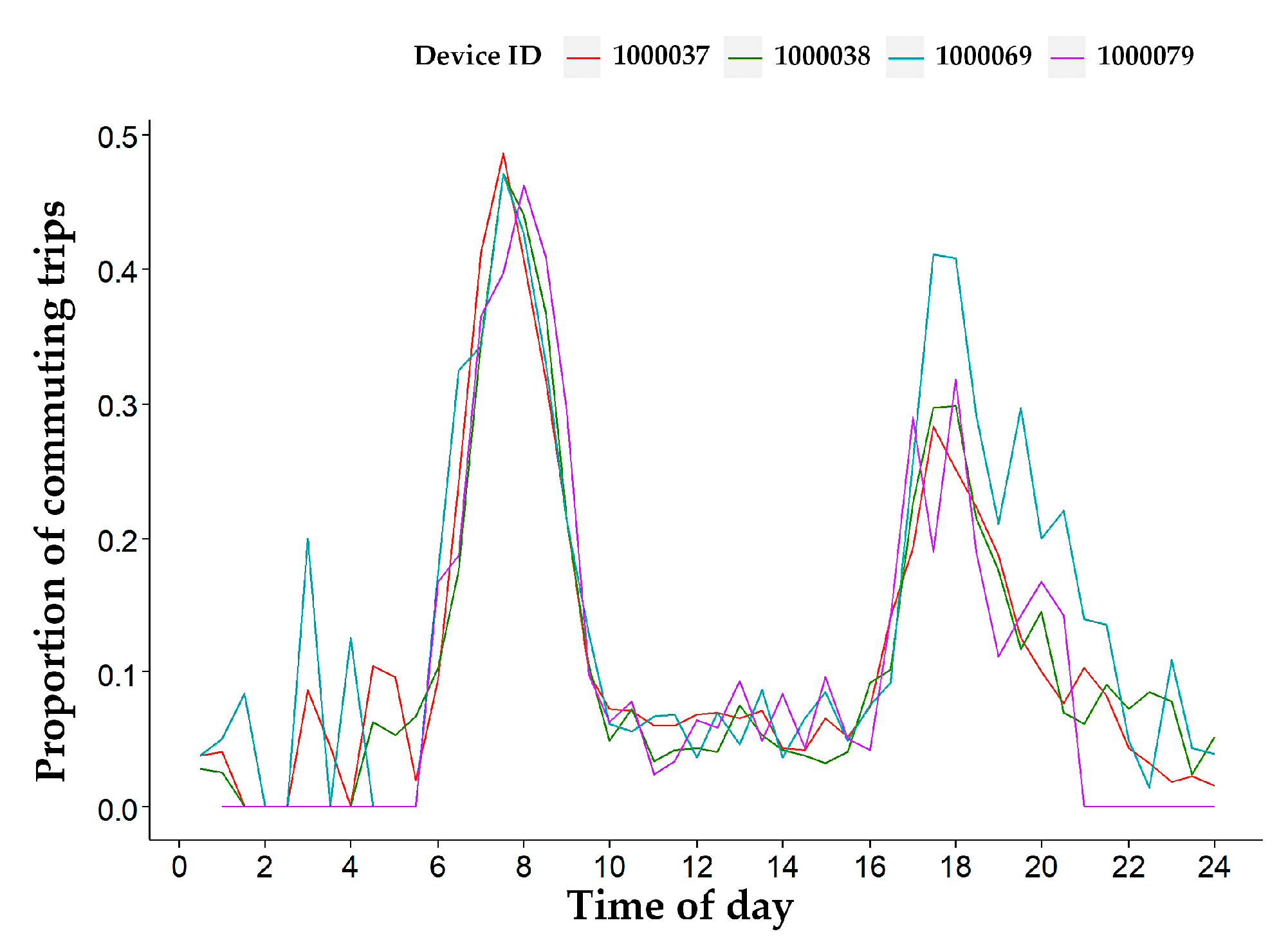
To characterize a more detailed temporal pattern, the ratio of commuting trips of partial frequently used ramps was analyzed. Figure 6 describes the ratios of commuting trips for device 1000037, 1000038, 1000069 and 1000079 on Tuesday, 16 May 2017. It shows that, compared with the average ratio of all ramps, these frequently used ones tend to have larger ratios of commuting trips, and the maximum ratio at some periods for these ramps is close to 0.5. These facilities are installed at ramps with higher ratios of commuting trips which have a greater impact on the selected network. It is necessary to meter or operate theses frequently used ramps to improve the efficiency of the network traffic.

Figure 6. The ratio of commuting trips of partial frequently used ramps on 16 May 2017.

3.3.2. Spatial Commuting Pattern

To investigate the spatial commuting pattern at the test site, the location-varying average ratio of commuting trips at AM/PM peak in different weekdays was analyzed. The AM and PM peak (7:00–9:00 and 17:00–19:00) was derived from the results in the previous section. Specifically, the spatial commuting pattern at AM (PM) peak was derived by averaging the ratios of commuting trips during 7:00–9:00 (17:00–19:00) at all the weekdays for each device.

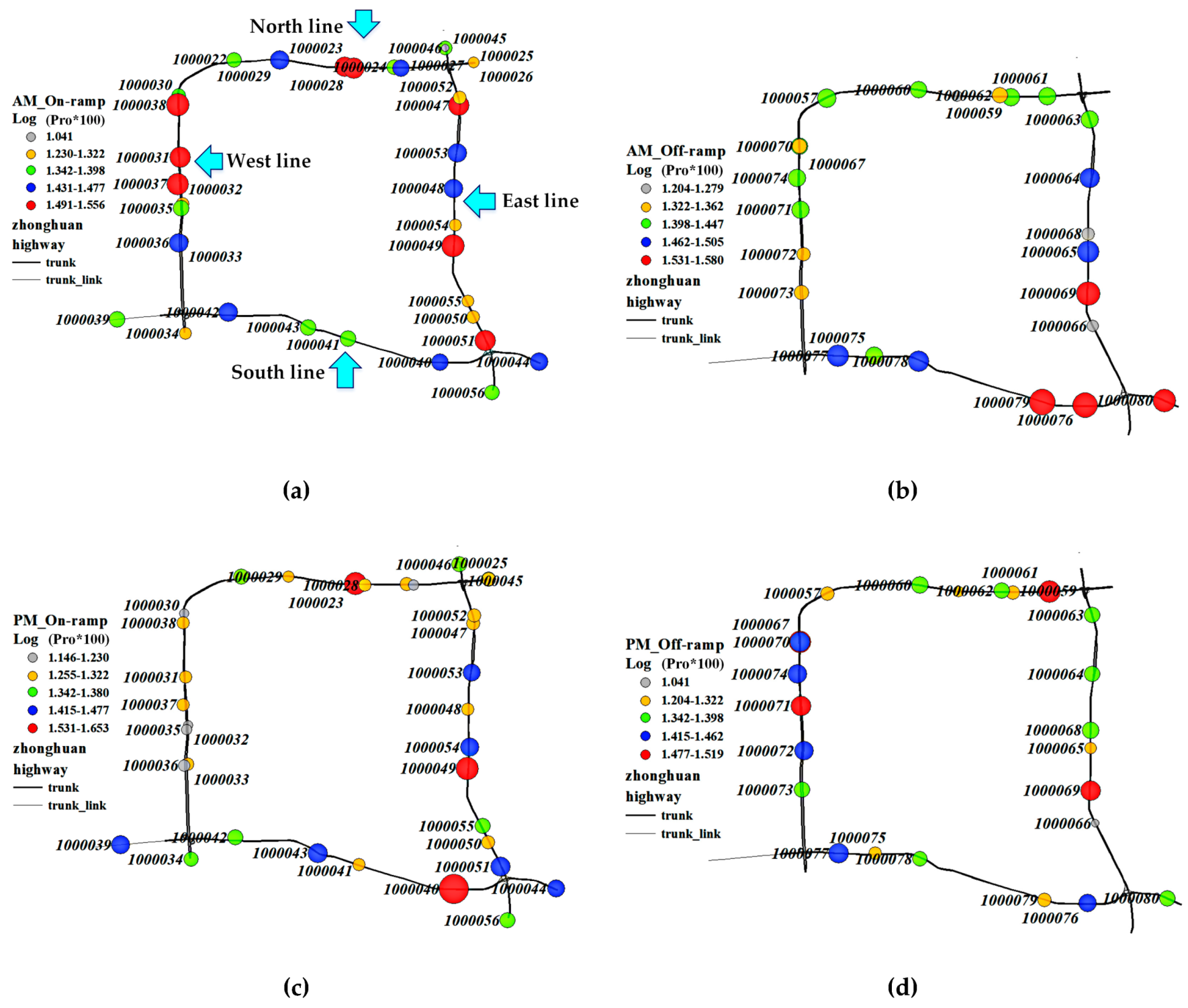
Figure 7a–d illustrates the spatial distribution of location-varying commuting pattern of ALPR devices at the AM and PM peak, respectively. It was observed that the spatial distributions of the ratio of commuting trips at the morning peak and evening peak have significant differences. Briefly, the test site was divided into four parts: East line, West line, South line, North line. For the AM peak, the origins (on-ramps) with a higher ratio of commuting trips were widely located in all these four lines while the destinations (off-ramps) with a higher ratio of commuting trips were distributed around the area where the East line and the South line meets together. Given the fact that Kunshan is a satellite city of the Shanghai metropolitan and this area is close to a widely used freeway to Shanghai, it implies that this area is frequently used by commuters who live in Kunshan and work in Shanghai. As for the PM peak, most of the origins with a higher ratio of commuting trips was also located in the East line and the South line. The consistency of the origins and destinations with a higher ratio of commuting trips for the PM and AM peaks implies the rationality of the commuters’ identification. Besides, it was observed that most of the destinations with a higher ratio of commuting trips during the evening peak were in the West line. Considering that the west of the test site in Kunshan city is a residential area, the result is in accordance with the traffic demands in the real world.

Figure 7. The commuting pattern of location-varying devices. (a) On-ramps at morning peak, (b) off-ramps at morning peak, (c) on-ramps at evening peak, (d) off-ramps at evening peak.

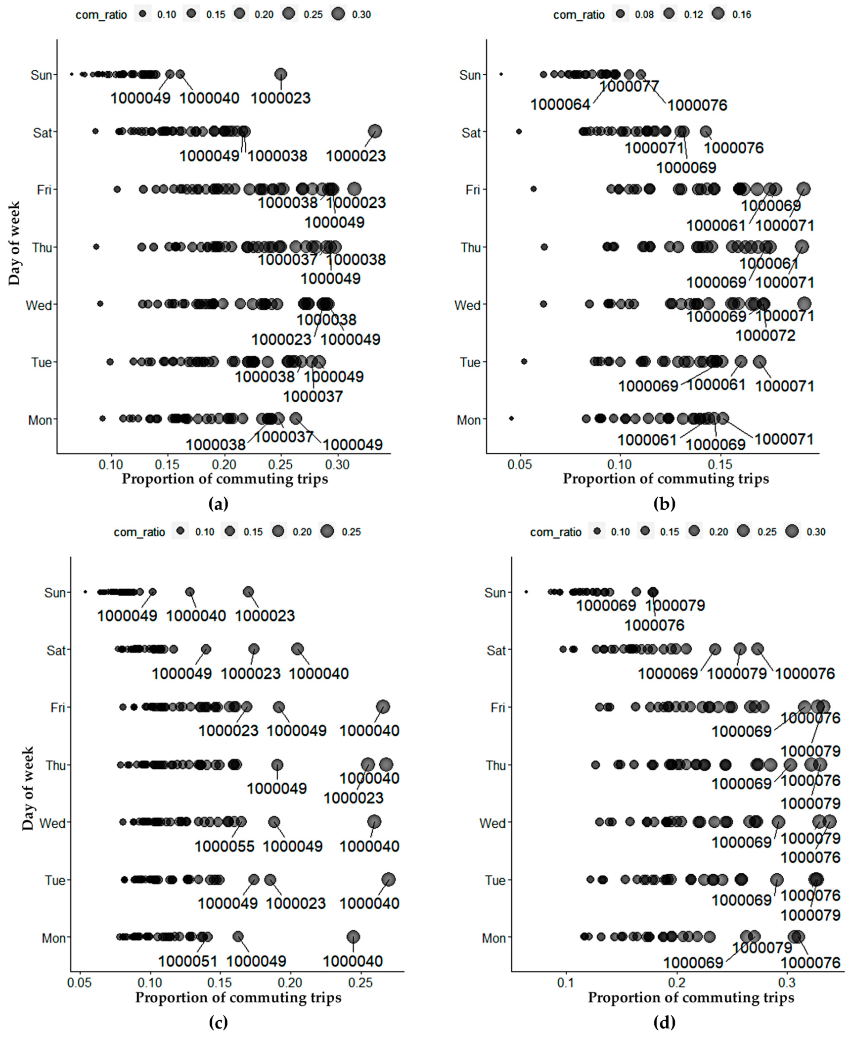
To further analyze the spatial commuting pattern, the location-varying ratio of commuting trips at days of the week were investigated in the morning and evening, respectively. The spatial commuting pattern in the morning and evening were derived by averaging the ratio of commuting trips before and after 12:00 on different days of the week for each device. Figure 8a,b depict the ratio of commuting trips of each device in the morning for on-ramps and in the evening for off-ramps. Similarly, Figure 8c,d depict the ratio of commuting trips for each device in the evening for the on-ramp and in the morning for the off-ramp, respectively. The ALPR devices installed at on-ramps were labelled from “1000022” to “1000056,” and the rest were installed at off-ramps. The large points with labelled numbers were the devices with the top three highest ratios of commuting trips at corresponding mornings/evenings on different days of week, which were considered to be frequently used ramps.

Figure 8. The pattern of location-varying ratio of commuting trips. (a) in the morning of on-ramp, (b) in the evening of off-ramp, (c) in the evening of on-ramp, (d) in the morning of off-ramp.

The comparison between frequently used ramps in Figure 8a,b and Figure 8c,d reveal that there were distinct correspondence relations between the frequently used on-ramps at AM and the frequently used off-ramps at PM, and the details of the correspondence relation are described as follows:

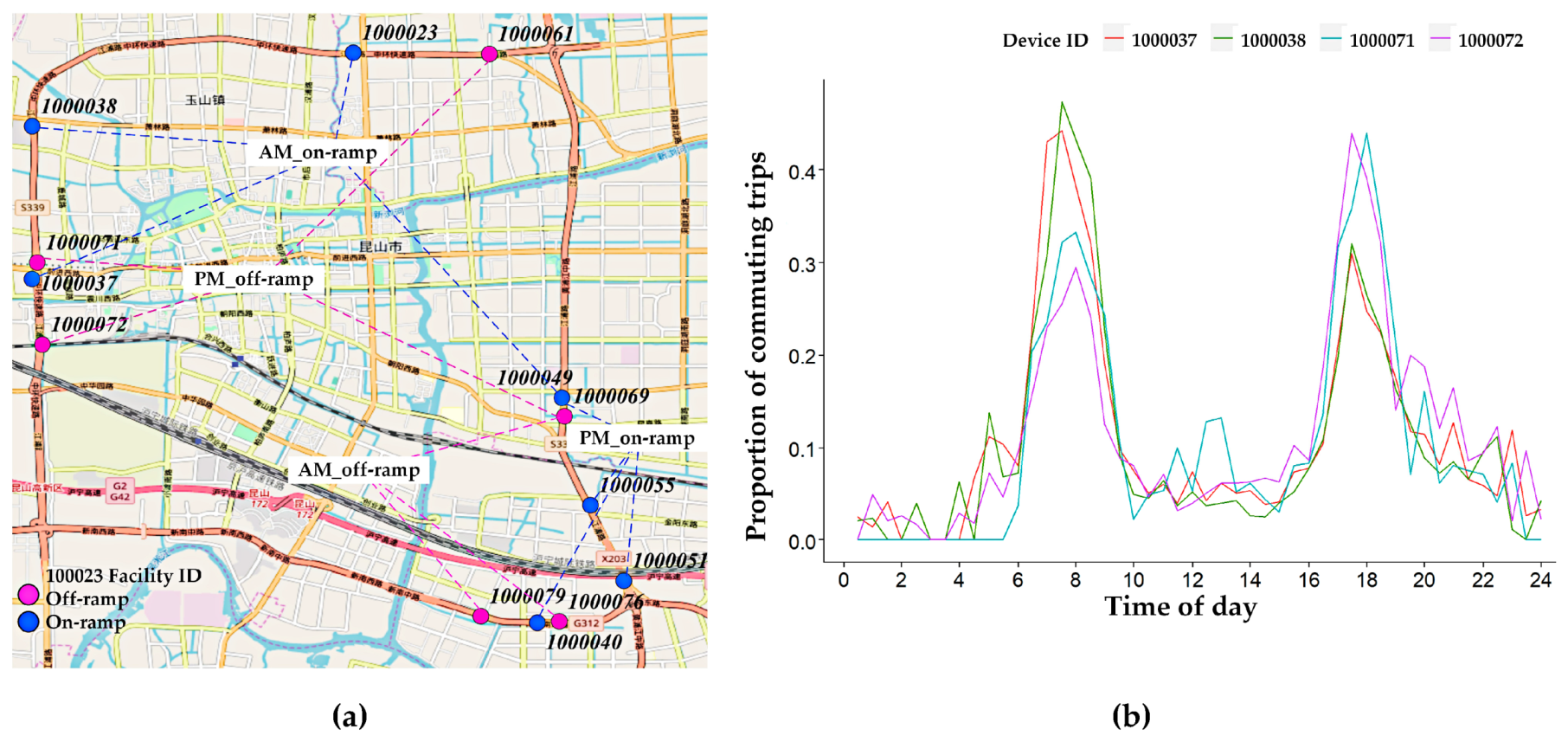
Figure 9a displays the locations of frequently used ramps at AM and PM in Figure 8. The on-ramps and off-ramps are distinguished with blue and red circles, respectively. The frequently used on-ramps and off-ramps at AM and PM are categorized by connected dotted lines. It was found that there were distinct correspondence relations between the frequently used on-ramps at AM and the frequently used off-ramps at PM. Take part of the frequently used ramps as an example, “1000023” was next to “1000061” in the North line, “1000049” was adjacent to “1000069” in the East line, “1000037,” “1000038” were next to “1000071,” “1000072” in the West line. Similar findings can also be found in Figure 8c,d, such as “1000049,” “1000051,” “1000055,” and “1000069” were close together in the East line, “1000040” was adjacent to “1000076,” “1000079” in the South line, etc. The results validated the consistency of commuting behaviors; it also illustrates that the proposed method is accurate.

Figure 9. The locations and time of day ratio of commuting trips for partial ramps. (a) The locations of frequently used ramps for AM and PM, (b) the ratio of commuting trips of partial frequently used ramps on 18 May 2017.

Finally, Figure 8d illustrates that the ratio of commuting trips of devices “1000076” and “1000079” were significantly higher in the morning than other devices. As shown in Figure 9a, the device “1000040” which was close to devices “1000076” and “1000079” also had a significantly higher ratio of commuting trips in the evening than other devices. Considering that all three devices were close to a widely used freeway, it implies that many people who live in Kunshan have jobs in Shanghai. Specifically, many home-to-work commuting trips from Kunshan to Shanghai were detected by the devices “1000076” and “1000079” on weekday mornings. Many work-to-home commuting trips from Shanghai to Kunshan were detected by the device “1000040”on weekday evenings.

Figure 9b describes the time of day ratio of commuting trips for device 1000037, 1000038, 1000071 and 1000072 on Thursday, 18 May 2017. Devices 1000037 and 1000038 were installed at on-ramps, and devices 1000071 and 1000072 were installed at off-ramps. The four frequently used ramps were close to each other (as shown in Figure 9a). Figure 9b indicates that the ratio of commuting trips of on-ramps in the AM was larger than 0.4 and the ratio of commuting trips of off-ramps in the PM was larger than 0.4. The opposite changing trend illustrates a correspondence relation between the origins and destinations for commuters. The consistent commuting behaviors illustrates the reasonability of the proposed method.

4. Conclusions

This paper developed a method which can accurately identify the commuters and proposed a systematic framework for commuting pattern recognition to support decision-making in practical applications. The characteristics of a commuting pattern for urban road networks were explored using ALPR data. The temporal and spatial features of individual vehicles were extracted and classified using Ward’s hierarchical clustering (Hclust) in order to identify the commuting vehicles. Comparison between the proposed method and traditional method (Hclust and K-means) was performed to evaluate the reasonability of the proposed clustering method and the indicator $\mathrm{PF}$ that characterized the commuters’ features was developed. The dendrogram and the $\mathrm{CHI}$ were utilized to determine the optimal number of clusters for the Hclust and K-means method. Based on this, a case study was conducted in Kunshan city, China. The comparison results demonstrated that the Hclust method performed better.

The proposed method investigated the temporal and spatial pattern of commuters. The findings in our paper can be summarized as follows: (1) the exploration of the temporal commuting pattern showed that the ratio of commuting trips for a whole day was relatively stable around 0.16 at weekdays, and the ratio of commuting trips at partial peaks of weekdays reached 0.4; (2) the exploration of the spatial commuting pattern revealed distinct correspondence relations between the frequently used on-ramps and off-ramps. The results validated the consistency of commuters’ behaviors, which can be a proof of the reasonability of the proposed method; (3) a pair of off-ramps in the morning and an on-ramps in the evening which were next to each other had significantly higher ratios of commuting trips. The reasons were analyzed with the properties of land use and demographic information of the test site. In the future, the impact of commuting patterns on the distribution of network traffic congestion will be investigated. More field validation works are needed to further interpret the commuting pattern.

References

- Hu, Y.; Wang, F. Temporal trends of intra urban commuting in Baton Rouge, 1990–2010. Ann. Am. Assoc. Geogr. 2016, 106, 470–479. [Google Scholar]
- McGuckin, N.; Fucci, A. Summary of Travel Trends: 2017 National Household Travel Survey, Report No: FHWA-PL-18-019; U.S. Department of Transportation, Federal Highway Administration: Washington, DC, USA, 2018.
- Varga, L.; Toth, G.; Neda, Z. Commuting patterns: The flow and jump model and supporting data. EPJ Data Sci. 2018, 7, 1–13. [Google Scholar] [CrossRef]
- Uboe, J. Aggregation of gravity models for journeys to work. Environ. Plan. A 2004, 36, 715–729. [Google Scholar] [CrossRef]
- Simini, F.; Gonzalez, M.C.; Maritan, A.; Barabasi, A.L. A universal model for mobility and migration patterns. Nature 2012, 484, 96–100. [Google Scholar] [CrossRef] [PubMed]
- Stefanouli, M.; Polyzos, S. Gravity vs radiation model: Two approaches on commuting in Greece. Transp. Res. Procedia 2017, 24, 65–72. [Google Scholar] [CrossRef]
- Masucci, A.P.; Serras, J.; Johansson, A.; Batty, M. Gravity versus radiation models: On the importance of scale and heterogeneity in commuting flows. Phys. Rev. E. 2013, 88. [Google Scholar] [CrossRef] [PubMed]
- Gargiulo, F.; Lenormand, M.; Huet, S.; Espinosa, O.B. Commuting network models: Getting the essentials. J. Artif. Soc. Soc. Simul. 2012, 15. [Google Scholar] [CrossRef]
- Tsiotas, D.; Aspridis, G.; Gavardinas, I.; Sdrolias, L.; Skodova-Parmova, D. Gravity modeling in social science: The case of the commuting phenomenon in Greece. Evol. Inst. Econ. Rev. 2019, 16, 139–158. [Google Scholar] [CrossRef]
- Bhat, C. Modeling the commute activity-travel pattern of workers: Formulation and empirical analysis. Transp. Sci. 2001, 35, 61–79. [Google Scholar] [CrossRef]
- Wan, L.; Gao, S.; Wu, C.; Jin, Y.; Mao, M.; Yang, L. Big data and urban system model-substitutes or complements? A case study of modelling commuting patterns in beijing. Comp. Environ. Urban Syst. 2018, 68, 64–77. [Google Scholar] [CrossRef]
- Polyzos, S.; Tsiotas, D.; Minetos, D. Determining the Driving Factors of Commuting: An Empirical Analysis from Greece. J. Eng. Sci. Technol. Rev. 2013, 6, 46–55. [Google Scholar] [CrossRef]
- Batty, M. Big data, smart cities and city planning. Dialogues Hum. Geogr. 2013, 3, 274–279. [Google Scholar] [CrossRef] [PubMed]
- Kahaki, S.M.M.; Nordin, M.J.; Ashtari, A.H. Incident and traffic-bottleneck detection algorithm in high-resolution remote sensing imagery. J. ICT Res. Appl. 2012, 6, 151–170. [Google Scholar] [CrossRef][Green Version]
- Kahaki, S.M.M.; Fathy, M.; Ganj, M. Road-following and traffic analysis using high-resolution remote sensing imagery. In Proceedings of the 3rd International Workshop on Intelligent Vehicle Controls and Intelligent Transportation Systems, Milan, Italy, 4–5 July 2009; pp. 133–142. [Google Scholar]
- Kahaki, S.M.M.; Nordin, M.D.J.; Ashtari, A.H. Incident detection algorithm based on radon transform using high-resolution remote sensing imagery. In Proceedings of the 2011 International Conference on Electrical Engineering and Informatics, Bandung, Indonesia, 17–19 July 2011. [Google Scholar]
- Zhou, D.; Hong, R.; Xia, J. Identification of taxi pick-up and drop-off hotspots using the density-based spatial clustering method. In Proceedings of the 17th COTA International Conference of Transportation Professionals, Shanghai, China, 7–8 July 2018. [Google Scholar]
- Kung, K.; Greco, K.; Sobolevsky, S.; Ratti, C. Exploring universal patterns in human home-work commuting from mobile phone data. PLoS ONE 2014, 9. [Google Scholar] [CrossRef] [PubMed]
- Altintasi, O.; Tuydesyaman, H. Utilization of RFID data to evaluate characteristics of private car commuters in Middle East Technical University campus. Pamukkale Univ. J. Eng. Sci. 2016, 22, 171–177. [Google Scholar] [CrossRef]
- Ma, X.; Liu, C.; Wen, H.; Wang, Y. Understanding commuting patterns using transit smart card data. J. Transp. Geogr. 2017, 58, 135–145. [Google Scholar] [CrossRef]
- McNeill, G.; Bright, J.; Hale, S.A. Estimating local commuting patterns from geolocated Twitter data. EPJ Data Sci. 2017, 6, 1–16. [Google Scholar] [CrossRef]
- Ortega-Tong, M. Classification of London’s Public Transport Users Using Smart Card Data. Ph.D. Thesis, Massachusetts Institute of Technology, Cambridge, MA, USA, 2013. [Google Scholar]
- Chang, Y.; Yang, D. Recognition of Vehicles with Commuting Property Using License Plate Data. J. Transp. Syst. Eng. Inf. Technol. 2016, 16, 77–82. (In Chinese) [Google Scholar]
- Chen, H.; Yang, C.; Xu, X. Clustering vehicle temporal and spatial travel behavior using license plate recognition data. J. Adv. Transp. 2017, 2017. [Google Scholar] [CrossRef]
- Rao, W.; Wu, Y.J.; Xia, J.; Ou, J.; Kluger, R. Origin-destination pattern estimation based on trajectory reconstruction using automatic license plate recognition data. Transp. Res. Part C Emerg. Technol. 2018, 95, 29–46. [Google Scholar] [CrossRef]
- Ou, J.; Lu, J.; Xia, J.; An, C.; Lu, Z. Learn, Assign, and Search: Real-Time Estimation of Dynamic Origin-Destination Flows Using Machine Learning Algorithms. IEEE Access 2019, 7, 26967–26983. [Google Scholar] [CrossRef]
- Ou, J.; Xia, J.; Wu, Y.-J.; Rao, W. Short-term traffic flow forecasting for urban roads using data-driven feature selection strategy and Bias-corrected random forests. Transp. Res. Rec. 2019, 2645, 157–167. [Google Scholar] [CrossRef]
- Ozturk, F.; Ozen, F. A new license plate recognition system based on probabilistic neural networks. Procedia Technol. 2012, 1, 124–128. [Google Scholar] [CrossRef]
- Primerano, F.; Taylor, M.A.P.; Pitaksringkarn, L.; Tisato, P. Defining and understanding trip chaining behaviour. Transportation 2008, 35, 55–72. [Google Scholar] [CrossRef]
- Kim, J.; Mahmassani, H.S. Spatial and temporal characterization of travel patterns in a traffic network using vehicle trajectories. Transp. Res. Procedia 2015, 9, 164–184. [Google Scholar] [CrossRef]
- Rao, W.; Xia, J.; Lyu, W.; Lu, Z. Interval data-based k-means clustering method for traffic state identification at urban intersections. IET Intell. Transp. Syst. 2019, 13, 1106–1115. [Google Scholar] [CrossRef]
- Oh, S.; Byon, Y.-J.; Yeo, H. Impact of Traffic State Transition and Oscillation on Highway Performance with Section-Based Approach. In Proceedings of the Intelligent Transportation Systems (ITSC) 2015, IEEE 18th International Conference on IEEE, Las Palmas, Spain, 15–18 September 2015; pp. 2141–2146. [Google Scholar]
- Fraley, C.; Raftery, A.E. Model-based clustering, discriminant analysis, and density estimation. J. Am. Stat. Assoc. 2002, 97, 611–631. [Google Scholar] [CrossRef]
- Xia, J.; Chen, M. A nested clustering technique for freeway operating condition classification. Comput.-Aided Civ. Infrastruct. Eng. 2007, 22, 430–437. [Google Scholar] [CrossRef]
- Xia, J.; Huang, W.; Guo, J. A clustering approach to online freeway traffic state identification using ITS data. KSCE J. Civil Eng. 2012, 16, 426–432. [Google Scholar] [CrossRef]
- Murtagh, F.; Legendre, P. Ward’s Hierarchical Clustering Method: Clustering Criterion and Agglomerative Algorithm. Available online: https://arxiv.org/pdf/1111.6285.pdf (accessed on 25 December 2019).
- Ou, J.; Xia, J.; Wang, Y.; Wang, C.; Lu, Z. A data-driven approach to determining freeway incident impact areas with fuzzy and graph theory-based clustering. Comput.-Aided Civ. Infrastruct. Eng. 2020, 35, 178–199. [Google Scholar] [CrossRef]
- Ou, J.; Yang, S.; Wu, Y.-J.; An, C.; Xia, J. Systematic clustering method to identify and characterise spatiotemporal congestion on freeway corridors. IET Intell. Transp. Syst. 2018, 12, 826–837. [Google Scholar] [CrossRef]
- Dragut, A.; Nichitiu, C. A monotonic on-line linear algorithm for hierarchical agglomerative classification. Inf. Technol. Manag. 2004, 5, 114–141. [Google Scholar] [CrossRef]
- Rani, Y.; Rohil, H. A study of hierarchical clustering algorithm. Int. J. Inf. Comput. Technol. 2013, 3, 1225–1232. [Google Scholar]
- Liu, Y.; Li, Z.; Xiong, H.; Gao, X.; Wu, J. Understanding of Internal Clustering Validation Measures. In Proceedings of the 2010 IEEE International Conference on Data Mining, Sydney, Australia, 14–17 December 2010. [Google Scholar]
- Strobl, C.; Boulesteix, A.L.; Kneib, T.; Augustin, T.; Zeileis, A. Conditional variable importance for random forests. BMC Bioinform. 2008, 9. [Google Scholar] [CrossRef]
© 2020 by the authors. Licensee MDPI, Basel, Switzerland. This article is an open access article distributed under the terms and conditions of the Creative Commons Attribution (CC BY) license (http://creativecommons.org/licenses/by/4.0/).