Abstract
The pattern of urban land use and the level of urbanization in China’s pre-modernization period are of great significance for land use and land cover change (LUCC) research. The purpose of this study is to construct a 1910s spatial dataset of provincial land urbanization in pre-modern China. Using historical topographic maps, this study quantitatively reconstructs the built-up area of various cities in Zhejiang Province in the 1910s. The research indicates that: (1) During the early period of the Republic of China, there were a total of 252 cities and towns in Zhejiang Province, including 75 cities at or above the county level, 21 acropolis, and 156 towns. The total built-up area was 140.590 km2. (2) The county-level urbanization level had significant agglomeration characteristics. The overall urbanization rate of land was 0.135%. (3) Hot spots analysis showed that the Hang-Jia-Hu-Shao plain is hot spot. (4) The correlation coefficient between the city wall perimeter data recorded in the local chronicles and the measured city wall perimeter was 0.908. The research showed that the military topographic maps possessed a good application prospect for the reconstruction of urbanization levels. The research results provide direct evidence for urbanization and urban land use in China’s pre-modernization period.
1. Introduction
Land use and land cover change (LUCC) is one of the primary ways human activities affect the earth system [1], and it has complex regional and global ecological environmental impacts and responses. Among the various land cover changes, urbanized areas are the most severe form. Urbanization is the process of transforming agriculturally oriented areas into non-agricultural forms by changing the land use structures [2,3]. Unreasonable urbanization may cause serious ecological and environmental problems [4], such as the reduction of forests [5] and arable land [6], and the destruction of the rivers network [7] and wetlands [8]. These are all issues that must be faced in sustainable development; long-term sequences of urban land use processes can provide basic data for this research [9].
The urbanization process is an important indicator that reflects regional development. In the past 100 years, global urbanization has developed rapidly. The world urbanization level rose from 16.4% in 1900 to 46.8% in 2000 [10]. According to United Nations forecasts, 68% of the world population will live in urban areas by 2050 [11,12]. Since World War II, with the economic development, the level of urbanization in many developing countries has increased significantly. The urbanization level in India increased from 17% in 1950 to 32% in 2015 and in Brazil it increased from 47% in 1950 to 82% in 2015 [13]. Among the major industrialized large countries, the urbanization level in Russia increased from 44% in 1950 to 74% in 2015 and in the United States it increased from 74% in 1950 to 81% in 2015 [14]. With the rapid development of China’s society and economy after the reform and opening, China’s urbanization level also increased from 18% in 1978 to nearly 60% in 2018 [15,16]. Many scholars have begun to explore the historical background of this phenomenon from the viewpoint of the evolution of Chinese urban development [17]. Relevant studies [18,19] have shown that, in addition to military and political factors, the development of cities and towns during the historical period was closely related to the development of commercial industries. In particular, the rise of commercial towns in the Jiangnan region, which primarily includes Jiangsu and Zhejiang Provinces, since the period of the Republic of China (1911–1949), has played an important role in pre-industrial urbanization [19,20]. Due to missing related statistics, some scholars have estimated the level of urbanization during Chinese historical periods. For example, G. William Skinner [21,22] estimated that the level of urbanization in the Jiangnan region was approximately 10% at the end of the 19th century. Chen [23] used survey data from the government of the Republic of China to study the level of urbanization of the population in Jiangnan. The results showed that the level of urbanization during the 1930s was approximately 15%. Since most of these studies are speculative analyses, further quantitative analyses are yet to be conducted.
In addition, some scholars have begun to try to reconstruct the spatial patterns of urban and rural construction land during the middle of the Qing Dynasty (1644–1911) based on an allocation model under the control of statistical materials [19]. Some analyses showed that [24,25], based on the allocation model, only the potential land use pattern could be obtained, not the actual land cover. Therefore, more direct data are needed for the reconstruction of historical urban land spatial patterns. Remote sensing image data are generally only approximately 40 years old [26,27]. Hence, other types of data sources are urgently needed to reconstruct the urbanization level and spatial patterns of the past 100 years and during pre-modern China.
Historical military topographic maps and old maps play a very important role in land use reconstruction [28], urbanization development [29], and ecological assessment [30,31]. Combined with GIS and remote sensing information [32], historical topographic maps can provide different kind of historical land use change information for decades to over 200 years [28,33,34], such as the geomorphological evolution of the plain [35], archaeological survey [36], landscape and land use changes [37,38,39], and hydrological environment [29,40]. In recent years, with the exploitation of a series of historical military topographic map data, topographic maps that were completed in the early 20th century are employed to be crucial data sources for historical urban land use reconstruction in China [41,42,43]. Studies have shown that [44,45] military topographic maps during the period of the Republic of China were completed based on modern surveying and mapping techniques, and their errors were generally between 1/4000 and 1/1000. In addition, because urban areas have important military value, this type of topographic map has a more detailed mapping of towns and surrounding areas [46]. During this period, the military topographic maps marked urban areas in accordance with the unified standard [47] (Figure 1). In particular, urban areas were drawn with city walls or color blocks, which can be identified easily and used for urban land reconstruction. In this study, the urbanized areas above the town level in Zhejiang Province (Figure 2), which belongs to a core area of Jiangnan, is utilized as the research object. Then, according to the military topographic map data produced during the Republic of China, an exploratory spatial data analysis (ESDA) in the ArcGIS platform is used to perform a spatial analysis and area calculation. The research results can provide historically basic data for the study of urbanization in pre-modern China. In addition, the urbanization data series can be extended by approximately a century.
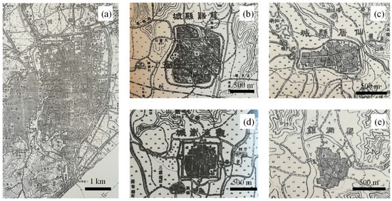
Figure 1.
Systematic illustration of the Zhejiang military topographic maps (1:50,000) in the Republic of China. (a) Hangxian County (1913); (b) Cixi County (1916); (c) Xianju County (1920); (d) Guanhai Acropolis (1916); and (e) Liangtong Town (1916).
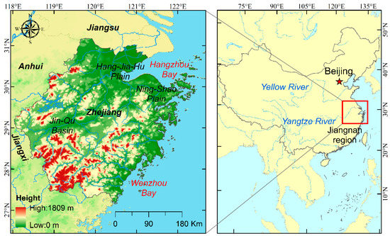
Figure 2.
Location and topographic maps of Zhejiang Province.
2. Study Area, Materials, and Methods
2.1. Study Area
The study area of this article is Zhejiang Province (27°02′–31°11′ N, 118°01′–123°10′ E), which is located in the southeast coastal area of China. The total area is 105,500 km2 and the terrain is sloping from southwest to northeast, with various landform types. Zhejiang Province is located in the middle of the subtropical zone and belongs to a monsoon humid climate with superior natural conditions [48]. The civilization of this area has been developed since ancient times and belongs to the traditional developed area in China [49].
In general, cities are large settlements formed by the aggregation of non-agricultural industries and non-agricultural population, including both small towns and large cities [50]. According to the Chinese traditional city classification criteria [18], it can be divided into a provincial capital city, prefecture-level cities, county-level cities, and other towns. Zhejiang Province is divided into 12 prefectures (Figure 3), and each prefecture is divided into several counties. The political center of Zhejiang Province is Hangzhou Fu, which belongs to the prefecture level, and the provincial capital city is Hangxian county. Other prefectures include Jiaxing, Huzhou, Jinhua, Quzhou, Yanzhou, Ningbo, Shaoxing, Wenzhou, Taizhou, Chuzhou, and Dinghai. There are 75 county-level administrative units, and the scope of jurisdiction is basically the same as that of modern Zhejiang Province. The boundaries of the administrative units at the prefecture and county levels were drawn based on the CHGIS-1911 dataset jointly developed by Fudan University and Harvard University [51]. Except for cities above the county level, the remaining urbanized areas are mainly towns, which provided commercial services to rural areas. It is worth noting that there is a special type of acropolis in the town of Zhejiang Province. This type of acropolis was originally a military castle, and gradually developed into a commercial town [52].
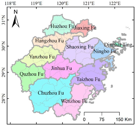
Figure 3.
Administrative division map of Zhejiang Province in 1911.
2.2. Military Topographic Map
The historical maps used in this study were primarily the military topographic maps of Zhejiang Province during the period of the Republic of China archived in the Key Laboratory of the Poyang Lake Wetland and Watershed Research Ministry of Education, Jiangxi Normal University. This set of topographic maps primarily consists of large-scale maps of 1:50,000. The mapping time was from the Republic of China year two (AD 1913) to the Republic of China year 25 (AD 1936), covering the entire province of Zhejiang and including parts of the Jiangxi, Anhui, and Jiangsu Provinces. The surveying and mapping organization was the Zhejiang Army Survey Bureau during the early stage. It was later changed to the Zhejiang Land Survey Bureau of the Staff Headquarters of the National Government. There are 345 maps of the whole province, and the size of each picture is approximately 46 cm × 35 cm. The longitude span of each map is 15′, and the latitude span is 10′. The elevation system assumes that the altitude of the Ziwei Garden in the old provincial Administration of Zhejiang is 50 m. The map schema adopts the original topographic map of the Republic of China year three (AD 1914). For a small portion of the missing area, topographic maps collected by the former National Government’s Ministry of the Interior organized by the Institute of the Modern History Academia Sinica were used as a supplement [53].
Another source of military topographic maps used in this study was a 1950s aerial survey map from the U.S. Army with a scale of 1:250,000. During the Anti-Japanese War, the Sino-US Cooperative Aerial Survey Team [54] conducted detailed aerial photogrammetry of eastern China. In the early 1950s, the Army Map Service of the US Corps of Engineers produced a set of 1:250,000 topographic maps of eastern China based on aerial survey data [55]. These are now archived in the University of Texas Library Pavilion [56]. This set of maps has detailed latitude and longitude information and projection properties that were used for spatial correction and information extraction during the early stage. Compared with this set of 1:50,000 military topographic maps of the Republic of China, aerial survey maps have better spatial coordinate information, so they can use the same place name points for spatial referencing and improve accuracy. Although the scales of the two sets of topographic maps are different, we extract all map information in the ArcGIS 10.2 platform based on the results of geographic referencing, and guarantee the reliability of the results through fine-tuning and compared with remote sensing imagery.
2.3. Spatiotemporal Scope
Since this study only involved the urban areas and towns in this set of topographic maps, the period statistics of the maps without relevant town information in the map were not counted. The mapping time of the related maps was primarily concentrated between 1913 and 1936 (Figure 4a), with a median of 1917 (Figure 4b). Among them, the highest frequency occurred in 1916, accounting for approximately 25%. Therefore, it can be considered that this set of military topographic maps basically reflects the urban and town construction information of Zhejiang Province during the early period of the Republic of China. The scope of this study is Zhejiang Province during the early period of the Republic of China.
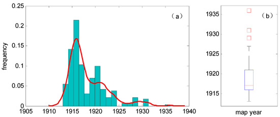
Figure 4.
Histogram (a) and box plot (b) of the period of this set of military topographic maps.
2.4. Process Flow and the GIS-ESDA Model
The research process of this study primarily included the following three steps (Figure 5). First, based on the detailed spatial coordinate information of the 1950s aerial survey map from the U.S. Army, a preliminary georeferencing of the set of 1:50,000 military topographic maps from the 1910s was performed. Then the position of the preliminary located topographic map was fine-tuned based on the remote sensing image to ensure the accuracy of the spatial information. Finally, based on the Zipf rule and the GIS-ESDA model, a spatial analysis and area measurement of the urban information on the historical topographic map was completed.
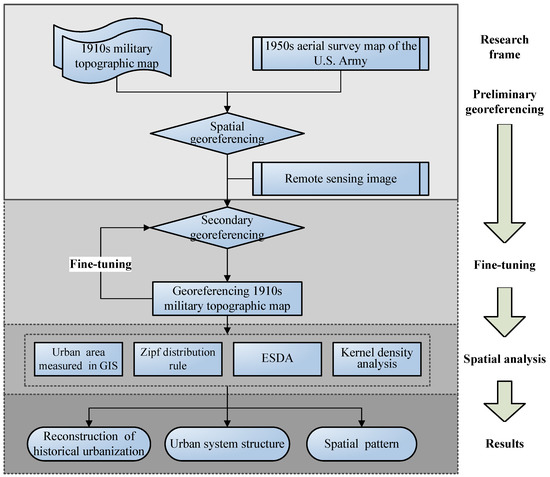
Figure 5.
Process flow and the GIS-ESDA model.
2.4.1. Preliminary Georeferencing
The spatial positioning of this set of topographic maps primarily included two steps. First, this set of topographic maps were initially registered and positioned in the ArcGIS 10.2 platform according to the stitching relationship. Second, based on the space coordinate information of the aerial map from the US military, the military map of the 1910s was spatially located according to some same place names and mountains or rivers.
2.4.2. Fine-Tuning of Topographic Map
Fine-tuning of topographic map primarily included two steps. First, modern Landsat satellite TM/ETM+ remote sensing images [57] were used to repeatedly fine-tune the position of the topographic map based on obvious natural landmarks (such as mountains and rivers). Second, control points were utilized for overall error control and evaluation.
2.4.3. Spatial Analysis
Zipf Distribution Rule
It is generally believed that the size distribution of cities in the different levels in a region follows a certain law. G. K. Zipf proposed the law in 1949:
where Si is the scale of the i-th city; S0 is the scale of the first city; and Ri is the rank of the i-th city. In view of the fact that the Zipf distribution law is an ideal state of order-scale distribution in cities, it is generally expressed in terms of the Rotka model [58,59]:
where q is the fractal dimension of the urban system. Generally, the logarithm of both sides of Equation (2) can be taken to obtain:
Then the fractal dimension, q, is obtained using the method of least squares. Studies [60] have shown that when q > 1, the distribution of urban systems in the region is more concentrated, and large cities are prominent. When q < 1, the distribution of urban systems in the region is relatively scattered, and small or medium cities develop.
Exploratory Spatial Data Analysis, the ESDA
The ESDA is a collection of spatial data analysis technologies. It primarily reveals spatial correlation characteristics and patterns by studying the spatial heterogeneity of data and the visualization of spatial distribution patterns [61]. The ESDA mainly includes a global spatial autocorrelation, a local spatial autocorrelation, a hotspot analysis, and a spatial trend analysis.
This study used the Moran’s I index for the global spatial autocorrelation analysis [62,63]. The larger the Moran’s I index, the higher the degree of spatial autocorrelation in the region. The calculation method is:
where n is the number of sample points; yi and yj are the attribute values of the sample points; and wij is the spatial weight matrix.
The local spatial autocorrelation was identified using the Getis-Ord Gi* index [62,63]. The Gi* index is normalized, and the Z value is obtained. A higher Z value indicates that this area is a hot spot gathering area, while a lower Z value indicates that this area is a cold spot gathering area. The calculation method for the Z value of the Getis-Ord Gi* index is:
where n is the number of sample points; xi and yj are the attribute values of the sample points; and wij is the spatial weight matrix.
Kernel Density Analysis
Kernel density analysis is a non-parametric test method that can be used to analyze the density of spatial point distributions. The basic principle is to estimate the theoretical distribution of sample points in a region using a kernel density function and to convert the density of discrete sample points into density values that are continuously distributed in space. A kernel density analysis can identify the concentrated area of a spatial point feature distribution; that is, the hotspot distribution area. The calculation method is:
where k (·) is the kernel function; r is the analysis radius; and x − xi is the distance between the point x to be estimated and the sample point xi.
GeoDa and ArcGIS Platforms
The calculation process involved in this study was mainly performed using GeoDa 0.9.5 and ArcGIS 10.2 software platforms. The main calculation indicators include the Moran’s I Index, the Getis-Ord Gi* index, and the kernel density value.
3. Results
3.1. Reconstruction of Urban Built up Areas
Based on the measured topographic maps of the urban areas, the spatial distribution (Figure 6a) and built-up area (Figure 6b) of each city or town were obtained using the ArcGIS 10.2 platform. Statistics show that during the period of the Republic of China (Table 1), there were a total of 252 cities and towns of various types in the Zhejiang Province, including 75 cities at the county level and above, 21 acropolises, and 156 towns. The total built-up area of towns and cities in the province was 140.590 km2, of which the total built-up area of cities at the county level and above was 91.764 km2, with an average value of 1.223 km2. The total built-up area of acropolises was 8.051 km2, with an average value of 0.383 km2. The total built-up area of towns was 40.775 km2, with an average value of 0.261 km2. Of all of the cities and towns in Zhejiang Province, the largest built-up area was Hangxian, which is the capital city of the province, with an area of 14.778 km2. The smallest was Maqiao town, Haining County, with an area of only 0.023 km2.
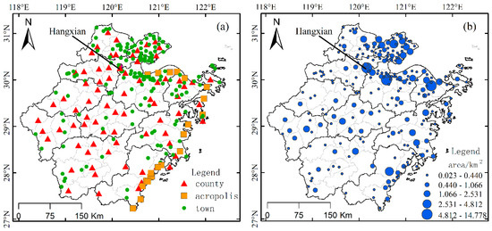
Figure 6.
Urban spatial distribution (a) and built-up area (b) of Zhejiang Province during the Republic of China.

Table 1.
Statistics of cities and towns in the Zhejiang Province.
3.2. Spatial Pattern of Urbanization
The level of urbanization can be measured from the perspectives of urbanization of land and urbanization of population. Because urban population data for historical periods are difficult to obtain, this study used the ratio of the total area of urban built-up areas and land area at the county level scale as urbanization rate.
With the support of GeoDa 0.9.5 and ArcGIS 10.2, the Moran’s I index Equation (7) of the county-level urbanization in Zhejiang Province during the 1910s was 0.296 (Z-Score = 4.992, p < 0.001). This indicated that its spatial distribution had significant agglomeration characteristics (Figure 7). More precisely, the high-value area of the urbanization level was adjacent to the high-value area, and the low-value area was adjacent to the low-value area.
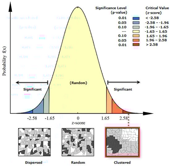
Figure 7.
Spatial autocorrelation characteristics of the urbanization level of Zhejiang Province in the Republic of China.
As can be seen from Figure 8a, among all county-level units, Hangxian County had the highest urbanization rate at 1.463%. Jingning County had the lowest at 0.014%, and the overall urbanization rate of Zhejiang Province was 0.135%. Further analysis of the local spatial autocorrelation cold and hot spots (Figure 8b) showed that the Z-score of the Getis-Ord Gi* index Equation (5) had obvious high–high/low–low aggregation characteristics in the spatial distribution. More precisely, the hot spots were primarily distributed in the Hang-Jia-Hu-Shao plain area nearby Hangzhou Bay, and the cold spot concentration areas were near west Zhejiang and southwest Zhejiang. The area near Wenzhou Bay belonged to the medium distribution area of the Z-score value. The spatial distribution of the cold and hot spots were generally in the direction of northeast–southwest; that is northeast Zhejiang Province belonged to hotspots and the southwest belonged to cold spots.
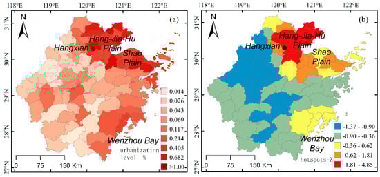
Figure 8.
Urbanization level at the county level (a) and the spatial hotspot distribution (b) of Zhejiang Province in the Republic of China.
3.3. Urban System Structure
The expressions of the rank-scale distribution of all of the 252 cities and towns in Zhejiang Province during the Republic of China were obtained using the Zipf distribution rule (Equations (1)–(3)): y = −1.010x + 3.352 (r2 = 0.903, p < 0.001). According to Equation (3), we can see that the fractal dimension is q = 1.010 >1. It can be seen that, as a whole, the distribution of the Zhejiang urban system was relatively concentrated during the 1910s. Furthermore, the kernel density analysis method Equation (6) in ArcGIS 10.2 was used to obtain the spatial pattern of all cities and towns in Zhejiang Province, such as cities at the county level and above, towns, and acropolises. From Figure 9a, it can be seen that the kernel density values of spatial distribution of all of the 252 cities and towns in Zhejiang Province during 1910s formed two high-value central areas on the north and south sides of Hangzhou Bay. In addition, two secondary nuclear density regions existed near the Ning-shao Plain and Wenzhou Bay. From Figure 9b, it can be clearly seen that the spatial distribution of 75 county-level cities and above in Zhejiang Province is evenly distributed, and no relatively high-value areas had been formed throughout the province. Since cities at the county level and above were basically political institutions in pre-modern China, their even spatial distribution is conducive to administrative control.
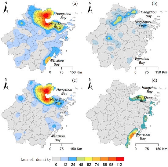
Figure 9.
Spatial distribution of the kernel density map of all the cities (a) county-level and above cities; (b) towns; (c) and acropolises (d).
Nevertheless, the spatial density of the county-level cities and above in northern Zhejiang was still higher than that in southern Zhejiang, which is consistent with the fact that the northern counties in Zhejiang are more distributed than the southern ones. According to the spatial distribution kernel density maps of 156 towns in the province (Figure 9c), it can be seen that the spatial distribution pattern is basically consistent with the spatial structure of all cities and towns in Zhejiang Province (Figure 9a). Moreover, a high value range of kernel density is primarily distributed on the both sides of Hangzhou Bay and areas such as the Ning-Shao Plain. This also shows that the urban system pattern of Zhejiang Province during the Republic of China was primarily determined by the spatial distribution of towns. The areas, such as the Hang-Jia-Hu Plain and the Ning-Shao Plain, have always developed market economies, so a large number of towns have developed under county-level cities. Due to historical reasons, such as resistance to pirating and coastal defenses, Zhejiang’s coastal areas also have had a large number of acropolises. From Figure 9d, it can be seen that the areas with high kernel density values in the urban spatial distribution of the acropolis are primarily concentrated along the coast of eastern Zhejiang and the southern shore of Hangzhou Bay. In addition, another high kernel density area formed in the Wenzhou Bay area.
3.4. Trend Analysis
From an analysis of the spatial trend of the built-up areas of all of the 252 cities and towns (Figure 10a), it can be seen that the distribution trend rises from west to east and rises from south to north. This also shows that the spatial distribution of all the urban areas in Zhejiang Province has a trend of being high in the northeast and low in the southwest. The spatial trend analysis of the urbanization level of the 75 county-level regions in Zhejiang Province also indicates this result (Figure 10b).
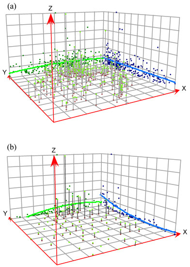
Figure 10.
Trend analysis of the built-up areas of cities and towns (a) and the urbanization level in Zhejiang Province (b). (x-axis arrow direction indicates east; y-axis arrow direction indicates north; z-axis arrow direction indicates built-up areas or the urbanization level.).
4. Discussion
4.1. Uncertainty Analysis
Although the military topographic map of the Republic of China used in the reconstruction of urban built-up areas in this study was completed using modern surveying and mapping technology, the technological conditions and cartographic levels at that time had historical limitations. Therefore, it is necessary to evaluate the errors of these topographic maps and perform an uncertainty analysis. By referring to the principle of the “point-to-point” test [26,42], 26 relevant control points were randomly selected in the military topographic map after secondary correction and fine-tuning according to the principle of uniform distribution throughout the province. These were then compared with the corresponding position in the TM/ETM+ remote sensing image. The error range between the control points on the remote sensing image and the points on the topographic map were calculated in ArcGIS 10.2 (Table 2), and error range distribution map was interpolated by kriging method in ArcGIS 10.2 (Figure 11). The error range of the 26 control points was between 0.142 and 1.348 km, and the average error was 0.553 km. Considering that these sets of military topographic maps had relatively small errors after secondary correction and projection fine-tuning, they can be used for the reconstruction of relevant geographical elements in this area.
Table 2.
Military topographic maps error range of Zhejiang Province in the Republic of China.
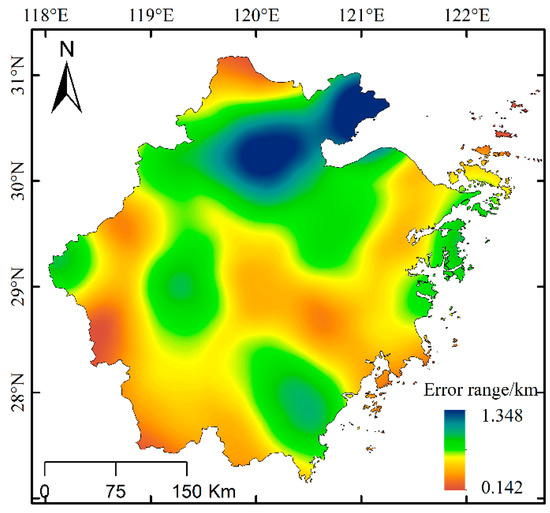
Figure 11.
Map of error range distribution in Zhejiang Province.
4.2. Comparison of the Perimeter of the City Wall and Historical Records
During the historical period, various national archives and chronicles have generally been recorded in the shape of the city and the perimeter of the city wall, but they are often described non-quantitatively in the form of text or hand-drawn maps. For example, during the Qing Dynasty (AD 1644–1911) in the Emperor Jiaqing Restoration Unification Book, the city wall form of Fuyang County in Zhejiang Province was recorded as “The perimeter is six li. Four gate. There is a ring moat around the city. Southeast of the city near the river …” He et al. [64] made full use of the city wall perimeter data recorded in the historical books and obtained the city area by considering the shape of the city as a square or a circle. They also obtained a set of built-up areas of cities in the 18 provinces of the Qing Dynasty. Since the construction of the city wall was basically not done in Zhejiang Province after the period of the Republic of China, the city information reflected on the topographic map of the Republic of China can be considered to represent the perimeter. Therefore, it can be considered the actual city wall shape and area of the city during the Qing Dynasty.
Based on the city wall perimeter data recorded in the local chronicles and in the Emperor Jiaqing Restoration Unification Book, the city wall perimeter information of 55 cities above the county level was obtained, including 12 prefecture-level cities. In addition, the unit of measurement of the length of the Qing Dynasty li was converted according to 1 li = 0.576 km [65], and the area formula is:
where Ai is the area of the i-th city; and Ci is the circumference of the i-th city. The city wall perimeter was converted into the area (km2). By comparing the historical city wall perimeter data and city wall perimeter data based on the topographic map of the Republic of China (Figure 12a), it was found that the correlation coefficient between the two groups reached 0.908 (p < 0.001). It can be seen that, although the city perimeter data recorded in the historical books are limited in terms of the approximate number and low precision, the overall length is significantly consistent with the actual city perimeter length reconstructed from the military topographic map. The results of the regression analysis showed that the city perimeter data recorded in the historical books was approximately 20% higher than the measured value. It should be noted that, since Hangxian is the capital of Zhejiang Province, it has a large wall perimeter and area than other cities. After excluding Hangxian data from the model, the correlation coefficient is 0.834 (p < 0.001).
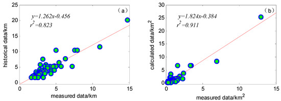
Figure 12.
Correlation of the city wall perimeter (a) or urban area (b) between historical data and measured data.
Similarly, there is a significant correlation between the measured city area and the city area calculated using Equation (7) (Figure 12b), and the correlation coefficient is 0.955 (p < 0.001). The area calculated using Equation (7) is approximately 80% higher than the measured area. The correlation coefficient is 0.843 (p < 0.001) after excluding Hangxian data from the model.
4.3. Comparison of Land Urbanization and Population Urbanization
Land urbanization and population urbanization are two aspects of the urbanization process. As detailed statistics of urban land and population in history are often subject to many limitations, the relationship between the two groups needs to be further examined. Fortunately, the Ministry of the Interior of the National Government during the period of the Republic of China conducted preliminary statistics on the population of counties in Zhejiang Province. The report “Statistics of Provinces, Cities, and Villages of Zhejiang Province” in the fourth Internal Affairs Survey Statistics Form in December 1933 published in detail the total population of counties and towns, with the exception of the provincial capital population. The records reported data from January 1931 to May 1933. This batch of data can be considered to reflect the population distribution of Zhejiang Province in the early and middle period of the Republic of China. In addition, the population data of Hangxian, the provincial capital, was supplemented by the Monthly Statistics (No. 26) of the Republic of China in 1934.
A regression analysis of the urban area of the county and the total population of the county in Zhejiang Province for the middle period of the Republic of China showed that the correlation coefficient between them was 0.792 (p < 0.001) (Figure 13a). It can be seen that there was a significant correlation between the urban area of the county and the total population. Generally, the area of the county with a large population has a larger urban built-up area. After excluding Hangxian data from the model, the correlation coefficient is 0.810 (p < 0.001). The reason for this change may be that Hangxian is the capital city of Zhejiang Province and has a high proportion of the urban population in the total population.
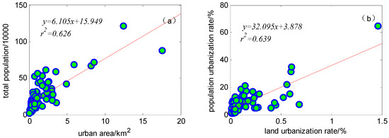
Figure 13.
(a) The relationship between the urban area and the total population of the county; (b) The relationship between land urbanization and population urbanization.
Although there was no direct urban demographic data in the Internal Affairs Survey Statistics Form, the county town population and general town population can be used to approximate the urban population in a certain county. In addition, the population urbanization level of the county can be obtained using this method. The calculation results showed that the overall population urbanization rate in Zhejiang Province was 13.49%, with the highest value of Hangxian being 64.71% and the lowest value of Qingyuan being 1.08%. The regression analysis of the land urbanization level and the population urbanization level showed that the correlation coefficient between them was 0.799 (p < 0.001) (Figure 13b). It should be noted that the reason for the high urbanization rate of the population in Hangxian County might be because the original data included the entire population of the provincial capital, but it did not distinguish between urban and agricultural populations. After excluding Hangxian data from the model, the correlation coefficient is 0.609 (p < 0.001). Despite this fact, the coupling relationship between land urbanization and population urbanization can still be studied using the two sets of data.
5. Conclusions and Prospects
(1) During the period of the Republic of China, there were a total of 252 cities and towns in Zhejiang Province including 75 cities at or above the county level, 21 cities in acropolis, and 156 towns. The total built-up area of towns and cities in the province was 140.590 km2, of which the total built-up area of cities at the county level and above was 91.764 km2, with an average value of 1.223 km2. The total built-up area of the acropolis was 8.051 km2, with an average value of 0.383 km2. In addition, the total built-up area of towns was 40.775 km2, with an average value of 0.261 km2.
(2) During the period of the Republic of China, the county-level urbanization level of Zhejiang Province had significant agglomeration characteristics. Among the county-level units, the urbanization rate was highest in Hangxian County at 1.463%, and lowest in Jingning County at 0.014%. The province’s overall land urbanization rate was 0.135%. An analysis of the cold and hot spots showed that the hot spots were primarily distributed in the Hang-Jia-Hu-Shao area near Hangzhou Bay. The cold spots were primarily concentrated in the western and southwestern Zhejiang. The region near Wenzhou Bay belonged to the medium distribution area of the Z value.
(3) According to the Zipf distribution rule, it was concluded that the distribution of Zhejiang’s urban system during the Republic of China belonged to the centralized distribution type. The results of the kernel density analysis showed that the urban spatial distribution formed two high-value central areas on the north and south sides of Hangzhou Bay and two secondary high-density areas near the Ning-Shao Plain and Wenzhou Bay.
(4) The correlation coefficient between the city wall perimeter data recorded in the local chronicles and the measured city wall perimeter was 0.908, showing that the historical books and chronicles had high reliability. However, the results of the regression analysis showed that the city perimeter data recorded in the historical books was approximately 20% higher than the measured value.
(5) The province’s overall urbanization rate was 13.49%, of which the highest value of Hangxian County was 64.71% and the lowest value of Qingyuan County was 1.08%. During the period of the Republic of China, there was a significant correlation between the urbanization rate of county land and the urbanization rate of the population, and the correlation coefficient was 0.799.
This study systematically demonstrated the relationship between the city wall perimeter data in historical local chronicles and the measured urban built-up area using the 1:50,000 large-scale topographic map data during the Republic of China, which was in pre-modern China. Additionally, according to the regression analysis, the relational equation of the historical city wall perimeter and the measured urban area was obtained. Most parts of China have relatively systematic historical records of the city wall perimeter that can be converted to the urban area using the relationship formula, thus providing basic data for a long-term urbanization level sequence study. In addition, by performing a comparison with the population data of Zhejiang Province during the Republic of China, the correlation between the land urbanization and the population urbanization data was obtained. This correlation provides an empirical research result for understanding the relationship between different measures of urbanization during historical periods.
However, due to the accuracy limitations of historical data, the urban built-up area reconstructed in this paper can only represent the situation in the early and middle period of the Republic of China. The coupling relationship between land urbanization and population urbanization is only a preliminary discussion. Later land-use reconstruction work requires in-depth research on the spatial projection correction and the control of reconstruction errors to ensure the reliability of reconstruction data. Additionally, the spatial and temporal resolution of land use reconstruction for an historical period should be further improved, and the dynamic pattern evolution analysis of land use and urbanization should be performed on a more detailed scale.
Author Contributions
Z.W. and F.L. conceived and designed the experiments; Z.W., X.C., M.J. (Min Ju), C.L. and M.J. (Meixin Jiang) performed the model; Z.W., G.L. and Y.J. analyzed the data; Z.W. wrote the paper. All authors have read and agreed to the published version of the manuscript.
Funding
This research was funded by National Natural Science Foundation of China (41761045 and 41561020) and Open fund of Shandong Provincial Key Laboratory of Water and Soil Conservation and Environmental Protection (STKF201909).
Acknowledgments
We thank anonymous referees and the editor for their helpful comments on this paper. We thank LetPub (www.letpub.com) for its linguistic assistance during the preparation of this manuscript.
Conflicts of Interest
The authors declare no conflict of interest.
References
- Brovkin, V.; Ganopolski, A.; Claussen, M.; Kubatzki, C.; Petoukhov, V. Modelling climate response to historical land cover change: GCTE/LUCC research letter. Glob. Ecol. Biogeogr. 1999, 8, 509–517. [Google Scholar] [CrossRef]
- Gödecke, T.; Waibel, H. Rural-urban transformation and village economy in emerging market economies during economic crisis: Empirical evidence from Thailand. Camb. J. Reg. Econ. Soc. 2011, 4, 205–219. [Google Scholar] [CrossRef]
- Antrop, M. Landscape change and the urbanization process in Europe. Landsc. Urban Plan 2004, 67, 9–26. [Google Scholar] [CrossRef]
- Chen, M.; Liu, W.; Lu, D. Challenges and the way forward in China’s new-type urbanization. Land Use Policy 2016, 55, 334–339. [Google Scholar] [CrossRef]
- Delphin, S.; Escobedo, F.J.; Abd-Elrahman, A.; Cropper, W.P. Urbanization as a land use change driver of forest ecosystem services. Land Use Policy 2016, 54, 188–199. [Google Scholar] [CrossRef]
- García-Nieto, A.P.; Geijzendorffer, I.R.; Baró, F.; Roche, P.K.; Bondeau, A.; Cramer, W. Impacts of urbanization around Mediterranean cities: Changes in ecosystem service supply. Ecol. Indic. 2018, 91, 589–606. [Google Scholar] [CrossRef]
- Yousefi, S.; Moradi, H.R.; Keesstra, S.; Pourghasemi, H.R.; Navratil, O.; Hooke, J. Effects of urbanization on river morphology of the Talar River, Mazandarn Province, Iran. Geocarto Int. 2019, 34, 276–292. [Google Scholar] [CrossRef]
- Matchett, E.L.; Fleskes, J.P. Projected impacts of climate, urbanization, water management, and wetland restoration on waterbird habitat in California’s Central Valley. PLoS ONE 2017, 12, e169780. [Google Scholar] [CrossRef] [PubMed]
- Xu, H.; Zhang, W. The causal relationship between carbon emissions and land urbanization quality: A panel data analysis for Chinese provinces. J. Clean. Prod. 2016, 137, 241–248. [Google Scholar] [CrossRef]
- Klein Goldewijk, K.; Beusen, A.; Janssen, P. Long-term dynamic modeling of global population and built-up area in a spatially explicit way: HYDE 3.1. Holocene 2010, 20, 565–573. [Google Scholar] [CrossRef]
- Bloom, D.E. 7 billion and counting. Science 2011, 333, 562–569. [Google Scholar] [CrossRef] [PubMed]
- United Nations Department of Affairs. 68% of the World Population Projected to Live in Urban Areas by 2050. Available online: https://www.un.org/development/desa/en/news.html (accessed on 4 January 2020).
- Chauvin, J.P.; Glaeser, E.; Ma, Y.; Tobio, K. What is different about urbanization in rich and poor countries? Cities in Brazil, China, India and the United States. J. Urban Econ. 2017, 98, 17–49. [Google Scholar] [CrossRef]
- Department of Economic and United Nations. World Urbanization Prospects: The 2018 Revision. Available online: https://population.un.org/wup/Download/ (accessed on 4 January 2020).
- Wang, X.; Hui, E.C.; Choguill, C.; Jia, S. The new urbanization policy in China: Which way forward? Habitat Int. 2015, 47, 279–284. [Google Scholar] [CrossRef]
- Wu, H.; Hao, Y.; Weng, J. How does energy consumption affect China’s urbanization? New evidence from dynamic threshold panel models. Energy Policy 2019, 127, 24–38. [Google Scholar] [CrossRef]
- Jiang, W. The urban form of traditional mid-small cities: Focus on cadastral maps of Jurong county town in the Republic China. J. Chin. Hist. Geogr. 2014, 29, 33–45. [Google Scholar]
- Gu, C.; Chai, Y.; Cai, J. Chinese Urban Geography; The Commercial Press: Beijing, China, 1999; pp. 1–703. [Google Scholar]
- Xie, J.; Jin, X.; Lin, Y.; Cheng, Y.; Yang, X.; Bai, Q.; Zhou, Y. Quantitative estimation and spatial reconstruction of urban and rural construction land in Jiangsu Province, 1820–1985. J. Geogr. Sci. 2017, 27, 1185–1208. [Google Scholar] [CrossRef]
- Jin, X.; Cao, X.; Du, X.; Yang, X.; Bai, Q.; Zhou, Y. Farmland dataset reconstruction and farmland change analysis in China during 1661-1985. J. Geogr. Sci. 2015, 25, 1058–1074. [Google Scholar] [CrossRef]
- Skinner, G.W.; Baker, H.D. The City in Late Imperial China; Stanford University Press: Redwood City, CA, USA, 1977. [Google Scholar]
- Skinner, G.W. Rural marketing in China: Repression and revival. China Q. 1985, 103, 393–413. [Google Scholar] [CrossRef]
- Chen, X. Changes in Population and Urbanization Level of Jiangnan Towns in Modern Times. Zhejiang Acad. J. 1996, 34, 113–117. [Google Scholar]
- Yang, X.; Guo, B.; Jin, X.; Long, Y.; Zhou, Y. Reconstructing spatial distribution of historical cropland in China’s traditional cultivated region: Methods and case study. Chin. Geogr. Sci. 2015, 25, 629–643. [Google Scholar] [CrossRef]
- Yang, X.; Jin, X.; Lin, Y.; Han, J.; Zhou, Y. Review on China’s spatially-explicit historical land cover datasets and reconstruction methods. Prog. Geogr. 2016, 35, 159–172. [Google Scholar] [CrossRef]
- Wan, Z.; Jia, Y.; Hong, Y.; Liu, G.; Jiang, M. Evolution of Jingjiang Section of the Yangtze River Based on Historical Maps and Remote Sensing over the Past 100 Years. Sci. Geogr. Sin. 2019, 39, 696–704. [Google Scholar] [CrossRef]
- Li, S.; Bing, Z.; Jin, G. Spatially explicit mapping of soil conservation service in monetary units due to land use/cover change for the Three Gorges Reservoir Area, China. Remote Sens. 2019, 11, 468. [Google Scholar] [CrossRef]
- Statuto, D.; Cillis, G.; Picuno, P. Using historical maps within a GIS to analyze two centuries of rural landscape changes in Southern Italy. Land 2017, 6, 65. [Google Scholar] [CrossRef]
- Bae, S.; Chang, H. Urbanization and floods in the Seoul Metropolitan area of South Korea: What old maps tell us. Int. J. Disaster Risk Reduct 2019. [Google Scholar] [CrossRef]
- Nicu, I.C. Tracking natural and anthropic risks from historical maps as a tool for cultural heritage assessment: A case study. Environ. Earth Sci. 2017, 76, 1–15. [Google Scholar] [CrossRef]
- Jedlička, J.; Havlíček, M.; Dostál, I.; Huzlík, J.; Skokanová, H. Assessing relationships between land use changes and the development of a road network in the Hodonín region (Czech Republic). Quaest. Geogr. 2019, 38, 145–159. [Google Scholar] [CrossRef]
- Agapiou, A.; Lysandrou, V.; Alexakis, D.D.; Themistocleous, K.; Cuca, B.; Argyriou, A.; Sarris, A.; Hadjimitsis, D.G. Cultural heritage management and monitoring using remote sensing data and GIS: The case study of Paphos area, Cyprus. Comput. Environ. Urban Syst. 2015, 54, 230–239. [Google Scholar] [CrossRef]
- Pindozzi, S.; Cervelli, E.; Capolupo, A.; Okello, C.; Boccia, L. Using historical maps to analyze two hundred years of land cover changes: Case study of Sorrento peninsula (south Italy). Cartogr. Geogr. Inf. Sci. 2016, 43, 250–265. [Google Scholar] [CrossRef]
- Dhanani, A. Suburban built form and street network development in London, 1880–2013: An application of quantitative historical methods. Hist. Methods 2016, 49, 230–243. [Google Scholar] [CrossRef]
- Furlanetto, P.; Bondesan, A. Geomorphological evolution of the plain between the Livenza and Piave Rivers in the sixteenth and seventeenth centuries inferred by historical maps analysis (Mainland of Venice, Northeastern Italy). J. Maps 2015, 11, 261–266. [Google Scholar] [CrossRef][Green Version]
- Rondelli, B.; Stride, S.; García-Granero, J.J. Soviet military maps and archaeological survey in the Samarkand region. J. Cult. Herit. 2013, 14, 270–276. [Google Scholar] [CrossRef]
- San-Antonio-Gómez, C.; Velilla, C.; Manzano-Agugliaro, F. Urban and landscape changes through historical maps: The Real Sitio of Aranjuez (1775–2005), a case study. Comput. Environ. Urban Syst. 2014, 44, 47–58. [Google Scholar] [CrossRef]
- Schaffer, G.; Levin, N. Reconstructing nineteenth century landscapes from historical maps-the Survey of Western Palestine as a case study. Landsc. Res. 2016, 41, 360–379. [Google Scholar] [CrossRef]
- Nicu, I.C.; Stoleriu, C.C. Land use changes and dynamics over the last century around churches of Moldavia, Bukovina, Northern Romania-Challenges and future perspectives. Habitat Int. 2019, 88, 101979. [Google Scholar] [CrossRef]
- Pavelková, R.; Frajer, J.; Havlíček, M.; Netopil, P.; Rozkošný, M.; David, V.; Dzuráková, M.; Šarapatka, B. Historical ponds of the Czech Republic: An example of the interpretation of historic maps. J. Maps 2016, 12, 551–559. [Google Scholar] [CrossRef]
- Xu, J. Illegal surveying and mapping: Summary of illegal surveying and mapping of Japan in China. J. Stud. China’s Resist. War Against Jpn. 2012, 10, 45–52. [Google Scholar]
- Jiang, W. Research on urban population of Jiangnan in the Republic of China based on GIS and the data of topographic maps. Res. Chin. Econ. Hist. 2015, 9, 39–56. [Google Scholar]
- Yang, Y.; Zhang, S.; Liu, Y.; Xing, X.; De Sherbinin, A. Analyzing historical land use changes using a Historical Land Use Reconstruction Model: A case study in Zhenlai County, northeastern China. Sci. Rep. 2017, 7, 41275. [Google Scholar] [CrossRef]
- Pan, W.; Man, Z. The grid methods of drainage density data reconstruction in big river delta: Based on the case of Qingpu, Shanghai, 1918-1978. J. Chin. Hist. Geogr. 2010, 25, 5–14. [Google Scholar]
- Deng, X.; Li, Z. A review on historical trajectories and spatially explicit scenarios of land-use and land-cover changes in China. J. Land Use Sci. 2016, 11, 709–724. [Google Scholar] [CrossRef]
- Chen, L.; Wang, Y. The profile of some military topographic map before 1949. Hubei Arch. 1999, 13, 31–32. [Google Scholar]
- Wan, Z.; Jia, Y.; Jiang, M.; Liu, Y.; Hong, Y.; Lu, C. Reconstruction of urban land use and urbanization level in Jiangxi Province during the Republic of China period. Acta Geogr. Sin. 2018, 73, 550–561. [Google Scholar] [CrossRef]
- Zhao, P.; Lu, D.; Wang, G.; Liu, L.; Li, D.; Zhu, J.; Yu, S. Forest aboveground biomass estimation in Zhejiang Province using the integration of Landsat TM and ALOS PALSAR data. Int. J. Appl. Earth Obs. 2016, 53, 1–15. [Google Scholar] [CrossRef]
- Wang, B.; Min, Q.; Jiao, W. Status, potentials and development strategies of agricultural heritage systems in Zhejiang province. J. Resour. Ecol. 2016, 7, 155–163. [Google Scholar] [CrossRef]
- Pedersen, P.O. Small African Towns: Between Rural Networks and Urban Hierarchies; Taylor & Francis: Abingdon, UK; Routledge: London, UK, 2019. [Google Scholar]
- Fairbank Center for Chinese University. The China Historical Geographic Information System, CHGIS Version 6. Available online: http://www.people.fas.harvard.edu/~chgis/data/chgis/v6/ (accessed on 4 January 2020).
- Li, S.; Liu, X.; Guo, W. Studies on Layout and Morphological Characteristics of Defense Forts in Zhejiang Coastal Areas in Ming Dynasty. Landsc. Arch. 2018, 25, 73–77. [Google Scholar] [CrossRef]
- Institute of Modern History Academia Sinica. Chinese Historical Topographic Map Data Query System. Available online: http://map.rchss.sinica.edu.tw/ (accessed on 9 March 2019).
- Hu, M. Camel route mapping situation. China Surv. Mapp. 2007, 7, 52–65. [Google Scholar]
- Pan, W. Study on the Morphology of Wei River Jing River Estuary Tongguan Based on the Fractal Geometry, 1915-2000 AD. Acta Sedimentol. Sin. 2011, 29, 946–952. [Google Scholar] [CrossRef]
- University of Texas Library Pavilion. Sino-US Cooperative Aerial Survey Team 1950s Aerial Survey Map. Available online: https://legacy.lib.utexas.edu/maps/ams/china/ (accessed on 11 March 2018).
- Global Land Cover Facility. Landsat Remote Sensing Imagery. Available online: http://www.landcover.org/data/landsat/ (accessed on 27 November 2013).
- Chen, Y.; Zhou, Y. Multi-fractal measures of city-size distributions based on the three-parameter Zipf model. Chaos Solitons Fractals 2004, 22, 793–805. [Google Scholar] [CrossRef]
- Feng, J.; Chen, Y. Spatiotemporal evolution of urban form and land-use structure in Hangzhou, China: Evidence from fractals. Environ. Plan. B Plan. Des. 2010, 37, 838–856. [Google Scholar] [CrossRef]
- Chen, Y. Modeling fractal structure of city-size distributions using correlation functions. PLoS ONE 2011, 6, e24791. [Google Scholar] [CrossRef] [PubMed]
- Anselin, L. Local indicators of spatial association-LISA. Geogr. Anal. 1995, 27, 93–115. [Google Scholar] [CrossRef]
- Wang, J.; Stein, A.; Gao, B.; Ge, Y. A review of spatial sampling. Spat. Stat. 2012, 2, 1–14. [Google Scholar] [CrossRef]
- Liao, Y.; Wang, J.; Wu, J.; Driskell, L.; Wang, W.; Zhang, T.; Xue, G.; Zheng, X. Spatial analysis of neural tube defects in a rural coal mining area. Int. J. Environ. Health Res. 2010, 20, 439–450. [Google Scholar] [CrossRef]
- He, F.; Ge, Q.; Zheng, J. Reckoning the Areas of Urban Land Use and Their Comparison in the Qing Dynasty in China. Acta Geogr. Sin. 2002, 57, 709–716. [Google Scholar] [CrossRef]
- Wu, C. History of Chinese Weights and Measures; Shanghai Bookstore: Shanghai, China, 1984. [Google Scholar]
© 2020 by the authors. Licensee MDPI, Basel, Switzerland. This article is an open access article distributed under the terms and conditions of the Creative Commons Attribution (CC BY) license (http://creativecommons.org/licenses/by/4.0/).