Evaluation of Sediment Trapping Efficiency of Vegetative Filter Strips Using Machine Learning Models

Abstract

The South Korean government has recently focused on environmental protection efforts to improve water quality which has been degraded by nonpoint sources of water pollution from runoff. In order to take care of environmental issues, many physically-based models have been used. However, the physically-based models take a large amount of work to carry out site simulations, and there is a need to find faster and more efficient approaches. For an alternative approach for sediment management using the physically-based models, the machine learning-based models were used for estimating sediment trapping efficiency of vegetative filter strips. The seven nonlinear regression algorithms of machine learning models (e.g., decision tree, multilayer perceptron, k-nearest neighbors, support vector machine, random forest, AdaBoost and gradient boosting) were applied to select the model which best estimates the sediment trapping efficiency of vegetative filter strips. The sediment trapping efficiencies calculated by the machine learning models showed similar results as those of vegetative filter strip modeling system (VFSMOD-W) model. As a result of the accuracy evaluation among the seven machine learning models, the multilayer perceptron model-derived the best fit with VFSMOD-W model. It is expected that the sediment trapping efficiency of the vegetative filter strips in various cases in agricultural fields in South Korea can be predicted easier, faster and accurately by the machine learning models developed in this study. Machine learning models can be used to evaluate sediment trapping efficiency without complicated physically-based model design and high computational cost. Therefore, decision makers can maximize the quality of their outputs by minimizing their efforts in the decision-making process.

1. Introduction

The South Korean government has recently focused on environmental protection efforts to improve water quality which has been degraded by nonpoint sources (NPSs) of water pollution from runoff because of runoff transporting sediment from NPSs. These efforts have been undertaken to improve instream conditions for aquatic organisms, reduce the costs of drinking water treatment, and prevent the excessive sedimentation of dams and hydroelectric energy production facilities. A large amount of sediment control has focused on agricultural fields using a wide range of hydraulic structures, such as debris barriers, sediment filters and sediment chambers [1]. Of these approaches, vegetative filter strips (VFS) has been popular and suggested as the best management practices (BMPs) for reducing contaminant in surface runoff [2].

VFS is an area of vegetation next to a waterway designed to remove pollutants and sediment from runoff water through particle settling, water infiltration, and nutrient uptake. The VFS also provides a way to control erosion rates and keep soils in the field rather than letting the soils be carried off the field into drainage water. The VFS approach consists of a strip of land planted with vegetation on a relatively low angle cross-slope portion of the field between the site agricultural erosion sources and a water body. The VFS approach is designed to mimic natural sediment traps on the landscape, and therefore, slow the speed of runoff by filtration, deposition and infiltration to filter a substantial amount of NPS water pollution from agricultural runoff. Thus, VFS is effective at trapping sediment [3]. VFS also provides soil conservation management by reducing soil erosion in agricultural fields. Overall, vegetative filter strips (VFSs) can be an effective, long-term, economical approach for environmental management [4,5].

VFSs have been considered to be the BMP for effective sediment control, and proper design of VFS is often the most important consideration for the effective application of VFS. In order to evaluate the effectiveness of a certain design of VFS using various design elements (e.g., slope, vegetation type and condition, soil condition, strip width, monitoring, etc.), VFS-related physically-based computational models are needed because it is difficult to set various design elements in the field, as well as to conduct monitoring frequently which is direct measurement of sediment load. For these reasons, the vegetative filter strip modeling system (VFSMOD-W) has been widely used to evaluate the impact of VFS on hydrology, sediment and pollutant transport, and VFSMOD-W performs well [6,7,8].

While the VFSMOD-W works well, it takes a large amount of work to carry out site simulations, and there is a need to find faster and more efficient approaches and machine learning may provide an efficient alternative to simulation modeling [6,7,8]. Also, machine learning can improve beyond the capability of physically-based modeling by simply adding as new data which are principle components representing VFS. In agricultural fields, big data analysis is used for precision agriculture to achieve optimal productivity and minimize costs [9,10]. In addition to the applications of precision agriculture, machine learning models (e.g., ANN [Artificial Neural Network], GRNN [Generalized Regression Neural Network] and ANFIS [Adaptive neuro-fuzzy inference system]) has been widely used to estimate nonlinear hydrologic processes [11,12,13,14,15,16].

There have been many applications of machine learning in diverse disciplines in environmental engineering. In hydrology and water resources areas, Thirumalaiah and Deo [17] applied for Neural Networks (NNs) with three alternative methods (e.g., error backpropagation, conjugate gradient and cascade correlation) to forecast stream flows and flood during storms. Thirumalaiah and Deo [17] found NNs with cascade correlation forecasted flood better than with other alternative methods. Dawson and Wilby [18] used artificial neural networks (ANNs) for flow forecasting in two flood-prone UK catchments. This study showed based on the optimized data preprocessing the ability of the ANN outperformed conventional lumped or semi-distributed flood forecasting models. Coulibaly and Anctil [19] forecasted real-time short-term natural water inflows using Recurrent Neural Networks (RNNs). The results indicated using RNN to forecast natural inflows into hydropower reservoirs outperformed the traditional stochastic and conceptual models. Adnan et al. [20] predicted the flood water level using Back Propagation Neural Network (BPN) for flood disaster mitigation. BPN with an extended Kalman filter showed significant improvement to the prediction of the flood water level.

In soil science and agronomy areas, Soil and Water Assessment Tool (SWAT) enables to predict soil and water components in agriculture, such as runoff and agricultural chemical movement, was applied for flow estimation by using together ANN and Self Organizing Map (SOM) [21]. Machine learning applications, such as ANN and SOM exhibited good performance in prediction of water flow. Adnan et al. [20] mentioned nonlinear models, such as support vector regression (SVR) outperformed linear models or time series models in the prediction of streamflow.

As machine learning models can quickly and accurately estimate runoff and soil erosion without the application of a complex physically-based model, such as SWAT, it was necessary to examine whether VFSMOD-W can be replaced with machine learning models in the evaluation of sediment trapping efficiency in VFS.

The objective of this study is to develop an efficient machine learning model to estimate sediment trapping efficiencies simply and accurately considering agricultural characteristics for agricultural fields in South Korea. Data construction for training, validation and testing is an important process for developing a machine learning model. Data to build a machine learning model were constructed by using VFSMOD-W input and output. Model validation was carried out with observed data retrieved from the literature, as well as simulated results from VFSMOD-W.

In a nutshell, this study suggests a simple and accurate machine learning model without using a complex physically-based model to estimate sediment trapping efficiencies in agricultural fields in South Korea. Such machine learning models can be used to evaluate sediment trapping efficiency without complicated physically-based model design and high computational cost. Thus, decision makers, such as developers, planners, engineers, local units of government can maximize the quality of their outputs by minimizing their efforts.

2. Methodology

2.1. Study Area

The study area is the agricultural fields in South Korea. South Korea is located between the latitudes 33°6′ N and 38°31′ N and within the temperate climate region with four distinct seasons. Annual average precipitation is 1274 mm, and more than 60% of the annual precipitation happens during the summer season [22]. Due to the meteorological characteristics, a large amount of soils with nutrients is lost and flows into near streams or rivers, which is one of the major sources of water pollution.

This study does not target any specific watersheds or fields, but whole agricultural fields in South Korea, excluding a paddy field (Figure 1). The characteristics of agricultural fields in South Korea were surveyed to determine the input data for machine learning models.

Table 1. Characteristics of Korean agricultural fields.

Field Size(ha)	<0.1	0.1–0.2	0.2–0.3		0.3–0.5	0.5–0.7		0.7–1.0		>1.0
Area (%)	12.8	26.3	12.3		19.1	9.0		7.9		12.6
Soil type	Loamy coarse sand	Loamy fine sand	Loamy sand	Fine sandy loam	Sandy loam	Loam	Silt loam	Silt clay loam	Clay loam	Others
Area (%)	0.2	1.2	0.6	4.0	26.3	44.3	16.0	3.9	2.7	0.7
Slope (%)	0–2		2–7		7–15	15–30		30–60
Area (%)	9.2		30.3		39.5	19.6		1.4
Drainage class	Excessively drained		Well drained		Moderately well drained	Somewhat poorly drained	Poorly drained	Very poorly drained
Area (%)	5.2		86.3		8.6	0	0	0

shows the general characteristics of agricultural fields in South Korea and the information in Table 1 was collected by area, soil type, slope and drainage class. Information on agricultural fields by area was retrieved from the 2018 survey results [23]. Data for soil type, slope and drainage class for agricultural fields were obtained from Korean Soil Information System (KSIS) [24]. In Table 1, 87.4% of agricultural fields are in small areas below 1 ha, and especially, the area ranges from 0.1 ha to 0.2 ha accounts for the largest portion with 26.3%. Soils are classified into 10 soil types, and more than 60% of soils consist of sandy loam (26.3%), loam (44.3%), and silt loam (16.0%). Slopes of 2 to 7% and 7 to 15% account for the largest portion with 30.3% and 39.5%, respectively, and all agricultural fields indicate well drainage condition.

2.2. Model Introduction and Data

2.2.1. VFSMOD-W Model

VFSMOD-W is a field scale computational model to estimate runoff, infiltration and sediment trapping efficiencies through VFSs. The performance of VFSMOD-W has been widely verified by many researchers over the world [3,6,7,8]. VFSMOD-W comprises various modules, such as infiltration, kinetic overland flow, sediment filtration modules and water quality/pollutant transport modules. VFSMOD-W manages hydrological and sediment transport functions using time-dependent hyetographs and multiple parameter sets. The hydrological function is setup and controlled by hydrological parameters (e.g., source area flow path length (m) and width (m), saturated hydraulic conductivity (m/s) and surface storage (m)) and the sediment transport function is handled by filter parameters (e.g., filter media spacing (cm) and height (cm), vegetative roughness (sm^−1/3) and slope) and by sediment parameters (e.g., particle size diameter (cm), particle weight density (g/cm³) and porosity of deposited sediment (%)). Considering these various factors for the VFS simulation is able to estimate the efficiencies of the VFS using multiple different scenarios [3].

In order to estimate runoff and sediment yield from agricultural fields using VFSMOD-W, several parameters are needed, such as runoff-related parameters with examples of rainfall intensity, rainfall duration time and Soil Conservation Service (SCS) Curve Number (CN), topographical parameters (e.g., length, area and slope of agricultural fields) and soil-related parameters (e.g., soil properties and soil size). For estimation of runoff mitigation capability and sediment trapping efficiencies using VFSMOD-W, vegetative filter length, width, area, slope and roughness coefficient [3].

2.2.2. VFSMOD-W Data Used for Machine Learning

Various scenarios considering the characteristics of agricultural fields in South Korea were applied for VFSMOD-W simulation (

Table 2. Description of inputs in the vegetative filter strip modeling system (VFSMOD-W) and machine learning models.

Model Parameter	Notation	Value	Number of Model Parameters	Total Number of Scenarios
Rainfall (mm/hour)	rf	31, 57, 67	3	53,460
CN	cn	60, 74, 86	3
Soil texture	st	0 (Sandy loam),	2
		1 (Loam)
Slope (%)	sp	2, 4, 6, 8, 10, 12, 14, 16, 18, 20	10
USLE P-factor	pf	1	1
USLE C-factor	cf	0.1, 0.3, 0.5	3
Ratio of VFS area to source area (%)	rv	0.5, 1, 2, 3, 4, 5, 6, 7, 8, 9, 10	11
Source area (ha)	sa	0.05, 0.25, 0.5, 0.75, 1, 1.25, 1.5, 1.75, 2	9
Vegetation	vg	Turfgrass	1

), which enabled various conditions of agricultural fields and VFS to be reflected. The information of the field characteristics was collected from Korea Precipitation Frequency Data Server (KPFDS) [25] for rainfall data and KSIS [24] for soil data and land use and cover data.

Rainfall (rf) amount and duration were designed by using probabilistic rainfall provided by KPFDS. 31/57/67 mm of rainfall were estimated based on 10/20/30-year return period with 60-min rainfall duration. CNs (cn) (e.g., 60, 74 and 86) were determined by the combination of soil, land use and cover and hydrologic condition. Slopes (sp) were estimated from 2 to 20% considering gentle and steep slope agricultural fields.

Dominant soil texture (st) in agricultural fields in South Korea are loam and sandy loam which are suitable for many gardening and agricultural uses. For machine learning input data structure, sandy loam and loam were assigned to 0 and 1.

A modification of the universal soil loss equation (MUSLE) was used to calculate soil loss for a single storm in VFSMOD-W. Cover and management factor for MUSLE (USLE C-factor) was used as 0.1, 0.3 and 0.5 considering different vegetation covers and conservation practice factor (USLE P-factor) was used as 1.0. Soil erodibility factor (USLE k-factor) was used as 0.03205 for sandy loam and 0.03618 for loam based on data from Muñoz-Carpena and Parsons [3]. Area ratios of VFS to a field size were assigned from 0.5 to 10% and vegetation type for VFS was turfgrass [26]. Table 2 shows input data used for VFSMOD-W and machine learning models, including model parameter, notation, value and the number of parameters. Since two of the input variables (pf, vg) presented in Table 2 have a single value, seven variables (rf, cn, st, sp, cf, rv, sa) of them were used as machine learning model inputs.

2.3. Machine Learning Applications

Machine learning is a type of artificial intelligence that creates algorithms by itself from data through patterns or analogy. The types of machine learning are supervised learning, unsupervised learning and reinforcement learning [27]. In this study, supervised learning, a method of analogy for a function from training data, was used among machine learning models. In order to build a model for estimating sediment trapping efficiency of VFSs, seven supervised learning methods were used, which have been widely used in recent years by data scientists [28].

Modules and functions in machine learning models used in this study are presented in

Table 3. The description of machine learning models used in this study.

Machine Learning Models		Module	Function	Notation
Decision Tree		tree	DecisionTreeRegressor	DT
Multilayer Perceptron		neural_network	MLPRegressor	MLP
K-Nearest Neighbors		neighbors	KNeighborsRegressor	KN
Support Vector Machine		svm	SVR	SVM
Ensemble model	Random Forest	ensemble	RandomForestRegressor	RF
	AdaBoost		AdaBoostRegressor	AB
	Gradient Boosting		GradientBoostingRegressor	GB

, including the abbreviated notations of the models shown in comparative graphs and descriptions presented in this study. The machine learning models include decision tree, multilayer perceptron (MLP), k-nearest neighbors (KNN), support vector machine (SVM), random forest, Adaptive Boosting (AdaBoost) and gradient boosting which are all nonlinear regression methods. In order to use each machine learning model, scikit-learn, Python’s machine learning library, was used to import the functions required for each model (Table 3).

Machine learning models are parameterized to adjust their behavior using hyperparameters to solve a given problem well. Typically, hyperparameters can be determined by user experiences or by iterative, trial and error, tuning jobs to find the optimal values. In this study, the optimal hyperparameters were determined, and they were analyzed in the results and discussion section.

2.3.1. Data Preprocessing in Machine Learning

Data preprocessing is extremely important to improve the quality of data and generate useful information. Data preprocessing is also regarded to be the data mining technique, including transforming raw data into comprehensible data which can affect the ability of machine learning models to learn. Data preprocessing includes input variables selection, standardization, the elimination of noise instances, data dimensionality reduction and multicollinearity. The more data preprocessing, the better the predictive performance of the model [28,29].

In this study, scaling was carried out in the preprocessing. Standardization methods were used, including scaling methods, such as feature scaling, normalization and standardization. This is a preprocessing step applied to a set of data, where linear transformation is applied to all data to make the distribution of the entire data an average of 0 and variance 1. Scaling prevents overflow or underflow of data and reduces the condition number of covariance matrices of independent variables to improve stability and convergence in the optimization process.

2.3.2. Decision Tree

J48 is a decision tree learner based on C4.5 [30] which is an update of the ID3 algorithm [31]. The basic principle of the decision tree is to construct a brand by selecting a node (attribute), selecting the optimum segmentation and repeating this process. Selecting an attribute is through the concept of information gain and the information gain for an attribute A at a node is calculated by using Equations (1) and (2).

$$InformationGain\left(S,A\right)=Entropy\left(S\right)- {\displaystyle \sum }_{v\in Values\left(A\right)}\left(\frac{\left|S_v\right|}{\left|S\right|}Entropy\left(S\right)\right),$$

(1)

where $S$ is the set of instances at that node and $\left|S\right|$ is its cardinality, and $\left|S_v\right|$ is the subset of $S$ for which attribute $A$ has value $v$.

$$Entropy\left(S\right)= {\displaystyle \sum }_{i=1}^{numclasses}- p_i lo{g}_{2 }{p}_i,$$

(2)

where $p_i$ is the proportion of instances in $S$ that has the $i_{th}$ class value as an output attribute.

In a decision tree, the hyperparameter that regulates the model complexity is a pre-pruning that stops the tree before it is fully constructed. Usually, such as ‘max_depth’, ‘max_leaf_nodes’ or ‘min_samples_leaf’ the pre-pruning methods are sufficient to prevent overfitting. ‘min_samples_leaf’ was used for a proper pre-pruning. To select the value, we tested the accuracy according to the initial value of the variable. Most of the other variables are fixed values, ‘min_samples_leaf’ was given 2 (

Table 4. The critical hyperparameters in Decision Tree Regressor.

Hyperparameter	Value	Hyperparameter	Value
Criterion	Entropy	Splitter	best
min_samples_leaf	1	min_samples_split	2
min_impurity_decrease	0	random_state	0

).

2.3.3. Multilayer Perceptron (MLP)

MLP is a neural network that is trained by backpropagation. MLP consists of multiple layers of computational units that are connected in a feed-forward way forming a direct connection from lower units to a unit in a subsequent layer [32]. The basic structure of MLP includes an input layer, one or more hidden layers and one output layer. The output from a unit is used as input to units in the subsequent layer. The connection between units in subsequent layers has a weight.

MLP learns its weights using the backpropagation algorithm [33]. The backpropagation algorithm normally takes a set of training instances for the learning process. Each instance of learning is transmitted through the network, and each unit’s output is calculated. The result of the target is compared to the output computed by the network to measure the error that is passed through the network. Backpropagation exploits gradient descent to minimize the mean squared error between the target output and the computed output to adjust the weights. In each unit of the network, the weight is adjusted and updated to reduce the error value. Updating the weights is conducted by Equation (3).

$$w_{ij}= w_{ji }+\eta {\delta }_j{x}_{ji},$$

(3)

where $w_{ij}$ is the weight from unit i to unit j, $x_{ji}$ is the input from unit i to unit j, $\eta$ is the learning rate, and ${\delta }_j$ is error obtained at unit j. This process of adjusting the weights using training instances is iterated for a fixed number of times or is continued until the error is small or cannot be reduced.

Table 5. The critical hyperparameters in MLP Regressor.

Hyperparameter	Value	Hyperparameter	Value
hidden_layer_sizes	(50, 50, 50)	activation	relu
solver	adam	alpha	0.0001
batch_size	auto	learning_rate	‘constant’
learning_rate_init	0.001	power_t	0.5
max_iter	200	shuffle	TRUE
momentum	0.9	tol	1.00 × 10−4
beta_1	0.9	nesterovs_momentum	TRUE
epsilon	1.00 × 10−8	validation_fraction	0.1
beta_2	0.999	n_iter_no_change	10

shows the details of the hyperparameter setting of the ‘MLPRegressor’ function with MLP. The most important hyperparameter was the hidden layer configuration, with 50 nodes in each of the three layers.

2.3.4. K-Nearest Neighbors (KNN)

The k-nearest neighbors algorithm is a non-parametric method that finds the nearest ‘k’ neighbor to the new data point in the training data and uses the most frequent class of these neighbors as its predictive value [34]. KNN can be used for regression by simply assigning the property value for the object to be the average of the values of its k nearest neighbors. Weighting the neighbors’ contributions can be advantageous so that so the nearer neighbors are allocated more to the average than the more distant ones.

The neighbors are taken from a set of objects for which the correct classification (or the value of the property in the case of regression) is known. This can be regarded as the training set for the algorithm though no explicit training step is required. To define neighbors, in a multidimensional feature space, the objects are represented by location vectors. It is common to use the Euclidean distance, although other distance measures methods, such as the Manhattan distance could be applied instead in principle. The k-nearest neighbor algorithm is responsive to the data’s local structure. The Euclidean distance between the two points ($A_x$, $A_y$), ($B_x$, $B_y$) is calculated as Equation (4),

$$\sqrt{{\left(A_x-B_x\right)}^{2 }+ {\left(A_y-B_y\right)}^2}.$$

(4)

The distance measurement method can be changed using the ‘metric’ hyperparameter of the ‘KNeighborsRegressor’, a k-nearest neighbor regression model. The default value is “minkowski” (the meaning of Minkowski distance), and if the initial value of ‘p’ is 2 which sets the size of the square, Minkowski distance is the same as the Euclidean distance.

Table 6. The critical hyperparameters in KNN Regressor.

Hyperparameter	Value	Hyperparameter	Value
n_neighbors	4	weights	distance
algorithm	auto	leaf_size	30
p	2	metric	Minkowski

shows other hyperparameter values used in this study.

2.3.5. Support Vector Machine (SVM)

SVM for solving pattern recognition and nonlinear function estimation problems has been introduced in Cortes and Vapnik [35]. The concept of SVM is to map the training data nonlinearly into a higher-dimensional feature space, then construct a separating hyperplane with maximum margin. This results in a boundary of nonlinear decisions in the input space. The separating hyperplane can be computed without explicitly carrying out the map into the feature space by using a kernel function, polynomial, splines, Radial Basis Function (RBF) or MLP. SVM is basically a method of classifying observations that have two categories. The purpose of this method is to find the optimal hyperplane that separates as many data as possible into two groups.

The support vector machine is a powerful model and works well on a wide variety of data sets. One disadvantage is that data pretreatment and parameter settings should be very careful. Thus, these days, people use tree-based models that require less or no pretreatment, such as random forest and gradient boosting [27,36]. In this study, the problem of the former is solved because the scaling preprocessing has been carried out.

One of the most widely used SVM algorithms is the RBF kernel SVM. Parameters C and gamma must be carefully adjusted to obtain good performance. C determines the extent to which data samples are allowed to be placed in different classes, and gamma defines the curvature of the decision boundary. The larger the two values, the more complex the algorithm and vice versa. In general, grid search is used to find the best parameter values empirically. The hyperparameter setting of the SVR consists of the values set shown in

Table 7. The critical hyperparameters in SVR.

Hyperparameter	Value	Hyperparameter	Value
kernel	rbf	degree	3
coef0	0	tol	1e-3
C	50	epsilon	0.1
Shrinking	TRUE	cache_size	200
max_iter	−1	gamma	scale

. The RBF kernel has one ‘gamma’ hyperparameter, the reciprocal of the width of the Gaussian kernel, and both ‘gamma’ and ‘C’ adjust the complexity of the model, and both create more complex models with larger values. Therefore, in order to set these two highly relevant hyperparameters well, the ‘C’ and ‘gamma’ must be adjusted together, and the regulatory hyperparameter ‘gamma’ was set to ‘scale’ and ‘C’ to 50 in this study.

2.3.6. Ensemble Learning

Ensemble, one of the machine learning models, connects several machine learning models to create a more powerful model. Ensemble models typically include boostrap aggregating (bagging) and boosting algorithms. These algorithms are formed by the data obtained by resampling algorithms from the analytical data. Ensemble models have often been shown to perform better than single data mining techniques [37,38,39]. Ensemble models (e.g., random forest, AdaBoost and gradient boosting) which are the most commonly used were applied in this study.

Random Forest

Random forest is a classification model developed by Breiman [39] that applies the CART (Classification And Regression Tree) algorithm among decision tree models and the bagging algorithm among ensemble models. Random forests can be run on large data and can handle many variables without removing variables, providing high accuracy [40]. In addition, detailed tuning of hyperparameters is easier than with the artificial neural network and support vector regression approaches.

In the case of the k-th tree, a random vector θ_k is independently generated. The tree is grown using the training set and θ_k, and h (x, θ_k) is generated. For instance, in bagging the random vector ($\mathsf{\theta }$) is the coefficient of the N box resulting from N darts thrown randomly into the box where N is an example number of training sets. $\mathsf{\theta }$ consists of a number of independent random integers between 1 and K. After a large number of trees is generated, the trees vote for the most popular class. These procedures are called random forest [39].

The major hyperparameter variable set in the ‘RandomForestRegressor’ function used in this study is the tree number ‘n_estimators’ that react sensitively to the random forest model being an ensemble model of the decision tree. The experiment set to 52 and other variables can be found in

Table 8. The critical hyperparameters in random forest regressor.

Hyperparameter	Value	Hyperparameter	Value
n_estimators	52	criterion	mse
min_samples_split	2	min_samples_leaf	1
min_weight_fraction_leaf	0	max_features	Auto
min_impurity_decrease	0	bootstrap	TRUE
verbose	0

.

AdaBoost

Boosting refers to the method of combining simple and weak learners to create a more accurate and powerful learner. Even if the accuracy is low, the model is created once, and the weaknesses (predictive errors) are supplemented by the second model. Combining the two models creates a more accurate model than the first, and the errors that still remains is the principle of repeating the process of supplementing the next model. The name “AdaBoost” comes from the term “adaptive boost” [41]. AdaBoost is an algorithm for constructing a “strong” classifier as a linear combination (Equations (5) and (6)).

$$f\left(x\right)={\displaystyle \sum }_{t=1}^T{\alpha }_t{h}_t\left(x\right)$$

(5)

where, $h_t\left(x\right)$ is “simple” and “week” classifiers, $\alpha$ is the weight of weak classifier, t is iteration round (1, 2, …, T), and “feature”, “strong” or final classifier/hypothesis is calculated by Equation (6).

$$H_t\left(x\right)=sign\left(f\left(x\right)\right)$$

(6)

The main variable in the ‘AdaBoostRegressor’ function is also the number of ‘n_estimators’ and was set to 126 based on various experiments. The learning rate should be set at 0.1 to 1, and the best accuracy was shown at 0.4 or 1 of the learning rate, which was used in this study (

Table 9. The critical hyperparameters in AdaBoost regressor.

Hyperparameter	Value	Hyperparameter	Value
n_estimators	126	learning_rate	1
loss p	linear

).

Gradient Boosting

Gradient boosting is an ensemble of learning boosting algorithms as ensemble learning for decision trees. Gradient boosting is typically used for regression and classification problems. Gradient boosting builds the model in a step-by-step manner like other boosting methods and optimizes to generalize any differentiated loss functions. Parameters that minimize the loss function are found to quantify the errors in the predictive model. The characteristics of the loss function are naturally reflected in learning through the gradient. The advantage is that other loss functions can also be used [42].

The loss function quantifies errors in the predictive model. In other words, learning is also about finding parameters that minimize the loss function. One of the ways to find the optimal parameters is gradient descent. Gradient descent differentiates the loss function to obtain the slope. If the parameter moves in the direction of decreasing slope, the parameter is reached to the point where the loss function is minimized [42].

In the parameter space, the $\theta$is updated based on the learning rate $(\rho )$ along the calculated slope. In the case of loss function “squared error” ($\frac{1}{2}{\left(y-f_i\right)}^2)$ to see what happens in the function space, the slope is $y-f_i$, which means the residual value (Equation (7)),

$$f_{i+1}=f_i-\rho \frac{\partial J}{\partial f_i}.$$

(7)

Instead, Gradient Boosting passes this differential over to the target of the next model. For example, in the case of using Squared Error, the residuals of the current model are targeted, and new model fittings are made. The existing model absorbs this new model and reduces bias. Again, get the residuals and repeat adding models. It is a very simple and intuitive way to describe it as Gradient Boosting, which is set to the loss function (ls, least squares). If you want to use the last batch of LOSs or the Hoover (a combination of the two) Los, you need to replace the loss function. If you want to use Lad (least absolute deviation) Loss or Huber (a combination of the two) Loss, replace the loss function. The property of the loss function is naturally reflected in learning through Gradient.

Gradient Boosting passes this derivative to the next model (weak learner). Using a loss function new model can be fitted with the residuals of the current model, and then the existing model is combined with the new model to reduce the bias.

The hyperparameters in the “GradientBoostingRegressor” function set in this study are given in

Table 10. The critical hyperparameters in Gradient Boosting Regressor.

Hyperparameter	Value	Hyperparameter	Value
Loss	ls	learning_rate	0.1
n_estimators	100	subsample	1
criterion	friedman_mse	min_samples_split	2
min_samples_leaf	1	min_weight_fraction_leaf	0
max_depth	10	min_impurity_decrease	0
alpha	0.9	verbose	0
presort	Auto	validation_fraction	0.1
tol	1e-4

. The loss function was set to “least squares (ls) regression”, the condition ‘criterion’ was designated as ‘friedman_mse’, the number of ‘n_estimators’ was 100, and the learning rate was specified to be 0.1, respectively. Depth ‘max_depth’ was determined to 10 after sensitivity analysis was done.

2.4. Model Validation

For validation of each machine learning model, Nash-Sutcliffe Efficiency (NSE) was used to calculate the accuracy of the model. NSE is a normalized statistic that determines the relative magnitude of the residual variance compared to the measured data variance [43]. Essentially, the closer to 1, the more accurate the model is. In addition, the highly reliable results were used to compare the degree of error between models using the Root Mean Squared Errors (RMSE) and the Mean Absolute Percentage Error (MAPE). NSE, RMSE and MAPE for evaluation of the model accuracy can be calculated from Equations (8)–(10).

$$\mathrm{NSE}=1-\frac{\sum {({\mathrm{Y}}_{\mathrm{t} }-{\mathrm{F}}_{\mathrm{t}})}^2}{\sum {({\mathrm{Y}}_{\mathrm{t} }-\overline{{\mathrm{Y}}_{\mathrm{t}}})}^2}$$

(8)

$$\mathrm{RMSE}=\sqrt{\frac{\sum {({\mathrm{Y}}_{\mathrm{t} }-{\mathrm{F}}_{\mathrm{t}})}^2}{\mathrm{n}}}$$

(9)

$$\mathrm{MAPE} = \frac{1}{\mathrm{n}}|\sum (\frac{{\mathrm{Y}}_{\mathrm{t}}-{\mathrm{F}}_{\mathrm{t}}}{{\mathrm{Y}}_{\mathrm{t}}})\times 100 |$$

(10)

where, ${\mathrm{Y}}_{\mathrm{t}}$ is the actual value of t, $\overline{{\mathrm{Y}}_{\mathrm{t}}}$ is the mean of the actual value, ${\mathrm{F}}_{\mathrm{t}}$ is the estimated value of t, and n is the total number of time.

3. Results and Discussion

3.1. Development of Machine Learning Models

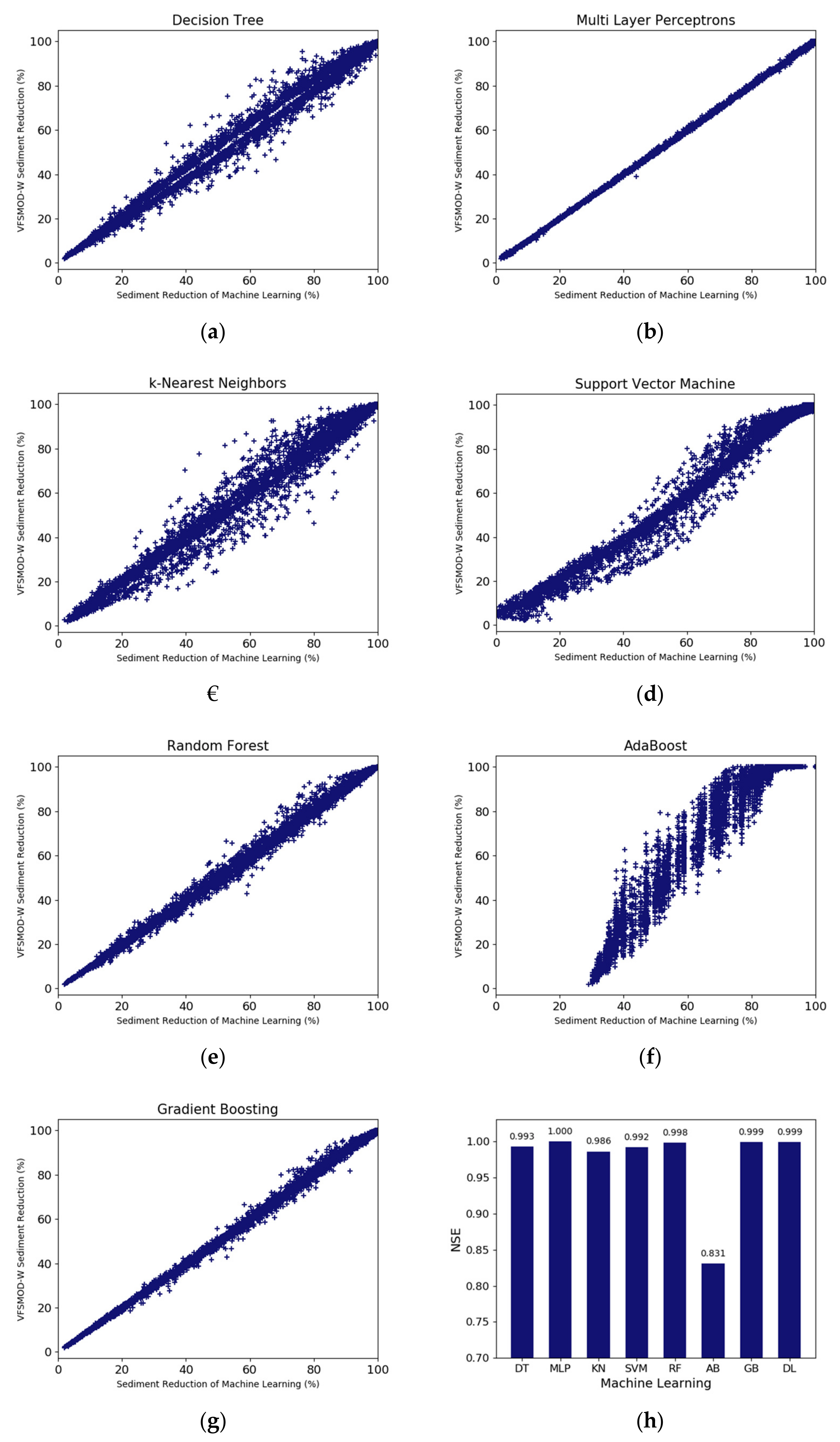
Overall, the machine learning models tested in this study were highly successful in replicating the results of the VFSMOD-W simulations across a wide range of conditions.

Table 11. Prediction accuracy results of seven machine learning models.

Method	NSE	RMSE (%)	MAPE (%)
Decision Tree	0.993	2.15	2.09
Multilayer perceptron	1.000	0.37	0.53
k-Nearest Neighbors	0.986	3.02	2.89
Support Vector Machine	0.992	2.29	2.97
Random Forest	0.998	1.30	1.18
AdaBoost	0.831	10.78	21.81
Gradient Boosting	0.999	0.89	0.78

shows prediction accuracy results (NSE, RMSE and MAPE) of seven machine learning models compared to the sediment trapping efficiencies of VFSMOD-W. The results from MLP and gradient boosting models showed high prediction accuracy indicating MLP with NSE of 1, RMSE of 0.37% and MAPE of 0.53% and gradient boosting with NSE of 0.99, RMSE of 0.89% and MAPE of 0.78%. Thus, these two models would be suggested in this study. MLP and gradient boosting are the most powerful and widely used models in supervised learning and appear to have led to high accuracy by adjusting the hyperparameters using the hidden layers of MLP and the depth of the gradient boosting [27,36].

The results of this analysis show a large overall variation in the success of the machine learning models tested against the VFSMOD-W simulation results. Among the seven machine learning models, AdaBoost showed the lowest performance with NSE of 0.83, RMSE of 10.78% and MAPE of 21.81% as the boosting tends to focus on misclassified samples (data) Also, because the boosting is too dependent on training data, it was too easy to overfit depending on the training data, indicating a rather low accuracy [41]. However, other machine learning models (e.g., decision trees, KNN, SVM and random forest regression models) all showed high performance above 0.98. Using these machine learning models, it is expected that the similar results of sediment trapping efficiencies in VFS can be estimated well.

The most successful machine learning approach tested here was the MLP model. The test data were used to calculate the sediment trapping efficiencies of each machine learning model and the efficiency values calculated in the VFSMOD-W were compared to the efficiencies estimated by machine learning models (Figure 2a–g). Figure 2a–g shows that the sediment trapping efficiency calculated by the MLP regression model is most similar to that of VFSMOD-W. Figure 2h shows a bar graph for easy comparison of NSE of seven machine learning models, which indicates that the results of MLP, gradient boosting and random forest are excellent. Especially MLP has the best results among the seven machine learning models. Since single perceptron classification can be performed with only one straight line, it cannot solve the problem that cannot be divided into straight lines. In MLP, however, it is possible to bend the line by creating a hidden layer. Thus, more flexible prediction can be carried out, and since the hidden layer consists of three layers with 50 nodes each, it is more flexible to predict the sediment trapping efficiency.

The AdaBoost model showed the most different result from the sediment trapping efficiency calculated by VFSMOD-W, and NSE was 0.82. The gradient boosting regression model increased NSE to 0.999 by changing ‘max_depth’ to 10 than the gradient boosting regression model was estimated with the fixed hyperparameter, and it can be seen that the hyperparameter setting can increase the predictive performance. However, when looking at the correlation distribution with the result of VFSMOD-W, the gradient boosting is slightly more distributed than MLP.

As shown in the results, it was found that not only is certain machine learning superior, but also there would be a more suitable model (in terms of prediction) according to the data characteristics, and that the predictive performance can be sufficiently increased by the setting and tuning of hyperparameters.

3.2. Validation of Machine Learning Models

Seven machine learning models were developed in this study to calculate the sediment trapping efficiency of VFS, and the models were validated that the sediment trapping efficiencies can be easily and conveniently calculated without using a physically-based hydrological model, such as VFSMOD-W. However, it is necessary to verify how well the seven machine learning models can predict the sediment trapping efficiency of VFS in real situations.

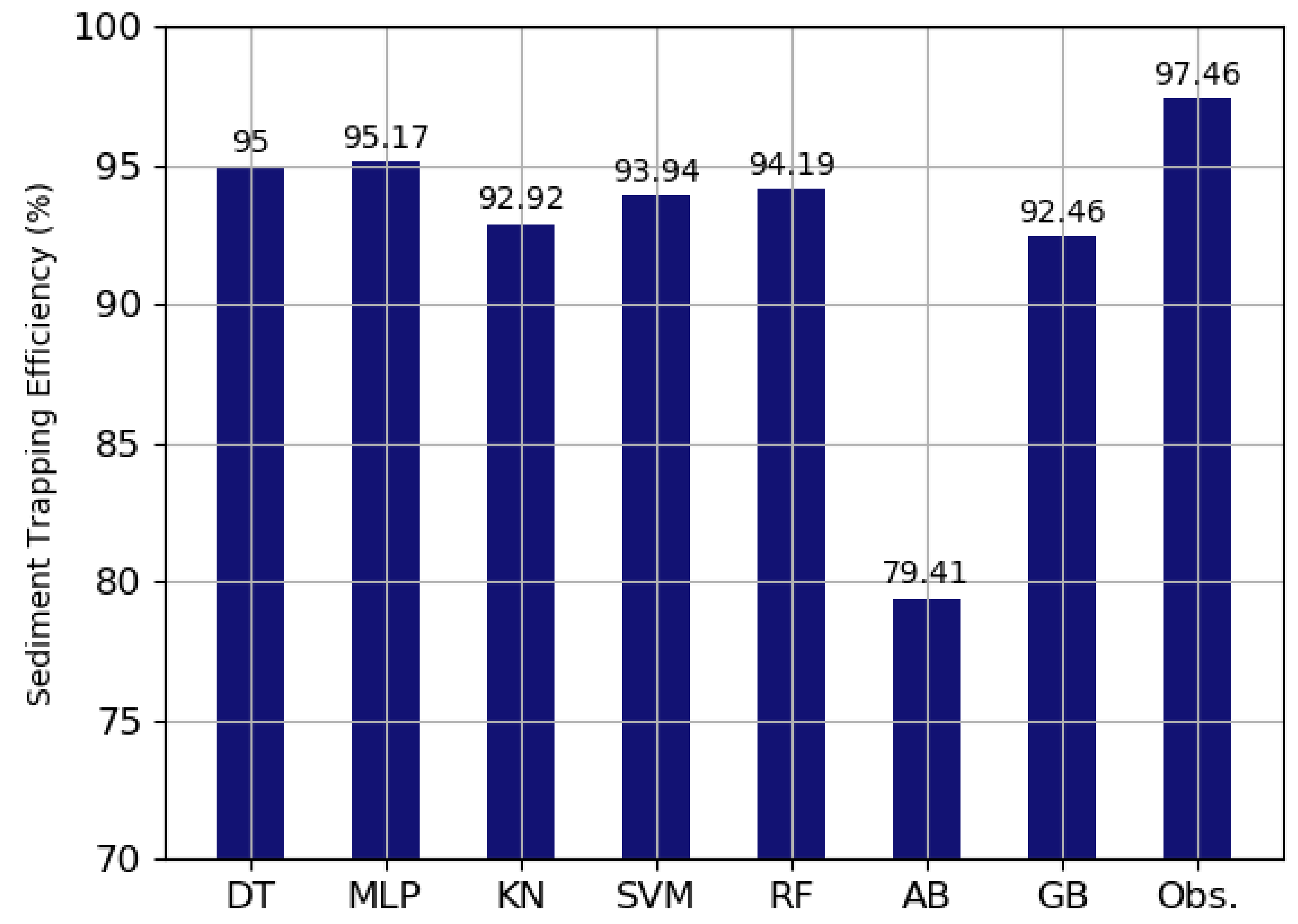
The observations in VFS from the literature review were used to apply the actual situation, and all the machine learning models developed in this study were applied. The study area of VFS in Barfield et al. [44] is a naturally formed karst watershed area. As the input data for the machine learning models, the rainfall was 63.5 mm/hr, and soil texture was specified as loam. The slope was 9%, the area ratio of VFS to a field size was 4.8%, field area was 0.001 ha, the USLE P-factor was 1.0, the USLE C-factor was 0.3, and the CN was 74. The sediment trapping efficiencies predicted in the machine learning models were compared with the observations from Barfield et al. [44] (Figure 3).

The validation results showed MLP and the decision tree were reliable and useful models. Figure 3 showed that the sediment trapping efficiencies calculated by the decision tree, MLP, KNN, SVM, random forest, AdaBoost, gradient boosting were 95%, 95.17%, 92.92%, 93.94%, 94.19%, 79.41%, 92.46%, respectively, and actual sediment trapping efficiency indicated 97.46% which was most similar to the result from MLP and decision tree. The prediction results of MLP and the decision tree showed a percentage error between actual observations and the two models ranged from 2.34 to 2.52%. Thus, the two models (i.e., MLP and the decision tree) are verified as robust models.

3.3. Data Analysis to Develop Machine Learning Models

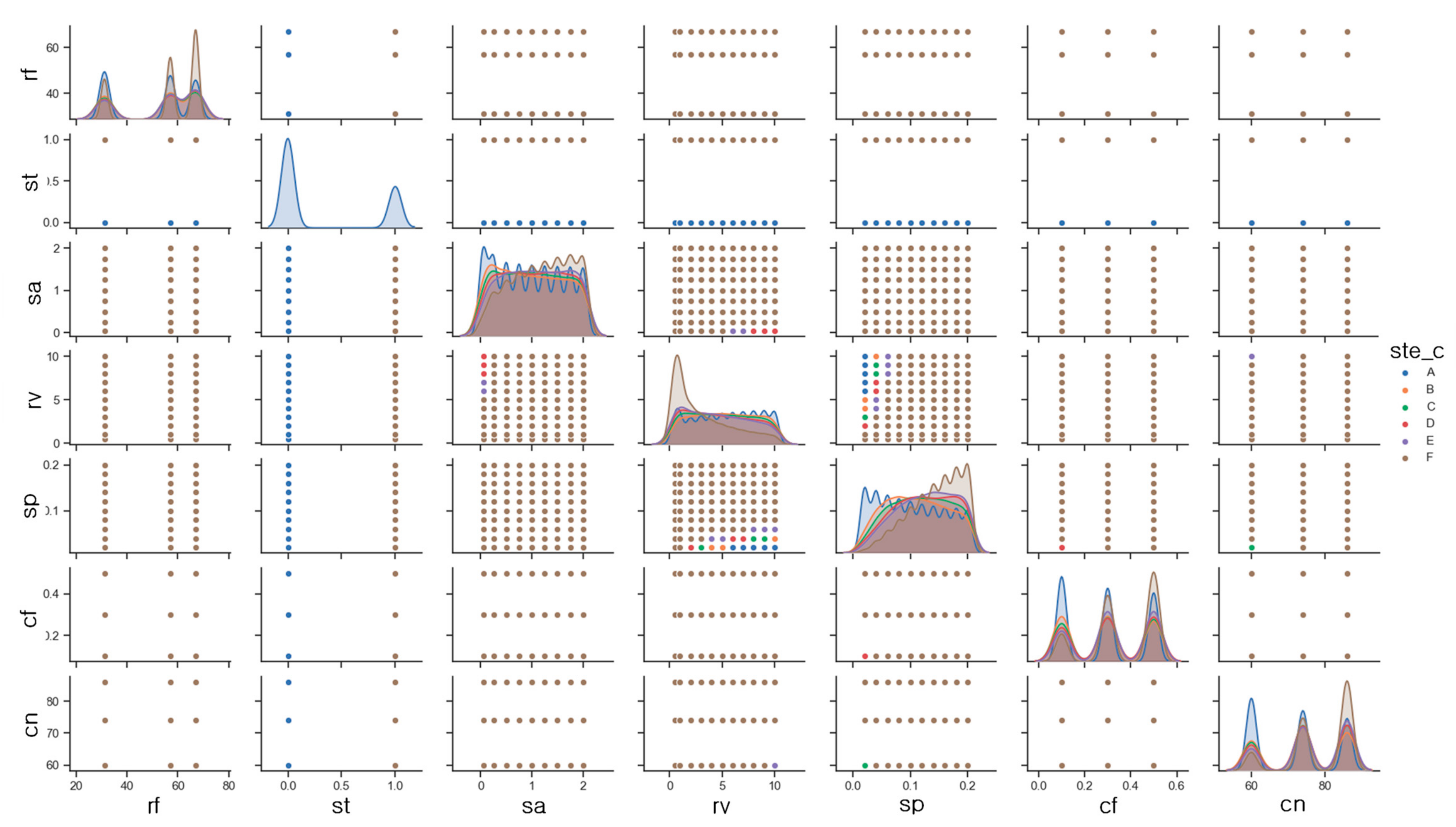
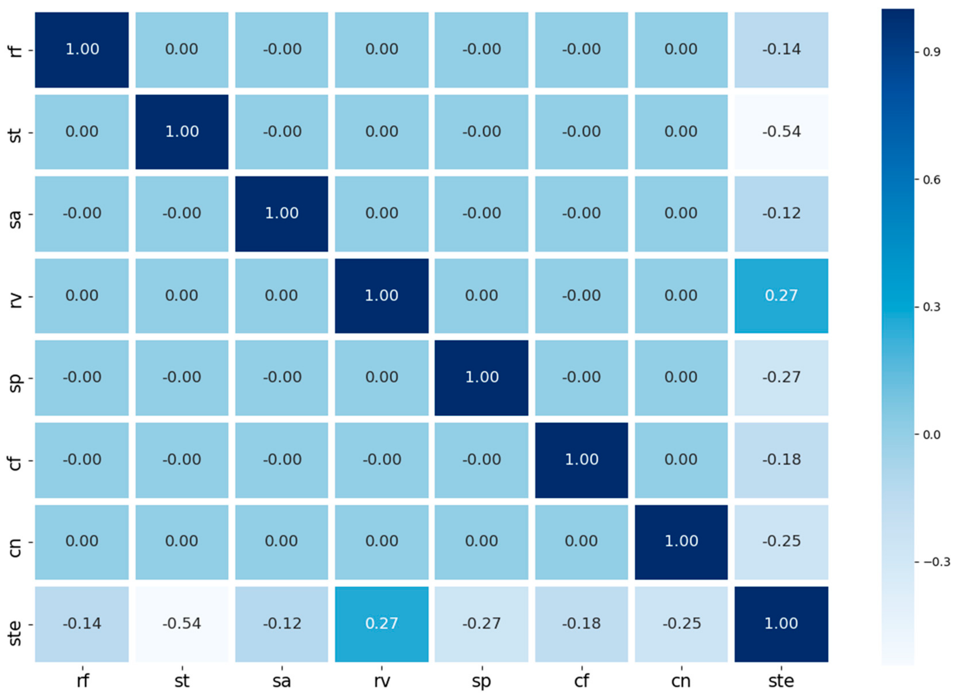
Many parameters related to VFS were used to develop machine learning models. For the development of machine learning models in an effective way, parameters for machine learning models should be analyzed and understood. Using a scatter plot matrix and heat map, correlation analysis between sediment trapping efficiency and model attributes (i.e., rf [rainfall], st [soil texture], sa [source area], rv [ratio of VFS area to source area], sp [slope], cf [USLE C-factor], cn [curve number] and ste [sediment trapping efficiency]) were analyzed. Soil texture (st), the ratio of VFS area to source area (rv) and slope (sp) indicated a strong relationship with sediment trapping efficiency. Figure 4 is a scatterplot matrix which shows that the sediment trapping efficiency and the correlation between each property at the same time. It is expected that Figure 4 can improve readability by presenting the legend in a categorical form with the sediment trapping efficiency. The sediment trapping efficiency category (ste_c) of VFS is assigned as A for more than 90% of the sediment trapping efficiency, B for 80–90%, C for 70–80%, D for 60–70% and E for 50–60%. If the sediment trapping efficiency is less than 50%, we specify an F category value, and we can see the correlation between these categories and each attribute and the histogram of each attribute (Figure 4). The results showed that A and F classes were distributed mostly with 86.7% of the total, and the frequency of B ~ E classes with the remaining 13.3% was low. The class is randomly assigned, so it may be a good idea to take a look at the scattering matrix repeatedly by resetting the sensitively changing classes.

In the scatter plot matrix, it is necessary to look at the histogram of each property. Because the specified attribute values are categorical data rather than continuous data, the distribution also shows a normalized distribution around each category. When the rainfall (rf) is 67 mm, the result shows the sediment trapping efficiency class (ste_c) is mostly F class, whereas, at 31 mm, it shows the highest grade distribution. Through these results, it can be estimated that the more rainfall, the lower the sediment trapping efficiency.

According to Figure 4 and Figure 5, there is a positive strong relationship between the ratio of VFS area to source area (rv) and sediment trapping efficiency. The more rv, the higher the sediment trapping efficiency. This explains that bigger areas of vegetation developed to remove sediment work better for sediment trapping efficiency. The F class is densely distributed in the small VFS to agricultural field area ratio, and the A grade is distributed variously over the entire interval. In the case of the slope (sp), the distribution of the F class is high when the slope is high, and the distribution of the A grade is high in the low slope region. In the case of other attributes, it can be seen that all categories show various classes, and the correlation with the sediment trapping efficiency can be analyzed in the upper distribution.

In the end, however, it is difficult to quantify the correlations only by looking at the correlation between the properties and the sediment trapping efficiency class of VFS. Therefore, the correlation between each input data, including the sediment trapping reduction (ste) of VFS which is continuous numerical data was analyzed using a heat map (Figure 5). Soil texture played a major role in controlling sediment trapping efficiency. The heat map shows that the soil texture (st) of VFS has the strongest influence on the sediment trapping efficiency (ste) with −0.54, and The VFS area ratio (rv) is 0.27 with a positive correlation and the slope (sp) has a negative correlation of −0.27. The sediment trapping efficiency (ste) was statistically significant in the paired T-test results from each attribute (p < 0.001). Multicollinearity does not occur when there are strong correlations between independent variables (Table 2).

3.4. Sensitivity Analysis of Model Hyperparameters

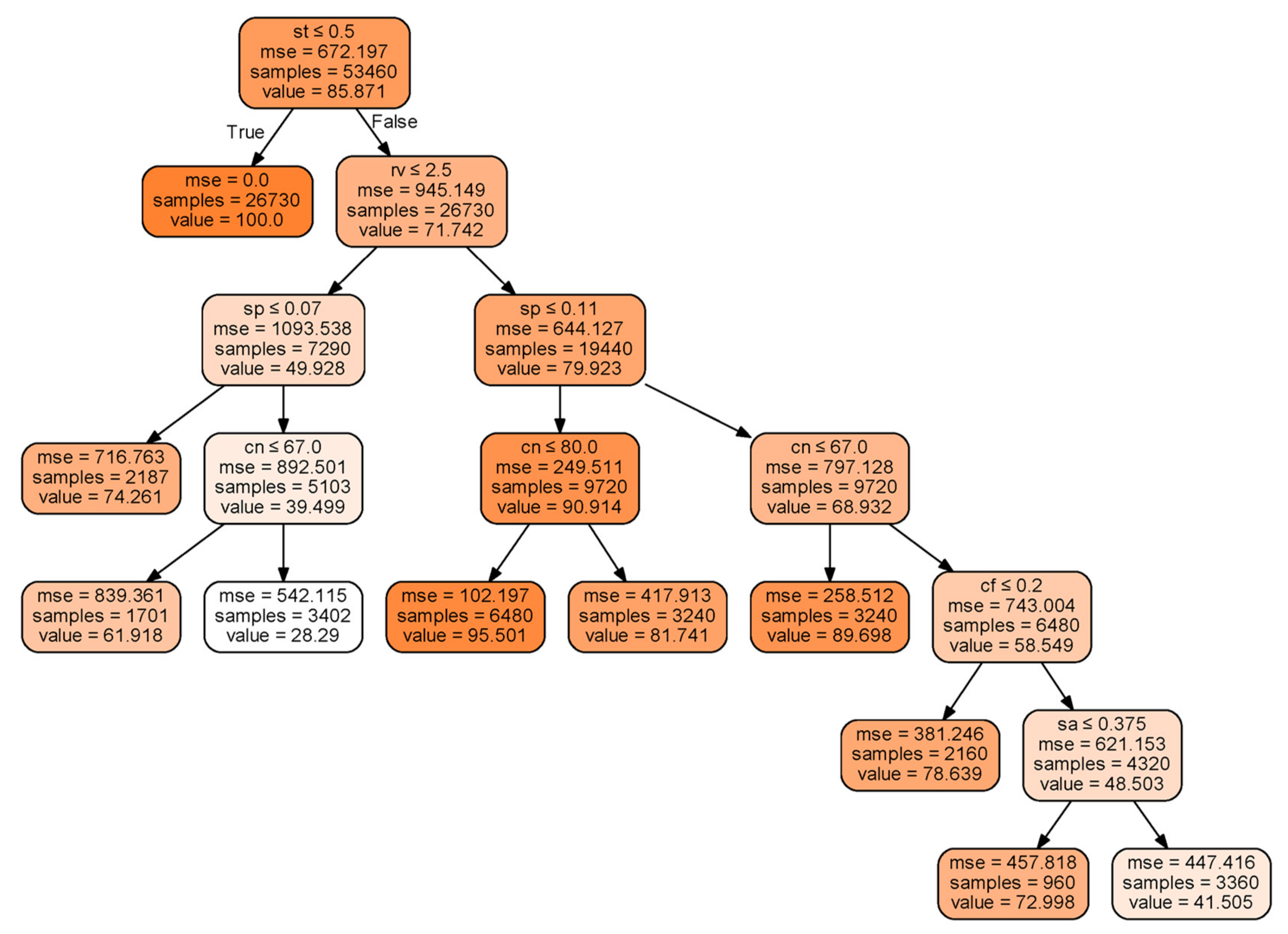
In the seven machine learning regression models, experiments were conducted to set the critical hyperparameters proposed by Müller and Guido [27]. Figure 6 examines how the decision tree method is used to predict the sediment trapping efficiency of VFS. If the maximum number of branches of the decision tree is not determined, a huge distribution with many branches is created. Therefore, in this study, the maximum number of branches (max_leaf_nodes) is set to 10. The mean squared error, which is the classification condition, was calculated to generate a decision tree diagram.

The decision tree diagram is not about predicting the class of data, but rather about the process of predicting consecutive numeric values. As shown in the decision tree diagram, the most influential attribute is soil texture (st), which is the first to be classified in the decision tree classifier. If the criterion of soil texture is less than 0.5, it is classified as true only if it is sandy loam. The next is classified whether the VFS area ratio (rv) is less than or equal to 2.5. If the VFS area ratio (rv) is true, the classification is made under the condition that the slope (sp) is 0.07 or less. As such, it is helpful to understand a decision tree regression based on the criteria of classification.

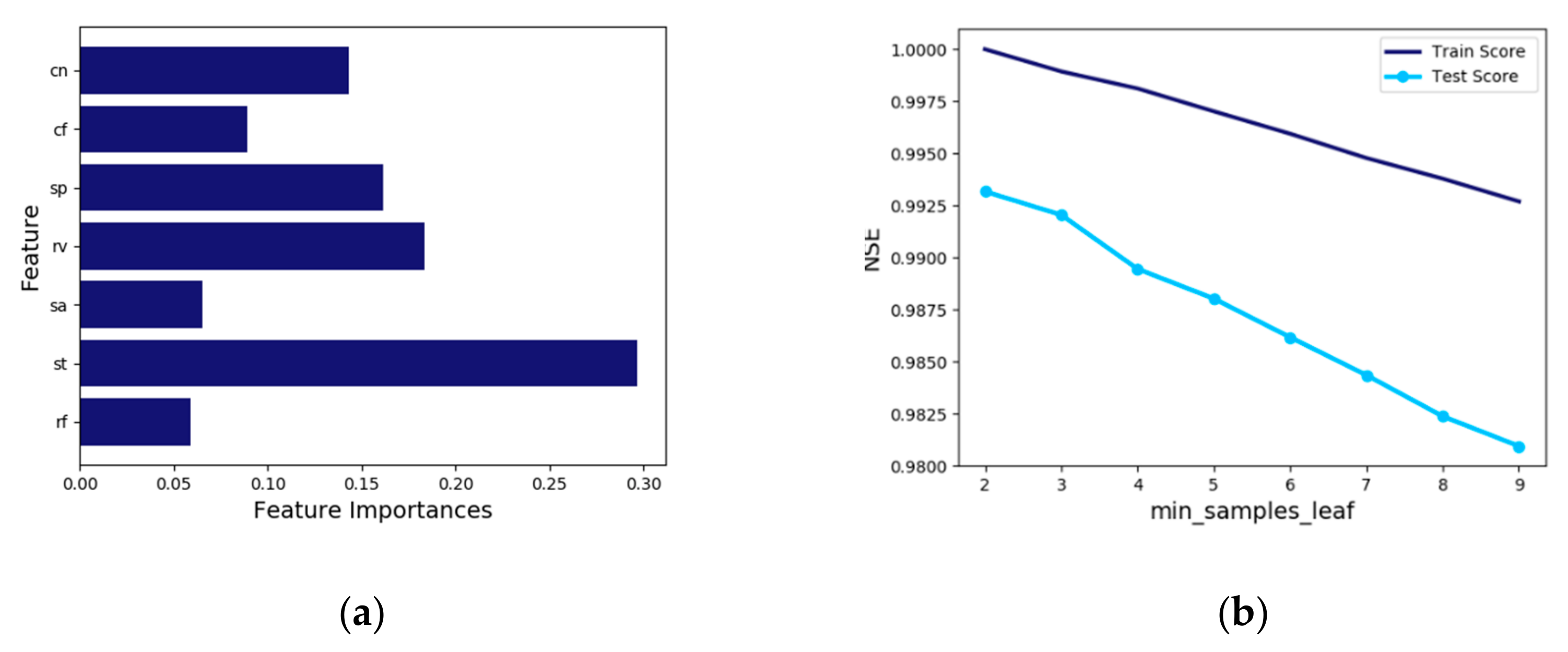
In addition, the influential components are presented in Figure 7a. The most influential property is soil texture (st) which is 0.30. Then, the VFS area ratio (rv) is 0.18, and the third important property is the slope (sp) which is 0.16. This result indicates the same as the order of the decision tree diagram in Figure 6.

Determining the minimum number of samples required to be at a leaf node (Min_samples_leaf) was conducted to prevent overfitting in the regression function (Figure 7b). When ‘min_samples_leaf’ is 2, the best learning is achieved, and the NSE (coefficient of determination) for test is 0.993. This hyperparameter value stops the tree before the decision tree is completely built by pre-pruning. If ‘min_samples_leaf’ goes over 2, the result shows a tendency to sharply decrease in accuracy.

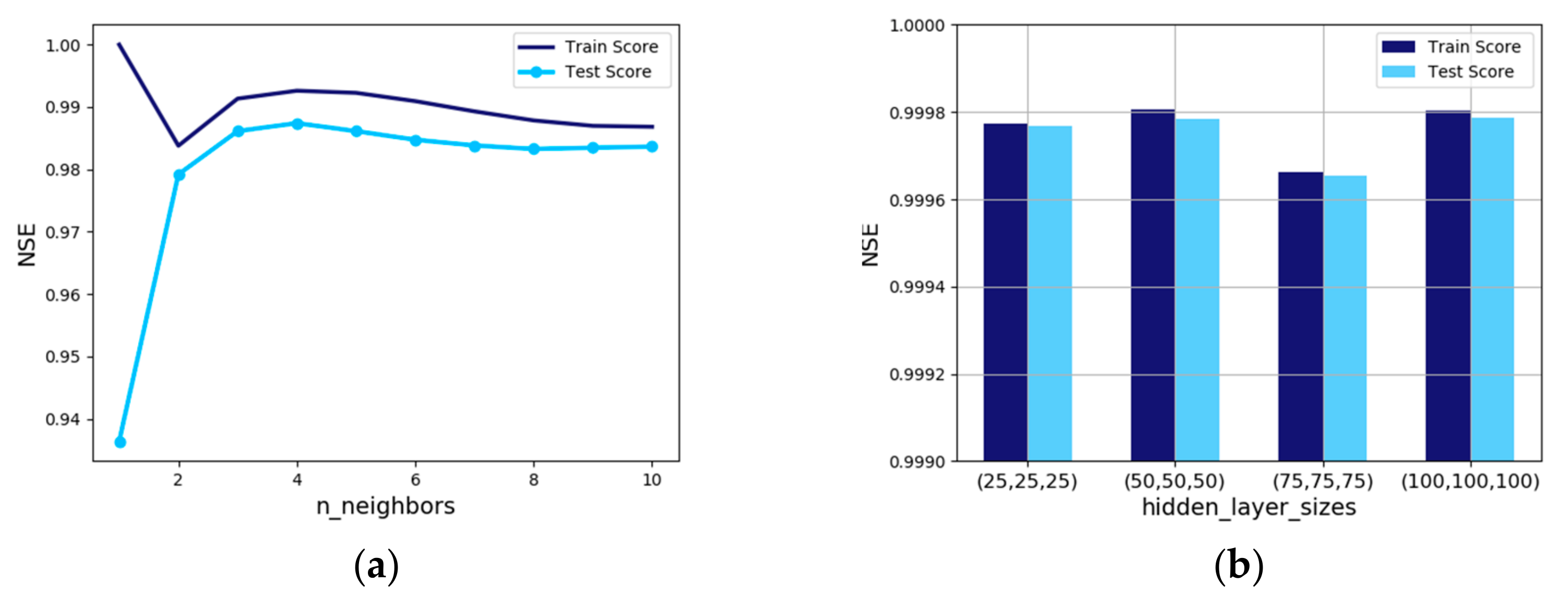
In the k-nearest neighbors model, the use of a large number of neighbors usually does not fit well with the training data, but tends to yield more stable predictions which are a way to prevent overfitting [36]. Therefore, it is important to determine the optimal number of neighbors in the k-nearest neighbors model. Figure 8a indicates that when four neighbors were used, both the training and test show the best results, and the test result shows NSE of 0.987.

An important hyperparameter in the multilayer perceptron regression model (MLPRegressor) is the hidden layer size. In this study, various tests to determine the optimal hidden layers and nodes were conducted, and the results of the four cases are represented in Figure 8b. The best results were obtained by setting three hidden layers with 50 nodes and hyperparameters were set to the same hidden layer and node size.

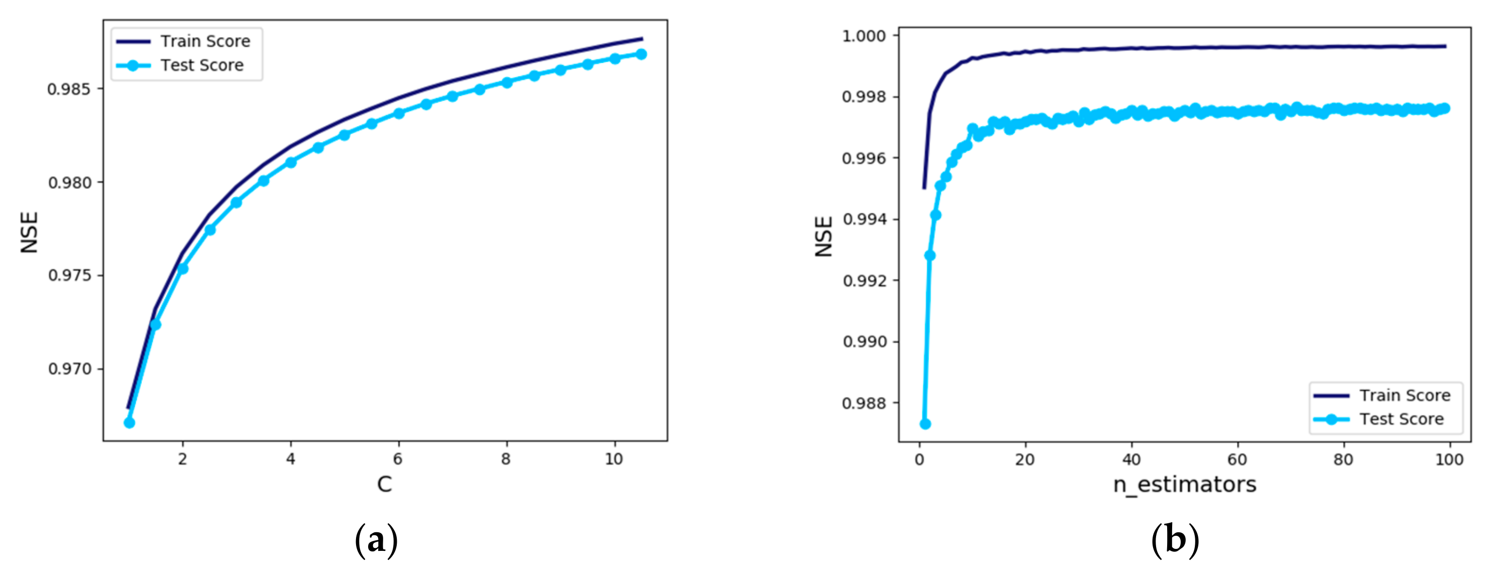
In the support vector machine regression model, a C value was set to 50 because when NSE showed 0.992 in the test data, a C value was 50 (Figure 9a). Since the accuracy of the model increases as the C value increases, the C value is set large. C values determine how many data samples are allowed to be placed in different classes. Lower C values increase the likelihood that there are outliers to find a general decision boundary, while higher C values narrow the likelihood of outliers and more precisely determine the decision boundary. Increasing the C value as much as possible for the fine decision boundary showed good results. In this study, the C value was set to 50, considering calculation speed and overfitting issues.

In order to get the best results of ‘n_estimators’ which is tree numbers and is the sensitive hyperparameter in the random forest regression model, we experimented with varying the settings from 1 to 100. In the case of the test data, no significant change was observed from 20 or more, but the maximum value was set to 52 in this model because the tree number 52 showed an NSE of 0.998 which resulted in the best results (Figure 9b).

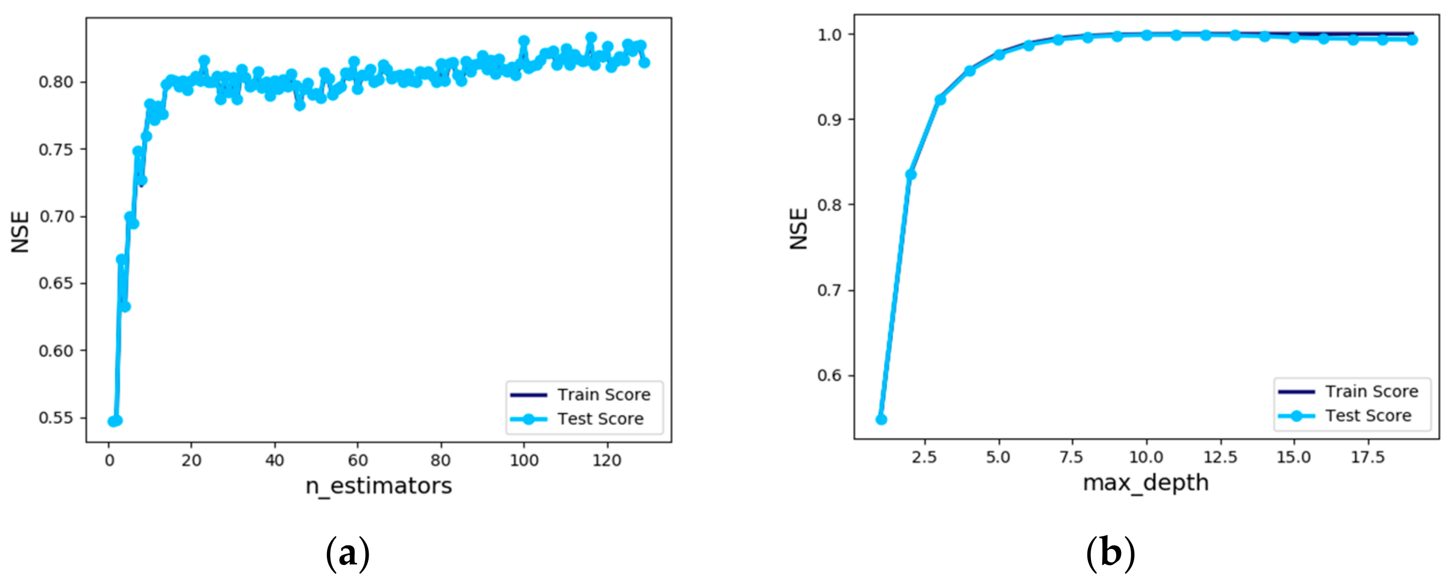
Sensitivity analysis of “n_estimators”, a hyperparameter of the AdaBoost Regressor, was performed. To obtain the most accurate model, the analysis of “n_estimators” was carried out by changing the value from 1 to 129, and the training and test data results showed almost the same trend. When “n_estimators” was validated using the test data, the result showed NSE of 0.831 with 126 learners. Therefore, ‘n_estimators’ of 126 would be appropriate (Figure 10a). In the case of AdaBoost, it is necessary to adjust the ‘learning_rate’ because it shows somewhat lower accuracy by only tuning “n_estimators”. However, the learning rate is adjusted by showing the best NSE of 0.804 at 0.4 and 1 of ‘learning_rate’. The result shows that the accuracy increase cannot be expected greatly. In future studies, it is necessary to study how to produce better results by constructing various combinations of hyperparameters rather than adjusting only a couple of independent hyperparameters.

The critical hyperparameters in the gradient boosting regression model (GradientBoostingRegressor) are ‘n_estimators’ which specify the number of trees and ‘learning_rate’ which compensates for errors in the previous tree [36]. These two parameters are so closely related that lowering ‘learning_rate’ requires adding more trees to create a model of similar complexity.

Sensitivity analysis of two hyperparameters was conducted, and because of the accuracy of up to 0.95, no good results are comparable to MLP. Sensitivity analysis was also carried out by changing the depth of ‘max_depth’ which reduces the complexity of the tree. Setting the value of ‘max_depth’ to 10 increased the accuracy of the gradient boosting regression model, and NSE of the test data was 0.999.

Usually, setting the ‘max_depth’ value to 5 does not make the tree deeper in the gradient boosting model. However, for the data used in this study, it was not unreasonable to use this value to derive the maximum accuracy of the gradient boosting model when the depth value was changed to 10 (Figure 10b).

4. Conclusions

The fundamental objective for estimating the sediment trapping efficiency by VFS is to protect water quality and soil environment. We consider that machine learning is a feasible alternative method of VFSMOD-W to evaluate VFSs efficiently. The machine learning models developed in this study can readily provide robust estimates within the domain of the training and validation data with the appropriate data processing.

For the optimal machine learning model generation, a sensitivity analysis was conducted first to determine most sensitive hyperparameters, and the models were developed by tuning the hyperparameters that were trained and validated in each model through sensitivity analysis. A total of seven machine learning models were tested herein, such as decision tree, MLP, KNN, SVM, random forest, AdaBoost and gradient boosting. The MLP model showed the best results with NSE of 1, RMSE of 0.37% and MAPE of 0.53%, followed by gradient boosting, random forest, decision tree, SVM, KNN and AdaBoost models. Also, all models showed good results with NSE above 0.83.

A particular model is not considered to be superior, and it is possible to improve the learning ability in each model according to the user parameter setting of the algorithm in the model (i.e., the hyperparameter tuning). The results showed that using the appropriate data processing, as well as the training and validation of the model is very important to build robust machine learning models.

In order to build great potential machine learning models to create readily applicable VFSMOD-W models, a couple of further studies is needed. First, impact of data processing (e.g., data pre- and post-processing) and various validation techniques (e.g., k-fold cross validation, leave-one-out cross validation [LOOCV] and bootstrapping) on the accuracy of machine learning models need to be tested. Second, various input data combinations (e.g., soils, land use/land cover, climate, management and topographic information) should be applied to the global extent.

Machine learning models developed in this study can evaluate sediment trapping efficiency without complicated physically-based model design and high computational cost. Thus, machine learning models would be popular among decision makers, such as developers, planners, engineers, local units of government, and decision makers can maximize the quality of their outputs by minimizing their efforts.