Investigating Dominant Trip Distance for Intercity Passenger Transport Mode Using Large-Scale Location-Based Service Data

Abstract

Intercity transport systems have been plagued by low efficiency and overutilization for a long time, due to unhealthy competition among multi-transport modes. Hence, this study aims to estimate the dominant trip distance of intercity passenger transport modes to optimize the allocation of intercity passenger transport resources and improve the efficiency of intercity transport systems. Dominant trip distance was classified into two types: Absolute dominant trip distance and relative dominant trip distance; and their respective models were developed using passenger transport mode share functions and fitting curves. Particularly, the big data of intercity passenger transport mode share rate of more than 360 cities in China was obtained using a network crawler and each passenger transport mode share function and their curves were proposed. Furthermore, the dominant trip distances estimation models of intercity passenger transport were developed and solved. The results show that there are significant differences in dominant trip distance between the transport modes. For example, the absolute and relative dominant trip distances of highway are 8–119 km and 8–463 km, respectively, while those of airway are 1594–3000 km and 2477–3000 km, respectively.

1. Introduction

During the past few decades, the interconnection between cities has been increasingly efficient with the process of regional economic integration in China. Thus, intercity transport plays a vital role in city interconnection. However, intercity transport demand is significantly increasing [1,2], thereby necessitating higher efficiency of intercity transport systems. However, intercity transport systems suffer from low efficiency and high utilization due to unhealthy competition among multi-transport modes including highway, railway, and airway [3,4]. Meanwhile, the contribution by waterway is often excluded due to the inaccessibility of inland water systems in China and its extremely low utilization by passengers [5]. Competition among transport modes is mainly reflected in trip cost including time cost, economic cost, etc. [6,7,8,9,10], while the critical factor influencing trip cost is travel distance [11,12,13,14]. Thus, each transport mode has its dominant trip distance, in which the associated mode share is relatively high [15,16,17]. Within the range of the dominant trip distance, the trip cost of the transport mode is lower and passengers prefer it to other transport modes. Therefore, waste and surplus of traffic resources can be avoided by investigating the dominant trip distances of transport modes. This optimizes traffic structure and provides insightful suggestions for the planning and management of intercity multi-transport systems [18].

Several researchers have investigated the correlation between transport mode choice and trip distance, to understand the dominant trip distances of different transport modes [19,20]. However, traditional studies on dominant trip distance mainly relied on questionnaires or surveys. Dyck et al. [21] conducted a questionnaire on the transport mode choice behaviors of 1281 older adolescents (17–18 years old) from secondary schools in East and West Flanders and set the criterion distance for transportation to the school below 8 km for cycling and below 2 km for walking. Meanwhile, Holz–Rau [22] conducted a survey of the transport mode choice of Berlin residents when they go shopping. The results suggested that the usage of cars dramatically increases when the distance is more than 325 m, and the residents seldom chose other transport modes than cars when the distance is more than 650 m. Furthermore, Zhang et al. [23] conducted a questionnaire on transport mode choice behaviors of passengers in Beijing-Hangzhou transport corridor. The results showed that few passengers prefer to travel by highway when the trip distance was more than 1400 km. Meanwhile, no flights for passengers to choose when the trip distance was less than 300 km.

Traffic questionnaires and surveys have low response efficiency and are costly and time-consuming. It is difficult to obtain datasets with sufficient samples covering various areas or urban agglomerations, thereby limiting large-scale investigation. Therefore, traditional studies only focus on small areas such as urban transportation and some traffic corridors. Moreover, they generally discuss the characteristics of one or two transport modes. For example, Romάn et al. [24] investigated the competition between high-speed trains with air transport using a mixed revealed preferences (RP) and stated preferences (SP) database of Madrid-Barcelona corridors. Ahern et al. [25] examined the perceptions and preferences of passengers to identify the factors that influence the mode choice between bus and train on intercity trips. Furthermore, Cattaneo et al. [26] investigated the role of air transport services in the selection of universities by national students. The results revealed that air transport service affected university choice for long-distance students living at least 300 km from the university. This shows that long or super long trip distances are more applicable to airways.

Several studies have identified transport modes from global positioning system (GPS) trajectories with the increasing availability of GPS. Xu et al. [27] proposed a fuzzy approach by selecting four speed-related fuzzy variables to characterize five transport modes (walk, bike, bus, rail, and rest) in the daily traffic of urban areas. The GPS travel data covering 142 days were obtained automatically from GPS position records carried by 32 volunteers in Shanghai. Gong et al. [28] developed a geographic information system (GIS) algorithm that automatically processes the data from GPS-based travel surveys and detects five travel modes (walk, car, bus, subway, and commuter rail) from a multimodal transportation network in New York City. Additionally, Xiao et al. [29] described the interaction between features that influence transport mode choice using a Bayesian network. They distinguished five representative transport modes (walk, bike, e-bike, bus, and car) using the resulting Bayesian network. Although trip distance can easily be calculated with GPS trajectories, it is difficult to investigate the dominant distances of transport modes based on GPS data due to low data coverage. For individuals, few people can use GPS service uninterruptedly due to its high requirement for mobile networks and hardware. For example, it is difficult to obtain the trajectory of passengers traveling by air because passengers are prohibited from using electronic equipment during flight. Thus, it is unrealistic to use GPS data for large-scale research, as most studies were based on artificial travel experiences [30,31,32].

With the recent popularity of smartphones and online social media platforms, location-based service (LBS) systems such as Google Places, Facebook, Tencent, and Baidu are widely used in several fields including transportation [33,34,35,36]. Rashidi et al. [37] confirmed the applicability of social media data for modeling daily travel behavior, based on the results of a qualitative survey. Zhang et al. [38] proposed a sequential model-based clustering method to group high-resolution Twitter locations and extract Twitter displacements, thereby showing the application of social media data in predicting the travel behavior of individuals. Furthermore, they suggested that social media data is less expensive in comparison with conventional household travel surveys as it is easier to obtain and, most importantly, it can monitor the longitudinal travel behavior features of an individual over a longer observation period. Abbasi et al. [39] analyzed the travel pattern of tourists, using appropriate Twitter information such as the places they visited, travel origin, and destination.

However, past studies mostly focused on the optimization of urban traffic structure due to severe traffic congestions in the city and few intercity trips. Although LBS data has been widely used in urban traffic and has made several achievements [40,41,42,43], few studies exist on dominant trip distances in intercity transportation [44,45]. It’s worthy to mention that existing studies mainly focus on dedicated transport corridor and describe how to get the travel learn from the previous research, trip information including trip distance and trip trajectory can be deduced based on LBS data. Furthermore, transport mode use and share can be obtained based on the previous records of passenger transport hub including airports, railway stations, bus stations, toll gates, etc. In this way, a new database of intercity passenger transport mode share is available for further study. Comparing this database with the database originating from the questionnaire, this database has three advantages: (i) It covers a wide area including a large number of inter-city traffic in different cities and contains more comprehensive transport modes; (ii) it has a high timeliness which can provide both previous data and the latest data; and (iii) it provides more abundant individual travel information.

The primary contribution of this study is the development of dominant trip distance models for intercity passenger transport modes and quantitative analysis of their dominant trip distances using LBS data. More specifically, this study (a) uses a web crawler to download massive LBS data which can facilitate the investigation of the dominant trip distances of intercity passenger transport modes, thereby avoiding the limits of traditional questionnaire; (b) compares intercity multi-transport modes including highway, railway, and airway based on their respective dominant trip distances, thereby improving the previous studies that focused on single transport modes; (c) classifies the dominant trip distances into absolute dominant trip distance and relative dominant trip distance. Two kinds of dominant trip distance models are then developed with LBS data to obtain the dominant trip distance values of highway, railway, and airway in multi-transport systems. The results of this study can guide the rational allocation of intercity transport resources and the positive competition among transport modes, thereby optimizing and improving the efficiency of traffic structures in intercity transport systems.

This study is organized as follows: Section 2 describes the data sources. Section 3 introduces the definition of dominant trip distance and proposes a dominant trip distance model. Section 4 solves the model based on data and discusses the results. Finally, Section 5 concludes and gives the scope for further research.

2. Data

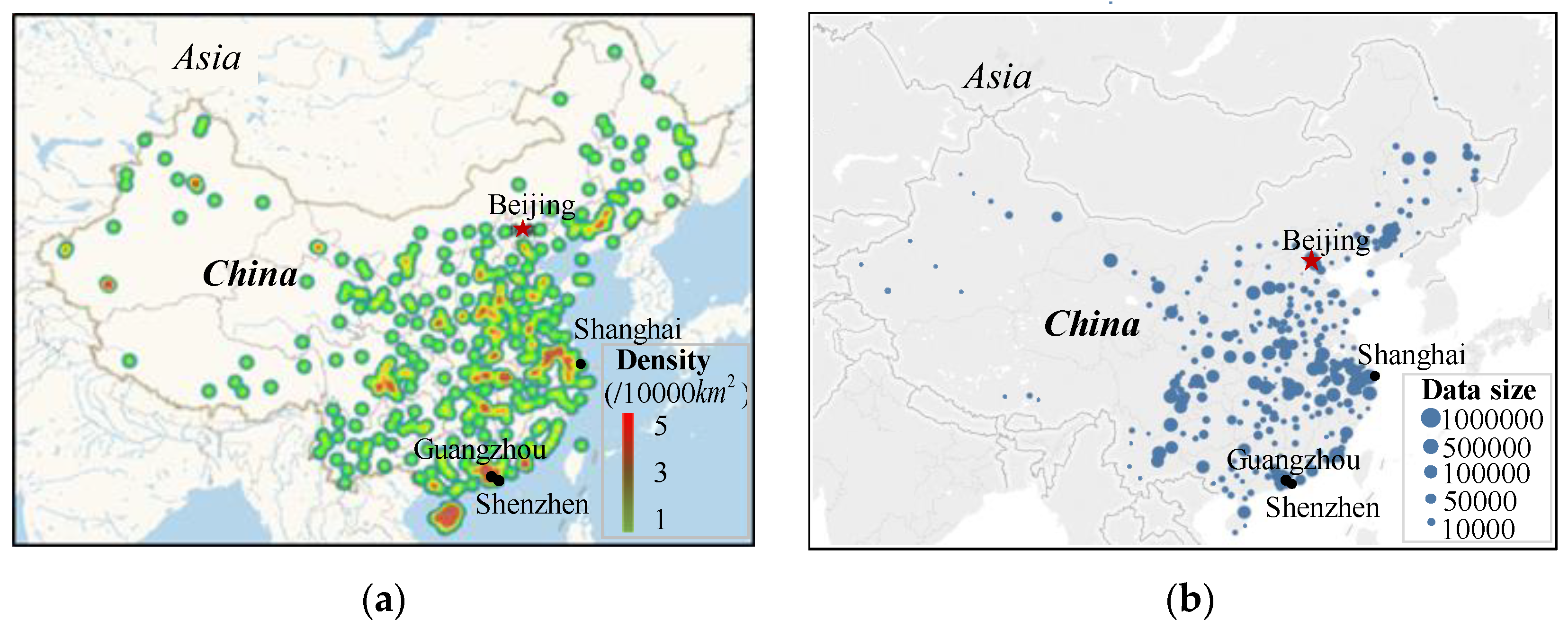
2.1. Data Collection

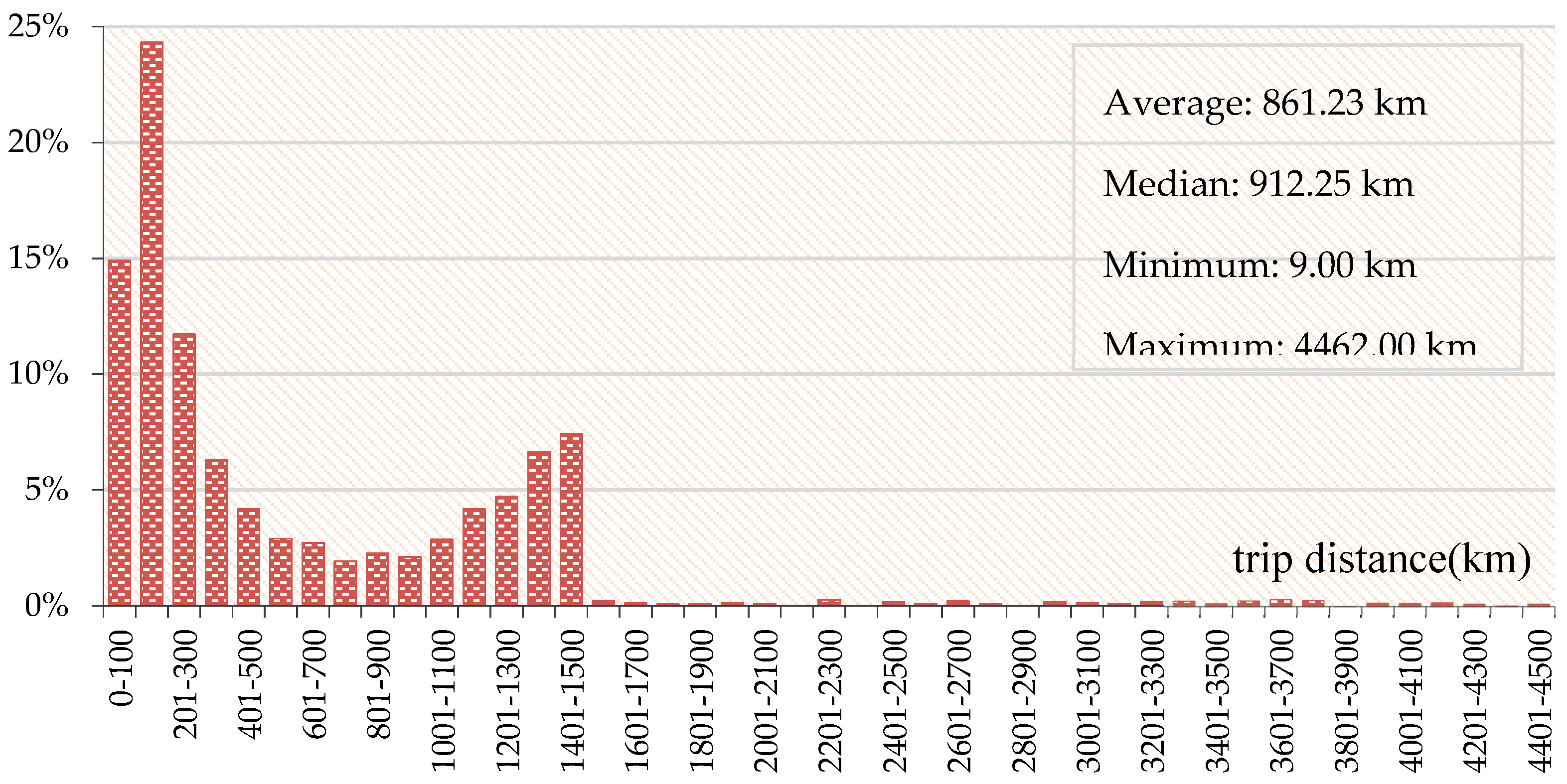
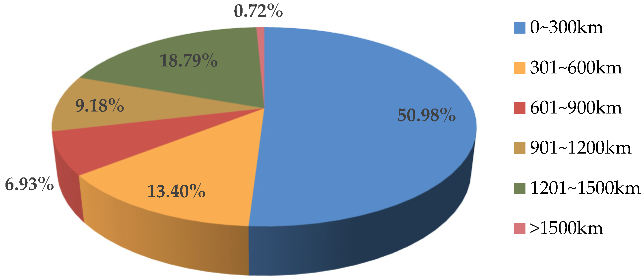
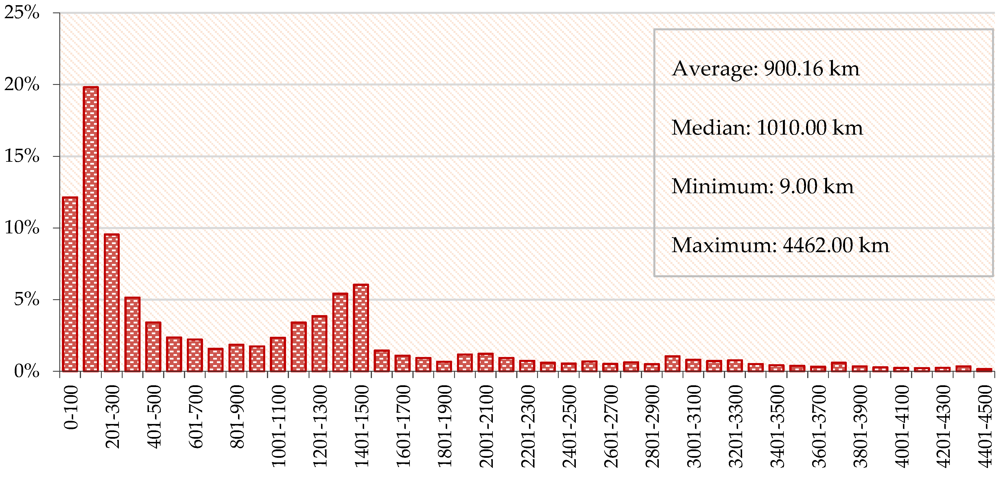
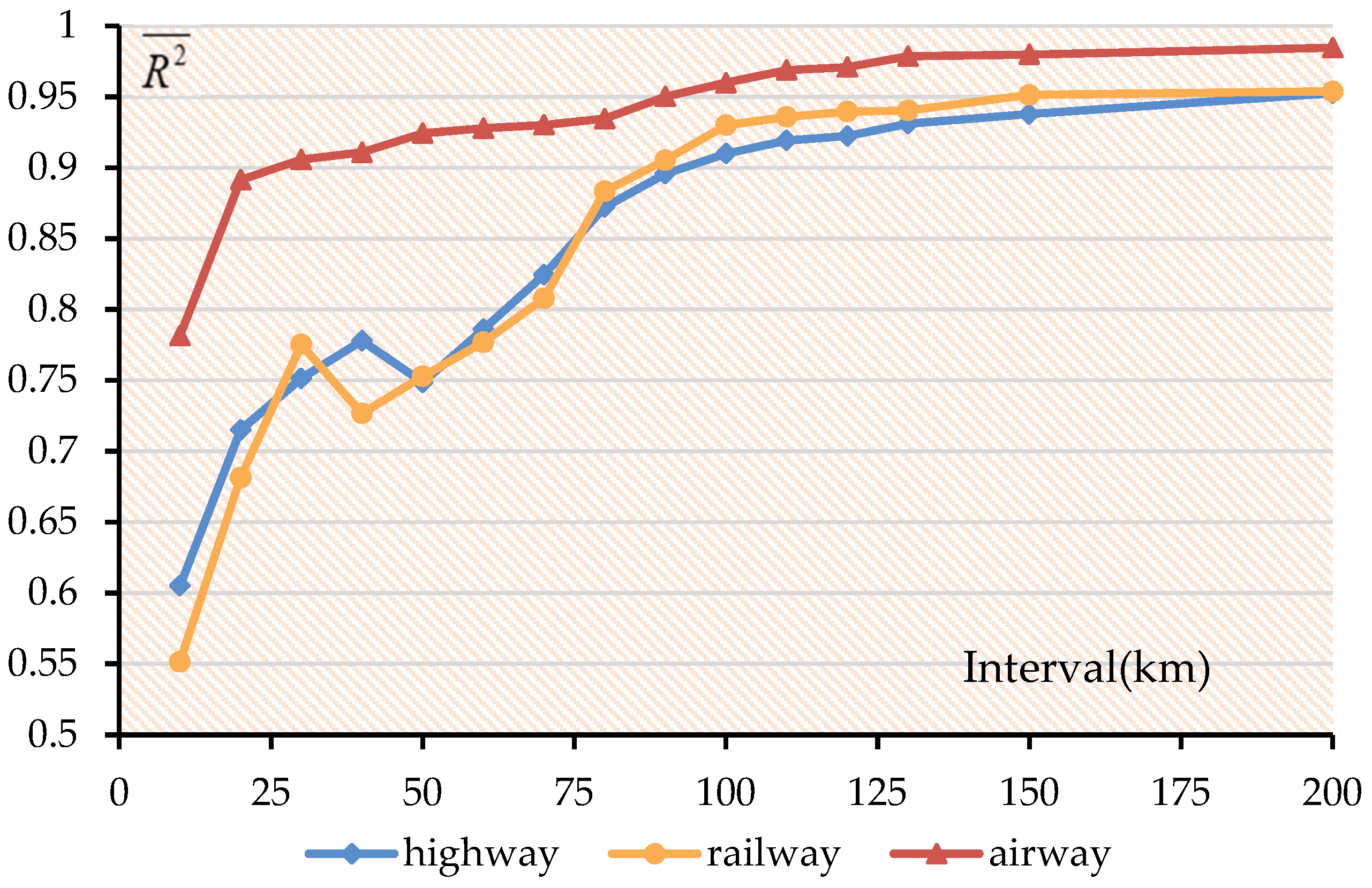
With the development of mobile communication technology and the popularity of smartphones, the real-time location information of mobile phone users can be obtained through location-based services (LBS) provided by kinds of mobile APP. This study used a network crawler to obtain data from https://heat.qq.com/qianxi.php, which is a big data location platform established by Tencent. Presently, this platform can receive more than 60 billion global positioning requests per day, covering one billion users and more than 150 countries worldwide. It provides a new database for research in many fields, such as urban transport, intercity transport, population migration, etc. In addition, the platform provides users with a search bar, which can be used to input city name and date. Mode share between two cities since February 3rd, 2015 is freely available to obtain.

The platform can store previous historical locations of travelers when receiving positioning requests and then calculate their trip distances. Moreover, the transport mode of travelers can be identified through the appearance records of trip speed and key passenger transport hubs such as bus stations, train stations, and airports. Then, each traveler’s transport mode is concluded. Finally, the mode share data of various intercity passenger transport modes can be obtained, which is significant to investigations in intercity transport structures and dominant trip distances of transport modes.

In this study, Python 3.6 was set as the development environment, and a web crawler was coded using Selenium programing library. Furthermore, BeautifulSoup and SimpleJson programming libraries were used to parse the web while the data was downloaded and stored in a data center using Pandas. Additionally, the data format was converted into an appropriate format and stored in a local file. The data acquisition process is shown in Figure 1.

In this study, 125 days of travel data in 2017 was collected, in which more than 25 days of data were recorded in each season including data of National Day Golden Week, Spring Festival, and other special periods. Moreover, 663,780 data records including date, departure city, destination city, and mode share of transport modes were obtained.

Table 1. Dataset of mode share in intercity transport.

No.	Date	Departure	Destination	Highway Mode Share	Railway Mode Share	Airway Mode Share
1	1 October 2017	Beijing	Chongqing	1%	30%	69%
2	1 October 2017	Beijing	Shanghai	13%	42%	45%
3	1 October 2017	Beijing	Changsha	0%	53%	47%
…	…	…	…	…	…	…
10	1 October 2017	Beijing	Zhengzhou	11%	87%	2%
11	1 October 2017	Chongqing	Beijing	0%	28%	71%
12	1 October 2017	Shanghai	Beijing	13%	39%	48%
13	1 October 2017	Wuhan	Beijing	10%	63%	27%
…	…	…	…	…	…	…
20	1 October 2017	Tianjin	Beijing	27%	73%	0%
…	…	…	…	…	…	…

shows the data table.

Meanwhile, no information about distance was obtained, which is essential for studies on the dominant trip distances of the transport modes. Considering the road distance, railway distance, and air distance between two cities are different. Thus, the distance D between the cities was calculated based on the longitude and latitude of each city obtained from Google Maps. The calculation formula is given by Equation (1):

$$D=2R·arcsin\left(\sqrt{si{n}^2\left(\frac{la{t}_a-la{t}_b}{2}\right)+cos\left(la{t}_a\right)·cos\left(la{t}_b\right)·si{n}^2\left(\frac{lo{n}_a-lo{n}_b}{2}\right)}\right)$$

(1)

where $la{t}_a$ and $lo{n}_a$ represent latitude and longitude of departure city, respectively; $la{t}_b$ and $lo{n}_b$ represent latitude and longitude of destination city, respectively; and R represents radius of the Earth, unit: Kilometer; D represents the distance between two cities, unit: Kilometer.

The data obtained include 361 departure cities and 362 destination cities, covering all regions of China. The city distribution is shown in Figure 2, where regions shown in red have dense urban agglomerations and regions shown in green have sparse urban agglomerations. From the perspective of city distribution, cities in eastern and southern coastal areas are denser, which is consistent with the development of regional economy in China.

2.2. Data Analysis

Based on existing research, trip distance has a significant impact on the choice of transport modes by travelers. To clarify the distance distribution, all distances were classified at the interval of 100 km. The number of each type of data was then counted, and the proportion of each type was calculated, as shown in Figure 3. The most common trip distance range of intercity transport in China is 101–200 km. Moreover, trip distance ranges of 8–100 km and 201–300 km had large proportions. When trip distance is within 100–800 km, the proportion decreased gradually with the increase of trip distance. However, when trip distance is greater than 800 km, the proportion increased gradually to 1500 km. Subsequently, there was a sharp decline, especially after 1500 km, such that the proportion of trips for these distances was extremely low. The reason is that the announced data from big data platform of Tencent covers daily information of each transport mode of the cities ranked by the top ten cities in China’s 365 cities. Specifically, such data contain city name, data, the mode share of intercity passenger transport between a specific city and the other cities, etc. For instance, as shown in Table 1, when Beijing is the departure city, Chongqing, Shanghai, Changsha, …, and Zhengzhou are the top ten cities as destination for intercity passenger volume generation. Meanwhile, when Beijing is the destination city, Chongqing, Shanghai, Wuhan, …, and Tianjin are the top ten cities as departure for intercity passenger volume attraction. The distances between cities whose passenger volumes rank top ten are mostly within 1500 km, therefore, there is an abrupt difference between 1401–1500 km and 1501–1600 km.

Based on the above classification, the trip distances were classified again according to the interval of 300 km. However, data with distances greater than 1500 km were merged into one group, considering the low proportion. Figure 4 shows the pie chart of the distribution. Intercity passenger travel in China is dominated by short distance, which is less than 300 km. This accounts for more than half of the total passenger volume. Meanwhile, mid-distance travel also accounts for a large proportion of the total passenger volume, while long-distance travel over 1500 km accounts for a very low proportion (0.72%). Hence, regional travel in China mainly focuses on short and medium distances.

Considering that the proportion of long-distance trip data is extremely small, it is necessary to supplement the data to ensure the accuracy of subsequent data analysis. As a result, a second data acquisition was performed from the same platform to maintain data consistency. We collected all currently published data when trip distance is greater than 1500 km and randomly selected a date and collected travel records with distances within 500–1200 km, considering their overall proportions is too small to make subsequent data analysis. Finally, 274,484 data records whose trip distances are within 500–1200 km and 80,000 data records whose trip distances are over 1500 km were obtained and supplemented with the datasets. Finally, 1,016,064 data records were obtained, including 17,132 different urban O-D pairs. However, the number of each type of data also was counted, and the proportion of each type was calculated, as shown in Figure 5. The final trip distance distribution bar diagram is shown in Figure 5. The minimum distance between cities was 9.00 km, and the maximum distance was 4662.00 km, covering a wide range of distance. Moreover, the average distance between cities was 900.16 km.

3. Methodology

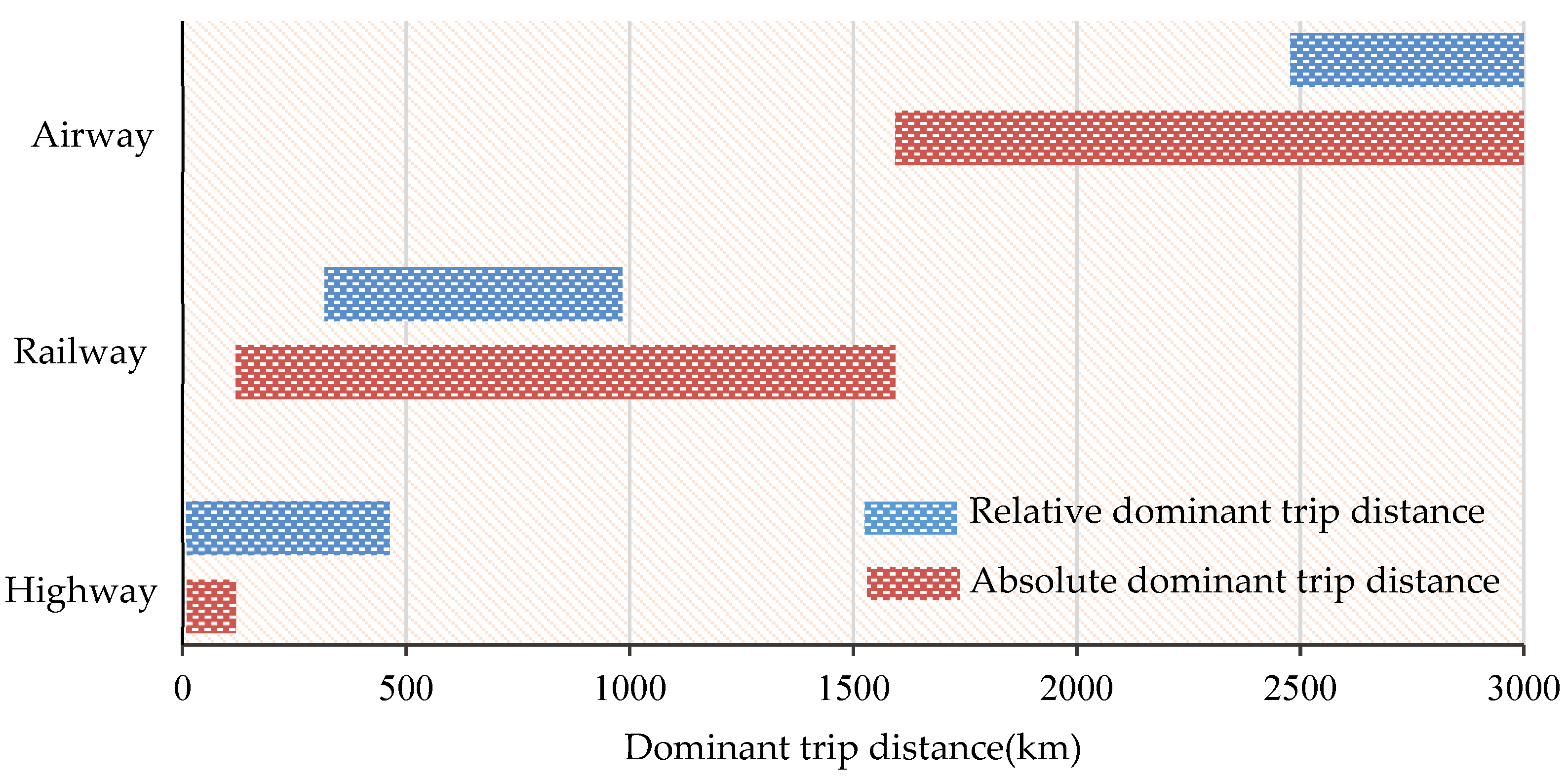
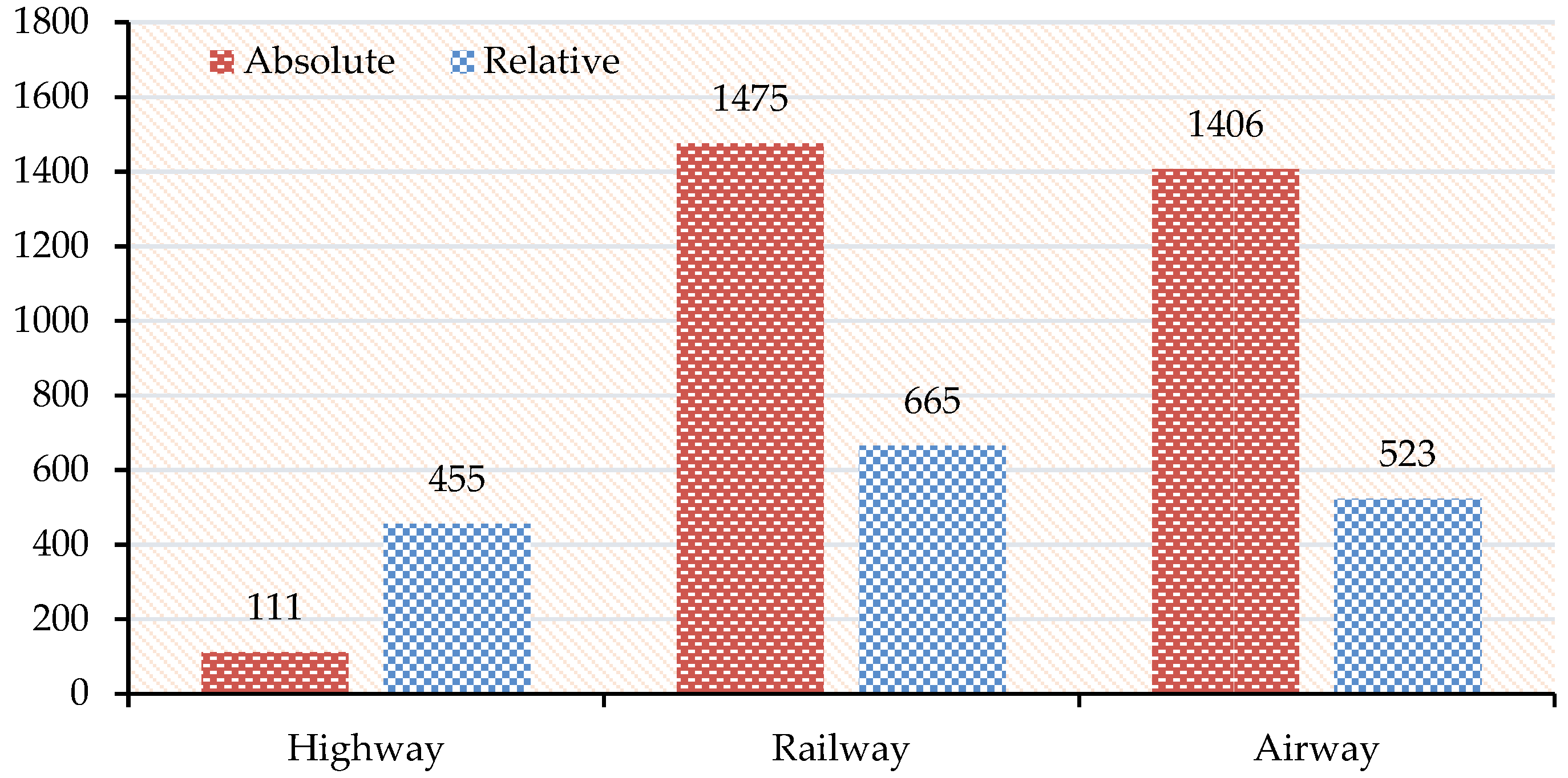
3.1. Dominant Trip Distance Definition

There are similarities between passenger transport and freight transport in the study of dominant trip distance. Thus, the dominant trip distance of passenger transport mode is divided into two categories: Absolute dominant trip distance and relative dominant trip distance, by referring to the classification of dominant freight transport distance [46]. The definitions are given as follows:

• Absolute dominant trip distance—This is the trip distance range where the mode share value of a passenger transport mode is greater than that of any other passenger transport mode.
• Relative dominant trip distance—This is the trip distance range where the mode share value of a passenger transport mode in a certain trip distance range is greater than that of any other trip distance range of the same distance.

3.2. Modeling of Absolute Dominant Trip Distance

Based on the definition of absolute dominant trip distance of passenger modes, a model can be constructed as shown in Equation (2):

$$\{\begin{array}{c}{f}_i\left(k\le x\le l\right)>f_j\left(k\le x\le l\right)\\ i\ne j\\ i,j\in 1,2,3\\ \alpha \le k\le \beta \\ \alpha \le l\le \beta \\ k\le l\end{array}$$

(2)

where $f_i\left(x\right)$ and $f_j\left(x\right)$ represent the mode share of a type of transport mode when trip distance is $x$ km, $i$ and $j$ = 1, 2, 3. The values of $f_1\left(x\right)$, $f_2\left(x\right)$, and $f_3\left(x\right)$ represent the mode share of highway, railway, and airway respectively; $k$ and $l$ represent the value of trip distances (km); $\left[\alpha ,\beta \right]$ represents the trip distance range covering all trips. The absolute trip distance range $\left[k,l\right]$ can be obtained by solving Equation (2).

3.3. Modeling of Relative Dominant Trip Distance

Based on the definition of the relative dominant trip distance of passenger transport mode, the solution of relative dominant trip distance can be transformed into the solution of minimum distance range when the area of closed figure surrounded by its mode share curve and the distance range is fixed. The minimum trip distance range corresponding to the fixed area is the relative dominant trip distance range of a passenger transport mode. Thus, the model of relative dominant trip distance is given by Equation (3).

$$\begin{gathered} \min d=m-n \\ s.t.\{\begin{array}{c}{{\displaystyle \int }}_n^m{f}_i\left(x\right)dx=\gamma {{\displaystyle \int }}_{\alpha }^{\beta }{f}_i\left(x\right)dx\\ \alpha \le m\le \beta \\ \alpha \le n\le \beta \\ m-n\ge 0 \end{array} \end{gathered}$$

(3)

where $m$ and $n$ represent the value of trip distance (km); $d$ represents the length of relative dominant trip distance range (km); $\mathsf{\gamma }$ represents the dominant coefficient, whose value ranges from zero to one; $\left[\alpha ,\beta \right]$ represents the trip distance range covering all trips and $m$, $n$ are in this range. The value of $m$ and $n$ can be obtained by solving Equation (3). The relative dominant trip distance range is $\left[n,m\right]$.

4. Result Analysis

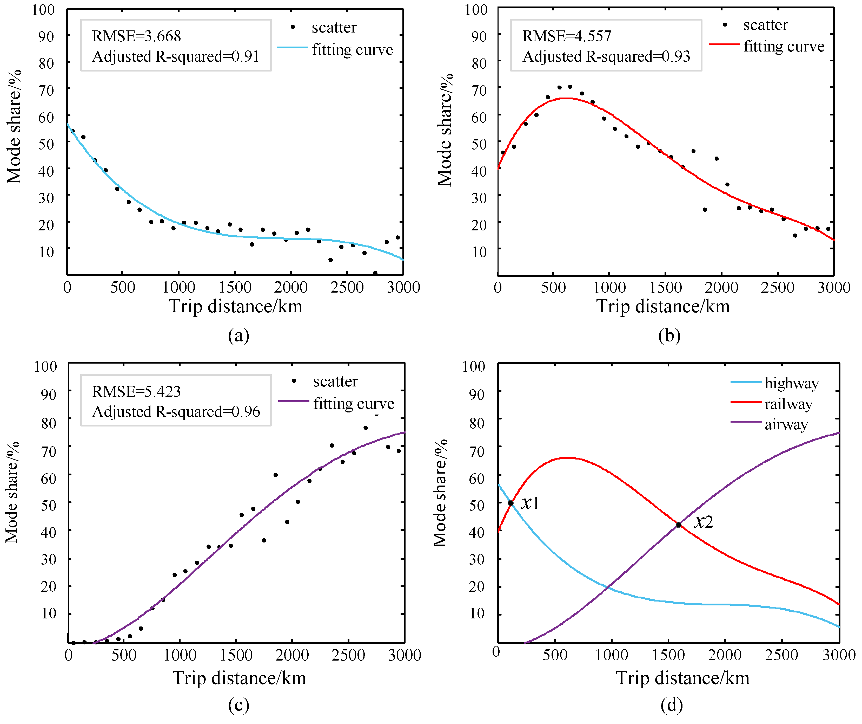
4.1. Mode Share Functions and Curves

The proportion of trips over 3000 km is extremely low such that it is insufficient for data processing. Therefore, data with trip distances greater than 3000 km were excluded in the following steps. Furthermore, data was clustered to reduce the impact of noise, due to the large size of the dataset. After several cluster tests with different interval sizes, the adjusted R- squared values of highway, railway, and airway were stable and kept greater than 0.9 when the particle size was over 100 km, and the values were greater than 0.9, as shown in Figure 6. Therefore, all the data were categorized at a travel distance interval of 100 km. Meanwhile, the average trip distance of each type was represented as $D^{\prime }$. Moreover, the average values of transport mode share in each type were calculated separately and represented as $M_d^{car}$, $M_d^{train}$, $M_d^{air}$. Thus, a new dataset $\left\{M_d^{car},M_d^{train},M_d^{air},D^{\prime }\right\}$ was created.

On the basis of data classification, datasets $\left\{M_d^{car},D^{\prime }\right\}$, $\left\{M_d^{train},D^{\prime }\right\}$, and $\left\{M_d^{air},D^{\prime }\right\}$ were fitted with different statistical distributions including linear distribution, exponential distribution, logarithmic distribution, polynomial distribution, power distribution, and moving average distribution using MATLAB.

Furthermore, two metrics, adjusted R-squared ($\overline{R^2}\overline{R^2}$) and root-mean-squared error (RMSE), were calculated using Equations (4) and (5), respectively, to evaluate the goodness of fit. Figure 6 shows the calculation results. In Equations (4) and (5), $y_i$ represents the real value of the mode share; $\overline{y }$ represents the average value of the mode share; and $\widehat{y_i}$ represents the fitting value. Moreover, n is the number of samples and p is the number of explanatory variables. From Figure 6, ($\overline{R^2}$) is close to one in all fitting functions, which shows that the mode share functions and curves are credible.

$$R_{adjusted}^2=1-\frac{n-1}{n-p-1}\left[1-\frac{{{\displaystyle \sum }}_{i=1}^n{\left(\widehat{y_i}-\overline{y}\right)}^2}{{{\displaystyle \sum }}_{i=1}^n{\left(y_i-\overline{y}\right)}^2}\right]$$

(4)

$$RMSE=\sqrt{\frac{1}{n}{\displaystyle \sum }_{i=1}^n{\left(y_i-\widehat{y_i}\right)}^2}$$

(5)

Table 2. Calculation results of all statistical distributions.

Statistical Distribution Function	RMSE			Adjusted R-Squared
	Highway	Railway	Airway	Highway	Railway	Airway
Exponential	3.333	12.870	5.872	0.936	0.475	0.952
Gaussian	3.059	3.952	5.953	0.942	0.950	0.950
Polynomial	3.668	4.557	5.423	0.914	0.934	0.959
Power	3.831	7.304	5.840	0.912	0.831	0.953
Fourier	4.809	5.495	5.361	0.868	0.904	0.96

shows the calculation results of all the statistical distributions, which indicates that polynomial distribution and gaussian performs better in both R-squared and RMSE. However, polynomial distribution function is much simpler than gaussian distribution function, which is easy to use and understand. Therefore, the following data fitting were all made with polynomial distribution.

The mode share functions of intercity passenger transport modes were then obtained, based on trip distance denoted as $x$ ranging from eight to 3000 km, as shown in Equation (6)–(8).

Mode share function of intercity highway:

$$f_1\left(x\right)=-5.718\times {10}^{-9}{x}^3+3.321\times {10}^{-5}{x}^2-6.525\times {10}^{-2}x+56.96$$

(6)

Mode share function of intercity railway:

$$f_2\left(x\right)=-5.853\times {10}^{-12}{x}^4+4.527\times {10}^{-8}{x}^3-1.198\times {10}^{-4}{x}^2+0.1015x+39.26$$

(7)

Mode share function of intercity airway:

$$f_3\left(x\right)=\{\begin{array}{cc}\hfill 0\hfill & (0~25 \mathrm{km})\hfill \\ \hfill 1.105\times {10}^{-12}{x}^4-1.11\times {10}^{-8}{x}^3+3.14\times {10}^{-5}{x}^2+1.584\times {10}^{-3}x-2.196\hfill & (250~3000 \mathrm{km})\hfill \end{array}$$

(8)

Furthermore, the mode share curves of transport modes were obtained based on their mode share models, as shown in Figure 7.

From Figure 7a, the highway mode share decreases monotonously as the trip distance increases. When the trip distance is between eight and 300 km, the mode share of highway is over 40%. In long-distance travel where trip distance is close to 3000 km, the highway mode share is 10% or smaller, indicating that highway is suitable for short-and medium-distance travel, especially short-distance travel.

From Figure 7b, the railway mode share increases first and then decreases as trip distance increases. The trip distance corresponding to the inflection point is about 600 km, and the mode share is over 65%. When the trip distance is within 10–1650 km, the railway mode share is more than 40%. This shows that railway has obvious advantages for short, medium, and long distances.

From Figure 7c, the airway mode share decreases monotonously as the trip distance increases. When the trip distance exceeds 1550 km, the airway mode share exceeds 40%, which indicates that airway has advantages for long and super long distances.

Figure 7d combines the passenger sharing curves of highways, railways, and airways. The passenger mode share varies with trip distance, and different passenger transport modes have their own dominant trip distance. Thus, transport structure is the result of competition among the different transport modes based on trip distance.

4.2. Solution of Absolute Dominant Trip Distance

Based on the share rate curve of transport modes, the intersection point of the highway sharing curve and railway sharing curve is set as $x_1$, and the intersection point of the railway sharing curve and airway sharing curve is set as $x_2$, as shown in Figure 7d.

According to the model of absolute dominant trip distance and Figure 7d, when the trip distance ranges from eight to 3000 km:

$$\{\begin{array}{cc}{f}_1\left(8\le x\le x_1\right)\ge f_j\left(8\le x\le x_1\right)& j=2,3\\ f_2\left(x_1\le x\le x_2\right)\ge f_j\left(x_1\le x\le x_2\right)& j=1,3\\ f_3\left(x\ge x_2\right)\ge f_j\left(x\ge x_2\right)& j=1,2\end{array}$$

(9)

Therefore, the absolute dominant trip distance of highway, railway, and airway are $\left[8,x_1\right]$, $\left[x_1,x_2\right]$, and $\left[x_2,3000\right]$, respectively.

The absolute dominant trip distance of intercity passenger transport modes can be estimated by Equation (10) composed of Equations (6) and (7) and Equation (11) composed of Equations (7) and (8). The intersection values of $x_1$ and $x_2$ are solved separately. They satisfy the requirements of $8\le x\le 3000$.

$$\{\begin{array}{c}{f}_1\left(x\right)=-5.718\times {10}^{-9}{x}^3-6.525\times {10}^{-2}x+56.96 \\ f_2\left(x\right)=5.853\times {10}^{-12}{x}^4+4.527\times {10}^{-8}{x}^3-1.198\times {10}^{-4}{x}^2+0.1015x+39.26\\ f_1\left(x\right)=f_2\left(x\right) \end{array}$$

(10)

$$\{\begin{array}{c}{f}_2\left(x\right)=5.853\times {10}^{-12}{x}^4+4.527\times {10}^{-8}{x}^3-1.198\times {10}^{-4}{x}^2+0.1015x+39.26 \\ f_3\left(x\right)=1.105\times {10}^{-12}{x}^4-1.11\times {10}^{-8}{x}^3+3.14\times {10}^{-5}{x}^2+1.548\times {10}^{-3}x-2.196\\ f_2\left(x\right)=f_3\left(x\right) \end{array}$$

(11)

The solution shows that $x_1$ is equal to 119 km and $x_2$ is equal to 1594 km. Therefore, when the trip distance ranges from eight to 3000 km, the absolute dominant trip distance of highway, railway, and airway is 8–119 km, 119–1594 km, and 1594–3000 km, respectively.

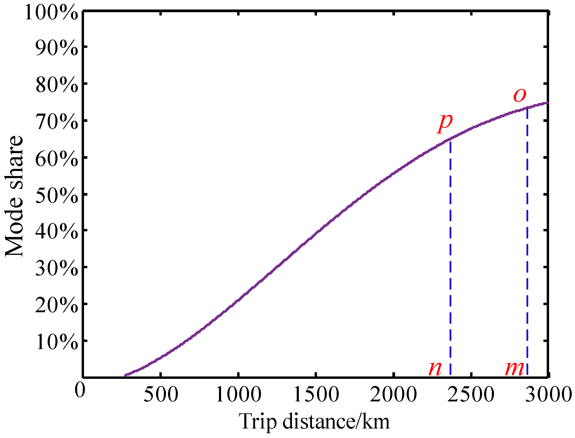
4.3. Solution of Relative Dominant Trip Distance

Based on the model of relative dominant trip distance, the relative dominant trip distance of transport modes varies with the dominant coefficient value. In this study, the dominant coefficient was set to 1/3 as an example, and the relative dominant trip distance can be solved in the following way:

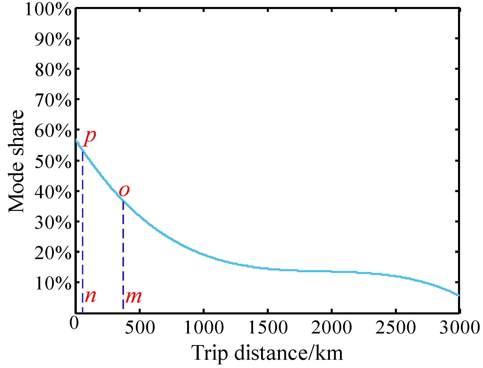
• Relative dominant trip distance of highway—As shown in Figure 8, there are four unknown points $m$ , $n$, $o$, $p$. The values of $m$ and $n$ can be calculated by the area surrounded by $m$, $n$, $o$, $p$ and the highway mode share curve.

The relative dominant trip distance of highway with trip distance range of 8–3000 km is established as Equation (12). The value of $\gamma$ is set as 1/3.

$$\begin{gathered} \min d=m-n \\ s.t.\{\begin{array}{c}{{\displaystyle \int }}_n^m{f}_1\left(x\right)dx=\frac{1}{3}{{\displaystyle \int }}_8^{3000}{f}_1\left(x\right)dx\\ 8\le m\le 3000 \\ 8\le n\le 3000 \\ m-n\ge 0 \end{array} \end{gathered}$$

(12)

The solution shows that $n$ is equal to 8.00 km and $m$ is equal to 463.28 km, indicating that the relative dominant trip distance of highway is 8–463 km, which covers a range of 455 km.

2.

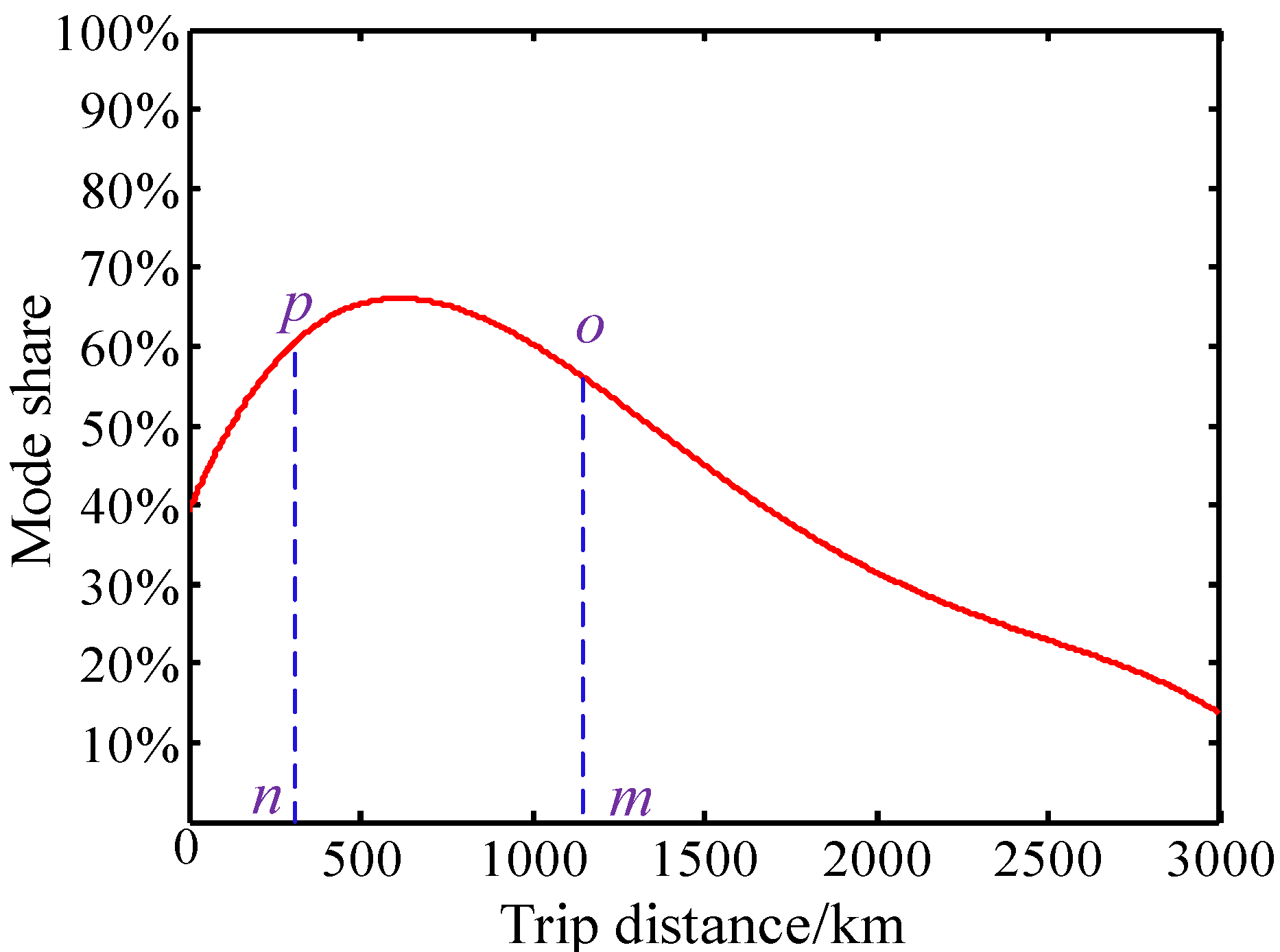
Relative dominant trip distance of railway—As shown in Figure 9, there are four unknown points $m$, $n$, $o$, $p$, and the values of $m$ and $n$ can be calculated by the area surrounded by $m$, $n$, $o$, $p$, and the railway mode share curve.

The relative dominant trip distance of railway with trip distance range of 8–3000 km is given by Equation (13):

$$\begin{gathered} \min d=m-n \\ s.t.\{\begin{array}{c}{{\displaystyle \int }}_n^m{f}_2\left(x\right)dx=\frac{1}{3}{{\displaystyle \int }}_8^{3000}{f}_2\left(x\right)dx\\ 8\le m\le 3000 \\ 8\le n\le 3000 \\ m-n\ge 0 \end{array} \end{gathered}$$

(13)

The solution shows that $n$ is equal to 344.70 km and $m$ is equal to 1043.70 km, indicating that the relative dominant trip distance of highway is 345–1044 km, which covers a range of 699 km.

3.

Relative dominant trip distance of airway—As shown in Figure 10, there are four unknown points $m$, $n$, $o$, $p$, and the values of $m$ and $n$ can be calculated by the area surrounded by $m$, $n$, $o$, $p$, and the airway mode share curve.

The relative dominant trip distance of airway with trip distance range of 8–3000 km is given by Equation (14):

$$\begin{gathered} \min d=m-n \\ s.t.\{ \begin{array}{c}{{\displaystyle \int }}_n^m{f}_3\left(x\right)dx=\frac{1}{3}{{\displaystyle \int }}_8^{3000}{f}_3\left(x\right)dx\\ 8\le m\le 3000 \\ 8\le n\le 3000 \\ m-n\ge 0 \end{array} \end{gathered}$$

(14)

The solution shows that $n$ is equal to 2,476.50 km and $m$ is equal to 3000 km, indicating that the relative dominant trip distance of airway is 2477–3000 km, which covers a range of 523 km.

Therefore, when the trip distance ranges from eight to 3000 km and the dominant coefficient is set as 1/3, the relative dominant trip distance of highway, railway, and airway are 8–463 km, 345–1044 km, and 2477–3000 km, respectively.

4.4. Result Analysis

In this study, the relative dominant trip distance and absolute dominant trip distance of highway, railway, and airway within 8–3000 km were obtained by modeling with LBS data, which are shown in

Table 3. Dominant trip distance range of intercity passenger transport modes.

Transport Mode	Absolute Dominant Trip Distance	Relative Dominant Trip Distance
highway	8–119	8–463
railway	119–1594	318–983
airway	1594–3000	2477–3000

and Figure 11.

The absolute dominant trip distance of highway is 8–119 km and its relative dominant trip distance is 8–463 km, which indicates that highway has significant advantages in short and medium trip distances. This is because highway has characteristics of convenience, moderate speed, and high cost. However, long-distance trips by cars are often time-consuming and uneconomical. The absolute dominant trip distance of railway is 119–1594 km and its relative dominant trip distance is 318–983 km, which shows that passengers prefer railway when traveling at medium and long distances. This is because railway has characteristics of lower cost and faster speed in comparison with highway. The absolute dominant trip distance of airway is 1594–3000 km and its relative dominant trip distance is 2477–3000 km, which indicates that airway has significant advantages in long and super long distances. This is because airway has the fastest speed. Meanwhile, few passengers prefer airway when traveling at short and medium distances because of its high cost and long waiting time. As the trip distance increases, the advantages of airway gradually emerge.

From the perspective of dominant trip distance range shown in Figure 12, railway has the largest dominant range both in the absolute dominant trip distance and relative dominant trip distance. Airway and highway come next. Meanwhile, there is little difference in absolute dominant trip distance between railway and airway. However, there is a huge gap between highway and the other two modes. From the comparison of the two types of distance, the absolute dominant trip distance ranges of railway and airway are larger than the relative dominant trip distance ranges, while the highway is on the contrary. This indicates that the applicable travel distance of highway is more concentrated.

5. Conclusions

In this study, absolute dominant trip distance and relative dominant trip distance were defined based on the dominant trip distance of passenger transport mode. Furthermore, absolute dominant trip distance model and relative dominant trip distance model were developed based on the transport mode shares, and a method that quantifies and systematically compares the dominant trip distance of transport modes was proposed. Additionally, big data of China intercity transport mode share was obtained using a network data crawler. The mode share functions and curves were then established, based on trip distance. Moreover, absolute dominant trip distance and relative dominant trip distance values of highway, railway, and airway were obtained, based on the proposed models and data.

The results show that transport modes have their dominant trip distance. The absolute dominant trip distances of highway, railway, and airway are 8–119 km, 119–1594 km, and 1594–3000 km, respectively; while their relative dominant trip distances are 8–463 km, 318–983 km, and 2477–3000 km, respectively. Highway has excellent advantages for short-distance trips while railway is mostly preferred in medium-distance trips. When traveling at long and super long distances, passengers usually prefer airway because it takes the least time.

Furthermore, the absolute dominant trip distance and relative dominant trip distance of various traffic modes were quantitatively analyzed. By comparing the dominant trip distance of the transport modes, intercity transport resources can be rationally allocated, thereby avoiding resource surplus or resource shortage, improving the efficiency of intercity transport systems, and promoting the coordinated development of regional integration.

In addition, some shortcomings need to be improved. The dominant trip distance of transport modes is solved based on transport mode shares. However, other factors such as economy, region, holidays, etc., also have an impact on transport mode choice. In the future, we will classify the data based on the factors mentioned and solve the dominant trip distance under different types. Furthermore, the influence of various factors on the dominant trip distance of transport modes will be explored by studying the change of dominant trip distance.

References

1. Baohua, M.A.O.; Quanxin, S.U.N.; Shaokuan, C. Structural analysis on 2008 intercity transport system of China. J. Transp. Syst. Eng. Inf. Technol. 2009, 9, 10–18. [Google Scholar]
2. Carlsson, F. The demand for intercity public transport: The case of business passengers. Appl. Econ. 2003, 35, 41–50. [Google Scholar] [CrossRef]
3. Morton, A.L. Intermodal competition for the intercity transport of manufactures. Land Econ. 1972, 48, 357–366. [Google Scholar] [CrossRef]
4. Oum, T.H.; Gillen, D.W. The structure of intercity travel demands in Canada: Theory tests and empirical results. Transp. Res. Part B Methodol. 1983, 17, 175–191. [Google Scholar] [CrossRef]
5. Liu, B.L.; Liu, Y. Estimation in China Cumulative Amount of Highway and Waterway Capital. J. Beijing Jiaotong Univ. 2007, 3, 44–48. [Google Scholar]
6. Chiou, Y.C.; Lan, L.W.; Chang, K.L. Sustainable consumption, production and infrastructure construction for operating and planning intercity passenger transport systems. J. Clean. Prod. 2013, 40, 13–21. [Google Scholar] [CrossRef]
7. Ivaldi, M.; Vibes, C. Price competition in the intercity passenger transport market: A simulation model. J. Transp. Econ. Policy 2008, 42, 225–254. [Google Scholar]
8. Moeckel, R.; Fussell, R.; Donnelly, R. Mode choice modeling for long-distance travel. Transp. Lett. 2015, 7, 35–46. [Google Scholar] [CrossRef]
9. Lapparent, M.; Axhausen, K.W.; Frei, A. Long distance mode choice and distributions of values of travel time savings in three European countries. Arb. Verk. Raumplan. 2010, 570. Available online: https://doi.org/10.3929/ethz-a-005864249 (accessed on 24 September 2019). [CrossRef]
10. Espino, R.; de Dios Ortúzar, J.; Román, C. Understanding suburban travel demand: Flexible modelling with revealed and stated choice data. Transp. Res. Part A Policy Pract. 2007, 41, 899–912. [Google Scholar] [CrossRef]
11. Müller, S.; Tscharaktschiew, S.; Haase, K. Travel-to-school mode choice modelling and patterns of school choice in urban areas. J. Transp. Geogr. 2008, 16, 342–357. [Google Scholar] [CrossRef]
12. Kim, N.S.; Van Wee, B. The relative importance of factors that influence the break-even distance of intermodal freight transport systems. J. Transp. Geogr. 2011, 19, 859–875. [Google Scholar] [CrossRef]
13. Arbués, P.; Baños, J.F.; Mayor, M.; Suárez, P. Determinants of ground transport modal choice in long-distance trips in Spain. Transp. Res. Part A Policy Pract. 2016, 84, 131–143. [Google Scholar] [CrossRef] [Green Version]
14. Scheiner, J. Interrelations between travel mode choice and trip distance: Trends in Germany 1976–2002. J. Transp. Geogr. 2010, 18, 75–84. [Google Scholar] [CrossRef]
15. Zumkeller, D.; Nakott, J. Neues Leben für die Städte. Grünes Licht fürs Fahrrad. Bild Wiss. 1988, 5, 104–113. [Google Scholar]
16. Jiang, F.; Johnson, P.; Calzada, C. Freight demand characteristics and mode choice: An analysis of the results of modeling with disaggregate revealed preference data. J. Transp. Stat. 1999, 149–158. [Google Scholar] [CrossRef]
17. Fan, Q.; Wang, W.; Hua, X.; Wei, X.; Liang, M. Dominant transport distance for multi transport modes in urban integrated transport network based on general travel costs. J. Transp. Syst. Eng. Inf. Technol. 2018, 18, 25–31. [Google Scholar]
18. Kang, Y.S.; Herr, P.M.; Page, C.M. Time and distance: Asymmetries in consumer trip knowledge and judgments. J. Consum. Res. 2003, 30, 420–429. [Google Scholar] [CrossRef]
19. Stead, D.; Marshall, S. The relationships between urban form and travel patterns. An international review and evaluation. Eur. J. Transp. Infrastruct. Res. 2001, 1, 113–141. [Google Scholar]
20. Ewing, R.; Cervero, R. Travel and the built environment: A synthesis. Transp. Res. Rec. 2001, 1780, 87–114. [Google Scholar] [CrossRef]
21. Van Dyck, D.; De Bourdeaudhuij, I.; Cardon, G.; Deforche, B. Criterion distances and correlates of active transportation to school in Belgian older adolescents. Int. J. Behav. Nutr. Phys. Act. 2010, 7, 87. [Google Scholar] [CrossRef] [PubMed]
22. Holz-Rau, H.C. Wechselwirkungen zwischen Siedlungsstruktur und Verkehr: Verkehrsverhalten beim Einkauf. Int. Verk. 1991, 43, 300–305. [Google Scholar]
23. Zhang, J.N.; Zhao, P. Research on passenger choice behavior of trip mode in comprehensive transportation corridor. China Railw. Sci. 2012, 33, 123–131. [Google Scholar]
24. Román, C.; Espino, R.; Martín, J.C. Competition of high-speed train with air transport: The case of Madrid–Barcelona. J. Air Transp. Manag. 2007, 13, 277–284. [Google Scholar] [CrossRef]
25. Ahern, A.A.; Tapley, N. The use of stated preference techniques to model modal choices on interurban trips in Ireland. Transp. Res. Part A Policy Pract. 2008, 42, 15–27. [Google Scholar] [CrossRef]
26. Cattaneo, M.; Malighetti, P.; Paleari, S.; Redondi, R. The role of the air transport service in interregional long-distance students’ mobility in Italy. Transp. Res. Part A Policy Pract. 2016, 93, 66–82. [Google Scholar] [CrossRef]
27. Xu, C.; Ji, M.; Chen, W.; Zhang, Z. Identifying travel mode from GPS trajectories through fuzzy pattern recognition. In Proceedings of the 2010 Seventh International Conference on Fuzzy Systems and Knowledge Discovery, Yantai, China, 10–12 August 2010; pp. 889–893. [Google Scholar]
28. Gong, H.; Chen, C.; Bialostozky, E.; Lawson, C.T. A GPS/GIS method for travel mode detection in New York City. Comput. Environ. Urban Syst. 2012, 36, 131–139. [Google Scholar] [CrossRef]
29. Xiao, G.; Juan, Z.; Zhang, C. Travel mode detection based on GPS track data and Bayesian networks. Comput. Environ. Urban Syst. 2015, 54, 14–22. [Google Scholar] [CrossRef]
30. Wiehe, S.E.; Carroll, A.E.; Liu, G.C.; Haberkorn, K.L.; Hoch, S.C.; Wilson, J.S.; Fortenberry, J.D. Using GPS-enabled cell phones to track the travel patterns of adolescents. Int. J. Health Geogr. 2008, 7, 22. [Google Scholar] [CrossRef]
31. Chung, E.H.; Shalaby, A. A trip reconstruction tool for GPS-based personal travel surveys. Transp. Plan. Technol. 2005, 28, 381–401. [Google Scholar] [CrossRef]
32. Mavoa, S.; Oliver, M.; Witten, K.; Badland, H.M. Linking GPS and travel diary data using sequence alignment in a study of children’s independent mobility. Int. J. Health Geogr. 2011, 10, 64. [Google Scholar] [CrossRef] [PubMed]
33. Zhan, X.; Ukkusuri, S.V.; Zhu, F. Inferring urban land use using large-scale social media check-in data. Netw. Spat. Econ. 2014, 14, 647–667. [Google Scholar] [CrossRef]
34. Zhao, J.; Wang, J.; Deng, W. Exploring bikesharing travel time and trip chain by gender and day of the week. Transp. Res. Part C Emerg. Technol. 2015, 58, 251–264. [Google Scholar] [CrossRef]
35. Moya-Gómez, B.; Salas-Olmedo, M.H.; García-Palomares, J.C.; Gutiérrez, J. Dynamic accessibility using big data: The role of the changing conditions of network congestion and destination attractiveness. Netw. Spat. Econ. 2018, 18, 273–290. [Google Scholar] [CrossRef]
36. Zhao, Y. Mobile phone location determination and its impact on intelligent transportation systems. IEEE Trans. Intell. Transp. Syst. 2000, 1, 55–64. [Google Scholar] [CrossRef]
37. Rashidi, T.H.; Abbasi, A.; Maghrebi, M.; Hasan, S.; Waller, T.S. Exploring the capacity of social media data for modelling travel behaviour: Opportunities and challenges. Transp. Res. Part C Emerg. Technol. 2017, 75, 197–211. [Google Scholar] [CrossRef]
38. Zhang, Z.; He, Q.; Zhu, S. Potentials of using social media to infer the longitudinal travel behavior: A sequential model-based clustering method. Transp. Res. Part C Emerg. Technol. 2017, 85, 396–414. [Google Scholar] [CrossRef]
39. Abbasi, A.; Rashidi, T.H.; Maghrebi, M.; Waller, S.T. Utilising location based social media in travel survey methods: Bringing Twitter data into the play. In Proceedings of the 8th ACM SIGSPATIAL International Workshop on Location-Based Social Networks, Bellevue, WA, USA, 3–6 November 2015. [Google Scholar]
40. Sun, Y.; Li, M. Investigation of travel and activity patterns using location-based social network data: A case study of active mobile social media users. ISPRS Int. J. Geo-Inf. 2015, 4, 1512–1529. [Google Scholar] [CrossRef]
41. Hasan, S.; Ukkusuri, S.V.; Zhan, X. Understanding social influence in activity location choice and lifestyle patterns using geolocation data from social media. Front. ICT 2016, 3, 10. [Google Scholar] [CrossRef]
42. Cheng, Z.; Caverlee, J.; Lee, K.; Sui, D.Z. Exploring millions of footprints in location sharing services. In Proceedings of the Fifth International AAAI Conference on Weblogs and Social Media, Barcelona, Spain, 17–21 July 2011. [Google Scholar]
43. Maghrebi, M.; Abbasi, A.; Rashidi, T.H.; Waller, S.T. Complementing travel diary surveys with twitter data: Application of text mining techniques on activity location, type and time. In Proceedings of the 2015 IEEE 18th International Conference on Intelligent Transportation Systems, Las Palmas, Spain, 15–18 September 2015. [Google Scholar]
44. Zhang, W.; Derudder, B.; Wang, J.; Shen, W.; Witlox, F. Using location-based social media to chart the patterns of people moving between cities: The case of Weibo-users in the Yangtze River Delta. J. Urban Technol. 2016, 23, 91–111. [Google Scholar] [CrossRef]
45. Raper, J.; Gärtner, G.; Karimi, H.; Rizos, C. Applications of location-based services: A selected review. J. Locat. Based Serv. 2007, 1, 89–111. [Google Scholar] [CrossRef]
46. Xiang, Y.; Wang, W.; Wang, H.; Wei, X.; Li, P. Analysis Method for Dominant Transportation Distance for Freight Based on Mode Split Rate. In Proceedings of the 96th Annual Meeting of Transportation Research Board, Washington, DC, USA, 8–12 January 2017. [Google Scholar]
Figure 1. Process of network data acquisition.
Sustainability 11 05325 g001
Figure 2. City and data distribution of the dataset. (a) City distribution of the dataset; (b) data size of different cities.
Sustainability 11 05325 g002
Figure 3. Trip distance distribution bar diagram.
Sustainability 11 05325 g003
Figure 4. Trip distance distribution pie diagram.
Sustainability 11 05325 g004
Figure 5. The final trip distance distribution bar diagram.
Sustainability 11 05325 g005
Figure 6. The results of the adjusted R- squared with different particle sizes.
Sustainability 11 05325 g006
Figure 7. Mode share curves of intercity transport modes based on trip distance. (a) highway; (b) railway; (c) airway.
Sustainability 11 05325 g007
Figure 8. Relative dominant trip distance range of highway.
Sustainability 11 05325 g008
Figure 9. Relative dominant trip distance range of railway.
Sustainability 11 05325 g009
Figure 10. Relative dominant trip distance range of airway.
Sustainability 11 05325 g010
Figure 11. Dominant trip distance range of transport modes.
Sustainability 11 05325 g011
Figure 12. Dominant trip distance range of transport modes.
Sustainability 11 05325 g012