Abstract
The hydraulic fracturing boom in Texas required massive water flows. Beginning in the summer of 2011, water became scarce as a prolonged heat wave and subsequent severe drought spread across the state. Oil and gas producers working in drought areas needed to purchase expensive local water or transport water from a non-drought county far from the drill site. In response to decreased water availability in drought areas, these producers completed fewer wells and completed wells that used less water. This decrease in well-level water use had a measurable effect on the amount of oil and gas produced by wells completed during exceptional conditions.
JEL:
Q25; Q35; Q48
1. Introduction
In the late 2000s, high global oil prices and technological innovation in hydraulic fracturing led to a dramatic increase in Texas oil production. Massive water flows were required to support this boom in hydraulic fracturing, as the average well completion used about 19,000 cubic meters, or five million gallons, of water. Though produced water can be treated and reused in multiple completions, fresh surface water and groundwater was typically used in hydraulic fracturing operations during the sample period. In the Barnett Shale, for example, nearly all the water used in hydraulic fracturing operations from the mid-2000s through 2014 was either fresh surface water or groundwater [1].
Purchasing, transporting, and disposing of this water accounts for a significant portion of the total cost of hydraulic fracturing. Completion fluids and disposal represent 12% of the cost of onshore completions for oil and gas wells in the United States (U.S.), though those costs can vary widely by location and time [2]. For example, in Pennsylvania’s Marcellus Shale, water purchase and transportation costs account for as much as 25% of the total hydraulic fracturing costs [3]. In the Bakken Formation in North Dakota, water and sand jointly account for 30–40% of the costs [4]. In the Permian Basin in Texas, water costs typically make up 10% of the capital budget for a well [5]. The average purchase price of water for mining in Texas, which does not reflect transportation or disposal costs, rose rapidly during the hydraulic fracturing boom, from $0.10 per cubic meter in 1987–2008 to $3.90 per cubic meter in 2009–2014 [6]. This price increase likely reflected both increased demand and decreased supply. The demand increase was driven in part by hydraulic fracturing, and the supply decrease was driven in part by drought conditions in Texas, which began in 2011.
We examine the effect of an increase in the cost of a key input, water, due to drought on oil and gas well completions. As water became scarcer during the drought, operators could adjust drilling and completion activity along two margins. The operator’s first margin of adjustment would be to complete fewer wells in drought areas and focus their completions in non-drought areas where water was less scarce. If operators only used input costs to determine where to drill and complete wells and faced no other constraints, we would expect adjustment on this margin. Because operators face several constraints in addition to input costs, including lease expiration and location-specific capital investments, drilling and completion activity is not solely determined by water scarcity. The operator’s second margin of adjustment is the amount of water used per completion. Operators choose both the length of the perforation zone (the section of the well to that is perforated to allow for hydraulic fracturing) and the amount of water used to hydraulically fracture the well. Facing high water prices, an operator could reduce water consumption by a combination of shorter perforated zones and less water use per foot of the perforated zone.
Texas provides an ideal setting to investigate how operators respond to water scarcity. In the summer of 2011, water became scarce throughout Texas as a prolonged heat wave and subsequent severe drought spread across the state. Commercial, agricultural, and residential water users faced extraordinarily low surface water levels and increased competition for groundwater, which led to high water prices. Unconventional energy producers facing increased competition for surface and groundwater could either purchase higher priced water near their wells or acquire water from other areas, which required expensive transportation. Our empirical approach uses exogenous geographic and intertemporal variation in drought severity to estimate the causal effect of drought on hydraulic fracturing. Texas has a variety of climatic regions, and during the 2009–2015 sample period, all but two counties experienced extreme drought conditions, and all counties also experienced non-drought conditions. Texas also has shale deposits throughout the state, and in the sample period, horizontal wells were completed in 206 of the 254 counties in Texas. This variation in drought conditions and hydraulic fracturing activity is essential to identifying the effect of water scarcity on hydraulic fracturing.
Using several empirical models, we found that operators responded to drought by completing fewer wells in drought areas and completing shorter, less water-intensive wells in drought areas. Between 2011 and 2015, drought caused a measurable reduction in the number of wells completed in counties with exceptional drought. This result suggests that operators have some flexibility in determining location, as drilling and completion activity was higher in non-drought counties and completion was lower in drought counties. Drought also caused a decrease in the perforated zone of horizontal wells and the total water used per well. In drought areas, operators completed wells with shorter perforated zones and that used less water.
These adjustments in the type of well completed in drought counties have important implications for production. The total amount of water, as well as the ratio of proppant, water, and chemicals in the hydraulic fracturing fluid, determine, in part, the production level of a well. We would expect, all else equal, that reducing the perforated zone and decreasing the total amount of water used to hydraulically fracture a well would decrease that well’s production. We used a fixed effects model to investigate whether wells completed in drought areas had lower oil and gas production levels. We found that wells completed during drought were slightly less productive, with drought causing a 12% decrease in oil and gas production during the first six months. Despite the lower oil and gas production, we found no evidence that these wells were recompleted at a higher rate than wells completed in non-drought areas.
These results have important policy implications for the oil and gas regulator in Texas, the Texas Railroad Commission (RRC), which is required by statute to, “prevent waste of the state’s natural resources”. While some operators respond to drought conditions by completing fewer wells, our results show that operators also responded to drought conditions by completing somewhat less water-intensive wells with shorter perforation zones, which had a measurable effect on production. These wells recovered less oil and gas than would have been recovered with a well completed in non-drought conditions. In other words, wells completed in exceptional drought conditions are less efficient than wells completed in normal conditions. There is no evidence that these wells are recompleted at a higher rate, meaning that these operators are not returning to wells completed during drought and recovering additional oil. While this behavior could be optimal for individual operators, the RRC may have an interest in prohibiting drilling and completion during exceptional drought to prevent inefficient completions.
It is important to note that throughout the paper, we investigate the causal effect of drought on hydraulic fracturing. We implicitly assume that there is no causal effect of hydraulic fracturing on drought, because the total amount of water used in hydraulic fracturing is dwarfed by the amount consumed by other water users. The total amount of water used in hydraulic fracturing in the U.S. from 2012 through 2014 represented only 0.04% of total fresh water use [7]. Even at the peak of the shale oil boom, the water used for oil and gas well completions accounted for a negligible amount of the total water consumption in Texas and would not be responsible for the drought during the sample period.
The remainder of the paper is organized as follows. Section 2 provides an overview of the data sources used in this paper. Section 3 presents the models we used to estimate the effect on the number and type of wells completed during drought periods. Section 4 shows that the results of the benchmark model hold under alternative identifying assumptions that incorporate external information. Concluding comments are contained in Section 5. Robust standard errors in parentheses. ** p < 0.01, ** p < 0.05, p < 0.10.
2. Data
Estimating the relationship between drought and hydraulic fracturing requires several sources of data. Well-level oil and gas data come from the Texas Railroad Commission, which include detailed information on well characteristics, as well as lease-level production. We supplement these data with well-level water use data collected by Primary Vision. Our measures of drought, drought length, and drought intensity, are provided by the United States Drought Monitor, which is produced jointly by the National Oceanic and Atmospheric Administration, the U.S. Department of Agriculture, and the National Drought Mitigation Center at the University of Nebraska–Lincoln.
The RRC, which regulates oil and gas production in Texas, maintains a comprehensive dataset of all oil and gas wells in the state. This dataset includes information about the well, including the spud date, completion date, wellbore type (vertical, horizontal, and/or directional), perforated zone length, production, and location. The summary statistics for these well-level data are listed in Table 1. From 2011 through 2015, there were 39,365 horizontal or directional wells drilled in Texas. During this period an average of 0.72 wells were completed per county per week, with a mean perforated zone of about 1507 m. The average production from these wells during the first six months of production was about 6400 cubic meters for oil wells and 5600 cubic meters for natural gas wells.

Table 1.
Summary Statistics.
Well-level water use data is reported by operators and collected by Primary Vision. During the sample period, the average well in Texas used about 21,000 cubic meters of water per completion (Table 1), though water use varies widely by shale play (Figure 1a). Water use has also increased markedly over time (Figure 2b); in 2011, mean water use per well was about 15,000 cubic meters, and by the end of 2015, mean water use per well had more than doubled to about 33,000 cubic meters per well.
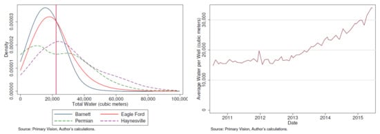
Figure 1.
Water Use in Hydraulic Fracturing.
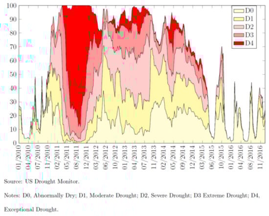
Figure 2.
Percentage Area of Texas in Drought by Severity.
High-frequency regional drought measures are provided by the United States Drought Monitor, which is produced collaboratively by the National Oceanic and Atmospheric Administration (NOAA), the U.S. Department of Agriculture (USDA), and the National Drought Mitigation Center (NDMC) at the University of Nebraska–Lincoln. The U.S. Drought Monitor provides a weekly measure of drought intensity by county according to five distinct drought intensity categories. The drought categories are abnormally dry (D0), moderate drought (D1), severe drought (D2), extreme drought (D3), and exceptional drought (D4). The weekly drought measure reports the percent of each county classified in each drought category. The drought status of a county is determined by five indicators: Palmer drought severity index, NOAA Climate Prediction Center’s soil moisture model, the United States Geological Survey weekly streamflow data, the standardized precipitation index model data, and NOAA objective blends of drought indicators.
Figure 2 plots the area of Texas in each drought category as a percent of the total area in the state over the sample period. The figure shows that both the severity of drought and the area in drought increased sharply beginning in late 2010. The drought severity peaked in the summer of 2011, and the most severe drought conditions abated by the end of 2012. However, a majority of Texas remained in some level of drought until 2015, with significant portions of the state in exceptional drought during that period.
The spatial variation of the Texas drought is illustrated in Appendix Figure A1, Figure A2 and Figure A3, which plot the drought severity in Texas. Prior to 2011 (Appendix Figure A1), there was no exceptional drought in Texas. At the peak of the drought (Appendix Figure A2), nearly the entire state was in extreme drought. By 2012 (Appendix Figure A3), exceptional drought remained in many counties. This spatial variation in drought data is a key component of our identification strategy.
In our sample, about 64% of observations are in the no drought category. Of the 46% of observations that fall within a drought condition, 13.3% are in category D4, exceptional drought. The average daily temperature in the sample was 19 °C. Our humidity measure, dew point temperature, measures the temperature at which water vapor condenses out of the air. The difference between dew point temperature and air temperature measures relative humidity (a large difference means very humid; a small difference means less so); during the sample period, the weather across Texas was somewhat humid.
3. Theory and Empirical Models
A stylized economic model motivated our empirical work, in which an oil producer completes wells, W, using inputs of capital, K, and labor, L. The three capital inputs for well completion are water, proppant, and chemicals, . Oil, O, is the output of the well completion process and is a function of the completion inputs, O = W(K, L). This simple model takes geological conditions as constant, which means that oil production depends solely on inputs into the well completion process. The producer chooses inputs to optimize oil revenue minus costs of completion,
where P is the price of oil and C(K, L) is the input cost function.
If we assume that the operator spends a fixed price for labor and capital inputs, the profit function becomes
where , and are wages, the costs of water inputs, proppant, and chemicals, respectively. This model shows that the profit-maximizing energy producer responds to an increase in water costs by lowering water input, thereby decreasing production. If we assume that second-order cross-derivatives of capital and labor inputs are zero, this can be shown by the partial derivative,
where , and are the second-order derivatives of the oil production function with respect to labor, chemicals, and proppant, respectively, which are all assumed to be negative from concavity in the production function. The denominator, det:H is the determinate of the Hessian matrix of the model, which is positive from the second-order sufficient condition for a maximum. The derivative is taken at the optimal values for all choice variables.
Given the results of the theory model, the key query for this paper is whether this reduction in water use is economically meaningful. That is, can we measure a reduction in water use and production during drought periods? We used several empirical models to estimate the effect of drought on unconventional energy production by examining whether operators cut back on the number of wells drilled or the water intensity of wells drilled in drought areas. The models shared a common identification strategy. We used exogenous variation in drought conditions to identify the effect of water scarcity on hydraulic fracturing activity. In the short run, technology is fixed, and producers can only respond to drought-induced input scarcity by some combination of decreasing input usage and/or increasing input spending. We estimated several reduced form regressions to understand the producer response to increased water scarcity. The drought variables provided the net effect of water scarcity on water prices accounting for producer responses. The reduced form parameters of interest were identified using cross-sectional and intertemporal variation in drought intensity across the counties in Texas, which was driven by exogenous weather shocks.
We used a panel data model, where the unit of observation is the county-week, to examine whether there were fewer wells drilled in counties during exceptional drought. We modeled the total number of wells drilled in county i at time t as follows,
where is the count of wells drilled. The controls, , include the real West Texas Intermediate (WTI) price, which affects drilling decisions [8], and county and month-of-sample fixed effects to control for county-level variation in geological conditions and trends over time in drilling, respectively. We used three different measures of drought conditions in county i at time t, . First, we used drought intensity during week i, to capture the contemporaneous drought conditions. Next, we used the average drought intensity in the twelve months preceding date t, to capture the drought conditions when operators were likely sourcing water. The relationship between these two drought measures and well counts is plotted in Figure 3. Finally, we used drought spell, or number of consecutive weeks of exceptional drought in county i at time t, to capture the effect of longer droughts. There is significant variation in drought spell; the average duration of an exceptional drought was about 20 weeks, though exceptional drought lasted over 140 weeks in some counties.
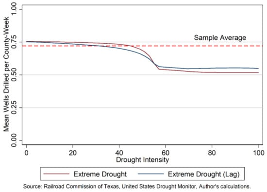
Figure 3.
Well Counts and Drought.
Next, we examined the effect of drought on well-level water use in well i, , using direct and indirect measures of well-level water use. Operator-reported water use data were used to directly measure water use, and the perforated zone length was used to indirectly measure water use. In the water use models, the unit of observation is the well, and the exogenous variation in weather conditions identifies the effect of drought on water intensity. The total amount of water used in well i,
where is a measure of the water used in well i. The drought measures and controls used in Equation (1) were used with one addition: the operator fixed effect. The operator fixed effect controls for time-invariant operator characteristics that impact water use choices. The drought measure for well i, , captured the drought conditions on the date that well i was completed (lag drought intensity and drought length (weeks)).
Given that gas and oil production is a function of the hydraulic fracturing inputs, we next investigated whether drought, at the time of the well completion, had an impact on production. The only mechanism through which drought could impact a well’s production is if the operator used less water because of water scarcity. The operator could lower water use by reducing the perforated zone or by simply using less water. The effect of drought at the time of completion on subsequent production from well i is modeled as,
where is the total (allocated) oil and gas production in first six months from well i that was drilled at time t. Importantly, the drought conditions measures for well i, , reflect drought conditions during well i’s completion. This model uses the same set of controls, , as the model presented in Equation (2): operator, county, month-of-sample fixed effects, and the WTI price.
4. Results
We begin by estimating the causal effect of exceptional drought on the number of wells drilled in a county using the panel data regression model specified in Equation (1). The results for two separate regressions, each with a different drought measure, are presented in Table 2. The first column reports the effect of lag exceptional drought intensity (measured in terms of percent of county in drought, from 0 to 100) on well counts in a given week. The lag drought intensity is the average drought intensity in a county during the previous three months. The second column reports the effect of exceptional drought length, in weeks, on well counts. For each specification, the county-level clustered standard errors are reported.
Table 2.
Drought and Drilling Regression Results.
Across specifications, we found a negative, statistically significant effect of exceptional drought in a county on the number of wells drilled in that county. In the first specification, where the lag exceptional drought measure was used, we found that exceptional drought covering 50% of a county would reduce the number of wells drilled in a week by 0.29. The estimated effect of drought length on well counts was similar; a year-long exceptional drought in a county would reduce the number of wells drilled in that county by 0.32. These declines were economically meaningful. In the Eagle Ford Shale, drilling reductions of this magnitude would represent about a 13% decline in the total number of wells drilled in a week. Taken together, these results confirm a fundamental result of the theory model; when a key input to hydraulic fracturing is extremely scarce in a given area, operators will complete relatively fewer wells in that area.
Next, we present the results from Equation (2), which estimates the causal effect of exceptional drought on well-level water use, as shown in Table 3. The estimated effect of drought on our direct measure of water use, total water per well, is reported in columns 1 and 2. Using the two different drought measures, lag drought intensity and drought spell, during the well completion, we found a negative, statistically significant relationship between drought and well-level water use. Wells drilled in a county that is 50% covered by exceptional drought would see a decline in water use per well of about 17%, and wells drilled in a county experiencing a year-long exceptional drought would reduce water use by 18%. The effect of exceptional drought on the indirect measure of water use, perforated zone length, is reported in columns 3 and 4. Again, there is a negative, statistically significant relationship between the two drought measures and this indirect measure of well-level water use. The magnitude of the effect of exceptional drought on perforated zone length (1–4%) is smaller in magnitude than the effect of exceptional drought on total water use. These regressions, which control for operator and county-level characteristics, demonstrate that operators completing wells in exceptional drought conditions directly respond to drought by adjusting the amount of water used per well and by reducing the perforated zone of the well.
Table 3.
Drought and Water Use Regression Results.
These results suggest that oil producers respond to exceptional drought conditions by both drilling fewer wells in drought areas and by completing wells with less water in drought areas. Exceptional drought causes reductions in both the total amount of water used in wells and the length of the perforated zone of the well. We estimated the empirical model presented in Equation (3) to determine whether these differences in the characteristics of wells completed in exceptional drought areas had a measurable effect on production from those wells. In other words, we investigated whether the drought-induced reduction in an input of hydraulic fracturing (water) caused a decline in the outputs of hydraulic fracturing (oil and natural gas). The results of the regressions for oil and natural gas wells are presented in Table 4. The results for the oil well model are presented in columns 1 and 2, and the results for the natural gas model are presented in columns 3 and 4. For both oil and natural gas wells, exceptional drought at the time of well completion had a statistically significant, negative effect on production during the first six months. The magnitude of the effect was similar for oil and gas wells using both drought measures: wells completed in a year-long exceptional drought, or in a county 50% covered in exceptional drought, produced about 12% less oil and gas.
Table 4.
Drought and Production Regression Results.
It is important to note that these results only applied to production during the first six months. Given that these wells were drilled fairly recently, and production can continue for years, we cannot estimate the impact of drought on long-term or cumulative production. Oil and gas production typically falls by 65–80% over the first twelve months, though production can continue for many years [9].
While these results suggest that wells completed during exceptional drought use less water during completion and produce less oil and gas relative to a counterfactual well completed in the same location in non-drought conditions, it is not clear that these effects are permanent. Operators could return after drought conditions subside and recomplete the wells, which would involve stopping production and hydraulically fracturing the well again to stimulate additional production. We conclude by investigating whether wells completed in drought conditions are recompleted at higher rates than wells completed in non-drought conditions. Recompletions are modeled as,
where is an indicator that well i is recompleted at some point in the future; are drought conditions during first completion of well I; and are the controls used in previous regressions, which include the real price of oil at time of completion and fixed effects for operator, county, and the month-of-sample of the original completion. As in the previous regressions, exogenous variation in the location and time of drought is used to identify the causal effect of exceptional drought conditions during completion on subsequent recompletion.
The results of the recompletion regressions are presented in Table 5. Neither the lagged exceptional drought nor the exceptional drought length at time of completion had a measurable effect on recompletions. As with production, it is important to note that these regressions estimated the short-run effect of drought on recompletions. The sample period covers wells recompleted between 2011 and 2017, so this regression would not capture recompletions occurring outside of the sample period. If, for example, drought at the time of well completion causes recompletions to rise five years later, our regressions would not capture this lagged effect.
Table 5.
Drought and Recompletion Regression Results.
5. Conclusions
Beginning in 2011, a prolonged heatwave and severe drought covered Texas. During this period hydraulic fracturing drastically increased drilling in shale basins throughout the state, requiring massive water inputs. We found that energy firms facing scarcity of a key input in the hydraulic fracturing process, changed their completion behavior in two key ways. First, we used a fixed effects model to show that operators completed fewer wells in counties experiencing exceptional drought, and these effects were pronounced for prolonged drought spells. Second, we found that operators working in drought areas reduced the amount of water used in each well. These operators also completed wells with shorter perforated zones, which means these wells required less water to fracture hydraulically. The reduction in the amount of water used to hydraulically fracture wells is the mechanism through which exceptional drought conditions during well completion reduced oil and natural gas production. Using well-level oil and natural gas production data, we found that exceptional drought during completion had a modest effect on oil and gas production. Though these wells appeared to extract less oil and gas than wells drilled in non-drought conditions, there was no evidence that these wells are recompleted at a higher rate.
These results have important implications for regulators, who have typically been concerned with the effect of water use in hydraulic fracturing on drought [10], though this research demonstrates that the important causal effect runs in the opposite direction, namely, drought has a measurable effect on hydraulic fracturing operations. The Railroad Commission of Texas, which is the state’s oil and gas regulator, is required by statute to, “prevent waste of the state’s natural resources”. Efficient extraction of oil and gas is in the interest of the state, which benefits from the economic activity, employment, and tax revenue generated by energy production. Allowing unconventional wells to be drilled and completed during periods of exceptional drought does not lead to efficient extraction of oil and natural gas. While the effect of drought oil and natural gas production may be relatively small for a given well, the aggregate impact on production from all wells completed during drought conditions is much larger. Between 2011 and 2015, 12% of wells were completed during drought conditions. This research demonstrates that these wells recovered less oil and gas than would have been recovered using wells drilled during non-drought conditions.
Author Contributions
Reid Stevens and Gregory Torell consulted experts, analyzed the data, and wrote the paper.
Conflicts of Interest
The authors declare no conflict of interest.
Appendix A. Drought in Texas
Drought Monitor data describe the area of Texas, by county, in each drought category over the sample period. There is substantial variation in drought conditions over time and across counties from 2010 through 2015. The drought severity did not increase until late 2010, and most of the state was in non-drought conditions as late as September 2010 (Figure A1). The drought severity peaked during the summer of 2011. During the peak period, almost all of Texas was in the most severe drought category (Figure A2). While the most severe drought conditions abated in the next year (Figure A3), a majority of Texas remained in some level of drought until 2015.
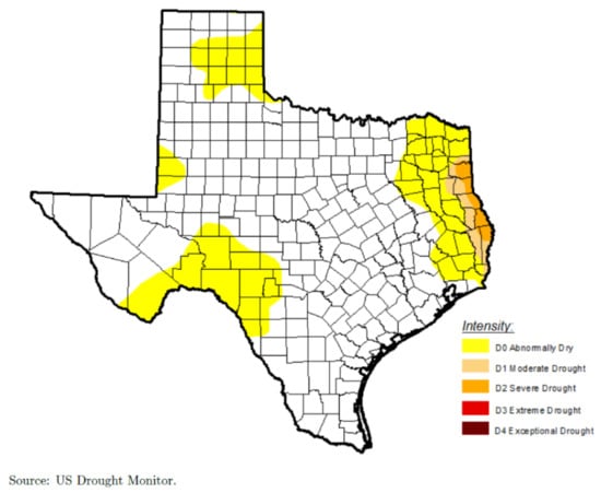
Figure A1.
Drought in Texas: 28 September 2010.
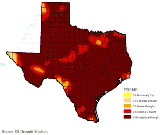
Figure A2.
Drought in Texas: 27 September 2011.
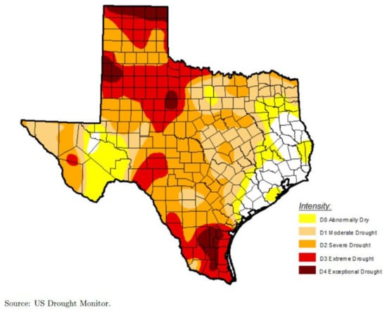
Figure A3.
Drought in Texas: 25 September 2012.
References
- Nicot, J.P.; Scanlon, B.R.; Reedy, R.C.; Costley, R.A. Source and Fate of Hydraulic Fracturing Water in the Barnett Shale: A Historical Perspective. Environ. Sci. Technol. 2014, 48, 2464–2471. [Google Scholar] [CrossRef] [PubMed]
- EIA. Trends in US Oil and Natural Gas Upstream Costs; United States Energy Information Administration: Washington, DC, USA, 2016. [Google Scholar]
- Shauk, Z. Drillers Looking at Cutting Need for Lots of Water. San Antonio Express. 19 September 2012. Available online: https://www.mysanantonio.com/business/article/Drillers-looking-at-cutting-need-for-lots-of-water-3878703.php (accessed on 4 April 2018).
- Covert, T. Experiential and social learning in firms: The case of hydraulic fracturing in the Bakken Shale. SSRN Electron. J. 2015. [Google Scholar] [CrossRef]
- Driver, A.; Wade, T. Fracking Without Freshwater at a West Texas Oilfield. Reuters. 21 November 2013. Available online: https://www.reuters.com/article/us-apache-water/fracking-without-freshwater-at-a-west-texas-oilfield-idUSBRE9AK08Z20131121 (accessed on 4 April 2018).
- Cook, M.; Webber, M. Food, Fracking, and Freshwater: The Potential for Markets and Cross-Sectoral Investments to Enable Water Conservation. Water 2016, 8, 45. [Google Scholar] [CrossRef]
- Kondash, A.; Vengosh, A. Water Footprint of Hydraulic Fracturing. Environ. Sci. Technol. Lett. 2015, 2, 276–280. [Google Scholar] [CrossRef]
- Anderson, S.T.; Kellogg, R.; Salant, S.W. Hotelling under Pressure; Working Paper 20280; National Bureau of Economic Research: Boston, MA, USA, 2014.
- Allen, W.; Lacewell, R.; Zinn, M. Water Value and Environmental Implications of Hydraulic Fracturing: Eagle-Ford Shale; Technical Report; Texas Water Resources Institute: College Station, TX, USA, 2014. [Google Scholar]
- EPA. Hydraulic Fracturing for Oil and Gas: Impacts from the Hydraulic Fracturing Water Cycle on Drinking Water Resources in the United States; United States Environmental Protection Agency: Washington, DC, USA, 2016. [Google Scholar]
© 2018 by the authors. Licensee MDPI, Basel, Switzerland. This article is an open access article distributed under the terms and conditions of the Creative Commons Attribution (CC BY) license (http://creativecommons.org/licenses/by/4.0/).