Article

Quantifying the State of the Art of Electric Powertrains in Battery Electric Vehicles: Comprehensive Analysis of the Two-Speed Transmission and 800 V Technology of the Porsche Taycan

Institute of Automotive Technology, Department of Mobility Systems Engineering, TUM School of Engineering & Design, Technical University of Munich, Boltzmannstr. 15, 85748 Garching, Germany
*
Author to whom correspondence should be addressed.
World Electr. Veh. J. 2025, 16(6), 296; https://doi.org/10.3390/wevj16060296
Submission received: 15 April 2025 / Revised: 14 May 2025 / Accepted: 20 May 2025 / Published: 27 May 2025

Abstract

:
In the automotive industry, battery electric vehicles (BEVs) represent the future of individual mobility. To establish a long-term market presence, innovative vehicle and powertrain concepts are essential, and therefore, identifying the most promising concepts is crucial to determine where to focus research and development further. Academia plays a significant role in this identification process; however, researchers often face restricted access to data from the industry, and identifying different technological approaches is often connected to significant costs. We present a comprehensive study of the Porsche Taycan Performance Battery Plus, which integrates two technological advancements: the first series-production implementation of a two-speed transmission in an electric vehicle allowing for high acceleration while reaching high top speeds and a 800 V battery system architecture providing more efficient charging capabilities. This study details vehicle dynamics, electric powertrain efficiencies, their impact on vehicle level, and the two technological advancements. This work aims to provide researchers access to vehicle dynamometer and real-world data from one of the most advanced and innovative battery electric sports cars. This allows for further analysis of cutting-edge technologies that have yet to reach the mass market. In addition to providing researchers with this study’s results, all data utilized in this study will be made available as open-access, enabling individual use of test data for parameter identification and the development of simulation models.

1. Introduction

The automotive industry has recently faced one of its biggest challenges, driven by global climate targets shifting towards electro-mobility [1]. The European Union (EU) mandates a significant reduction in fleet emissions for original equipment manufacturers (OEMs). To avoid penalties, they must reduce CO 2 emissions by 15% by 2025 and by 37.5 % by 2030 compared to 2021 [2]. As a result, manufacturers are increasingly focusing on BEVs, which are characterized by zero local emissions and high energy efficiency [3]. Accordingly, the registration of electric vehicles is increasing globally [4]. In Germany, the market share of BEVs reached 18.4 % in 2023, which is an increase of 11.4 % compared to the previous year [5].
Despite this trend toward electro-mobility, customers remain cautious regarding BEVs, being concerned about range limitations, accessibility of charging infrastructure, aging of battery packs, and the higher initial costs compared to conventional vehicles [6,7]. In a recent study, the most important customer-related features were identified, and the highest-ranked features were the electric range, the charging time, and energy consumption [8]. According to [9], global automotive companies plan to invest about USD 1.2 trillion in electro-mobility and battery technology. OEMs search for an optimal solution regarding electric vehicle technology, aiming to remain competitive or reach a technological advantage in this rising market [10].
Besides the concerns, BEVs provide many advantages, e.g., the reduction in required gears. Reducing the number of gears, and therefore the number of components, reduces the control complexity, the transmission mass, and thus the vehicle’s energy consumption. Most of the current BEV generation is equipped with a single-speed transmission, where their gear ratio is a compromise between acceleration from low vehicle speeds and a high top speed [11]. This compromise presents a challenge for sports car manufacturers, especially. Whereas most manufacturers currently rely on hybrid vehicles with electric machines supporting the combustion engine, Rimac installed a wheel-individual powered powertrain with four electric machines to avoid multi-speed transmission in their 2022 Nevera model [12]. The 2024 Mercedes-Benz G580 also has an individual powertrain for every wheel. Still, in addition to the electric machine at every wheel, a two-speed transmission provides a separate gear ratio for off-road scenarios [13]. Porsche, however, introduced a two-speed transmission solution for their first electric sports car, raising the question of whether a two-speed transmission and its increase in complexity can be beneficial for energy consumption or helps mainly to avoid the compromise of choosing a certain gear ratio [14]. The two-speed transmission of the Porsche Taycan will be explained in detail in Section 5.1. Also, whether a two-speed transmission optimizes efficiency depends on its gear shift timing strategy. Dynamic gear shift strategies focus on vehicle performance, whereas energy-efficient strategies optimize the powertrain’s efficiency [15].
InnoShiftIng GmbH [16] developed a multi-speed transmission specifically for electric vehicles in collaboration with the Technical University of Darmstadt, claiming to enable energy savings of 5% to 10% compared to a single-speed gearbox. A key component of this innovation is the redesigned actuator, which accelerates gear shifts by a factor of 10 to 20 [16]. Additionally, a combination of dog clutch and differential angle sensor ensures a more efficient power transfer, reliable synchronization, improved comfort, and reduced wear during shifting. Nevertheless, this technology is expected to reach production status in 2028 [16]. Laitinen et al. [17] analyzed the potential improvement in the energy efficiency of an electric vehicle (Nissan Leaf) equipped with single-speed and two-speed transmissions. Based on simulations, efficiency was evaluated across multiple driving cycles and in different scenarios. The study concluded that a two-speed transmission enhances the efficiency of an electric vehicle. Further potential could be achieved if the machine–inverter combination is specifically optimized for the two-speed transmission. However, the impact of the additional mass of a two-speed transmission compared to a single-speed transmission is not considered nor mentioned in this study.
Another technological advancement of the Porsche Taycan is its 800 V battery system, which will be explained in Section 5.2. The share of electric vehicles utilizing 800 V architectures is increasing compared to standard 400 V systems [18]. Whereas it was initially introduced in the premium segment, this technology is expected to expand into the mass market in the coming years [18]. However, even higher voltage architectures face challenges, as compatible components are not yet available in sufficient quantities or at competitive prices. Additionally, enhanced insulation is required, increasing both complexity and costs [11]. Nevertheless, Tesla plans to develop the Semi Truck, which is scheduled to be produced in 2025, based on a 1000 V architecture, aiming to reduce charging times [19].
Besides the industry, academia is also working on the current state-of-the-art electric vehicle and component concepts. Unfortunately, their access to data and test objects is limited [20]. However, some studies were conducted on the component level, and fewer studies on the vehicle level. Studies on the component level [21,22] focused on single components or the interaction between the components of the electric powertrain, whereas [23,24,25] were more focused on the vehicle level or the impact of components on the vehicle level. The largest study, the Advanced Vehicle Testing and Evaluation study [26], was conducted as a collaborative work led by the National Energy Technology Laboratory in America. Within this study, 30 BEVs were tested between 2011 and 2018, underlining the effort to conduct a study to this extent. While most of the tested vehicles were no longer state-of-the-art when the study was published, comprehensive studies on single vehicles provide detailed data on current state-of-the-art vehicles [27,28]. Within these studies, multiple objectives on a Volkswagen ID.3 Pro Performance (2020) and a Tesla Model 3 SR (2020) were observed, analyzing their behavior and control strategies as well as their component characteristics and their impact on vehicle level.

1.1. Contributions

This work presents a comprehensive analysis of the vehicle under study, a Porsche Taycan Performance Battery Plus from 2022, with a detailed analysis of the two-speed transmission and the 800 V battery system on the vehicle level as a subsequent step to [27,28] with advanced vehicle characteristics. Within this advanced analysis, we focus on the following aspects of this vehicle and its components:
  • Aerodynamic impact on driving dynamics.
    The vehicle under study includes active aerodynamic components that affect the driving resistance in respective driving situations and are controlled by the vehicle and driver inputs.
  • Electric powertrain efficiency with two gears.
    The transmission’s two gears provide two different efficiency maps of the power unit, including the inverter, the electric machine, and the transmission. This requires a gear shift heuristic with a strategy that is affected by selectable driving modes.
  • Range across driving modes and ambient conditions.
    The electric range of the vehicle under study and its energy consumption are investigated in various conditions and different driving modes. Official test cycles and real-world driving scenarios are performed. To determine the influence of ambient temperature, the vehicle’s warm-up behavior and constant velocity characteristics are observed in a climate chamber.
  • Two-speed transmission and 800 V architecture.
    The technological advancements with the two-speed transmission and the 800 V battery system and their potential optimization in energy consumption are investigated. The two-speed transmission is compared to a single-speed transmission’s materials and components, followed by a powertrain efficiency analysis. The 800 V system’s impact on the charging and discharging processes is observed, and potential energy or time savings are discussed.

1.2. Layout

The structure of the study is illustrated in Figure 1. In Section 2, the vehicle dynamics are investigated with the description of the vehicle under test and the data acquisition methodology, the procedure for the coast-down tests considering the active aerodynamics, and the driving dynamics results. In Section 3, the electric powertrain is analyzed by explaining the efficiency analysis procedure and the operation strategy investigation, concluding in the gear shift timing heuristics and the power unit efficiency maps in both gears. Concatenating the previous two sections, in Section 4, we observe the vehicle concept results with the real-world and test cycle electric range and energy consumption in various driving and ambient conditions. With Section 5, the study investigates the technological advancements, the two-speed transmission, and the 800 V battery system. In Section 6, the main findings of this work are concluded and summarized.

2. Vehicle Dynamics Investigation

At the beginning of this section, we introduce the vehicle under study and explain the data acquisition. Following, the test procedure of the vehicle dynamics observation is described before the results are shown and discussed to officially available parameters.

2.1. Vehicle Under Study and Data Acquisition

The first edition of the Porsche Taycan was introduced in 2019 as the company’s first fully electric vehicle. Porsche provided different specifications like the base model with a rear-wheel drive (RWD) [29], more advanced models with all-wheel drive (AWD) [30,31], and the top model with maximum power [32]. In addition to the powertrain topology, the vehicle comes with two battery pack options: a base model with a gross battery capacity of 79.2 kWh and a performance plus version containing a gross battery capacity of 93.4 kWh [33]. Also, the vehicle is available in various body styles, including a sedan, a station wagon (Sport Turismo) [34], and an off-road station wagon (Cross Turismo) [35]. Since generation II, a high-performance version (GT) has been introduced in 2024 [36]. All vehicles are based on the performance platform J1, which also represents the base of the Audi e-tron GT. This platform features a two-speed gearbox, a 800 V battery system technology, and an optimized battery housing for optimal installation space utilization.
The vehicle under study is the sedan base model version equipped with the bigger battery, officially referred to as Porsche Taycan Performance Battery Plus from April 2022. The power unit consists of an insulated-gate bipolar transistor (IGBT) inverter in combination with a permanent magnet synchronous motor (PSM) with a rated power of 280 kW reaching up to 350 kW of peak power in launch control (LC) mode, achieving an acceleration of 5.4 s from standstill to 100 km/h. The top speed is electronically limited to 230 km/h [37]. According to the Certificate of Conformity (CoC), the vehicle has a range of 484 km [38]. The complete vehicle specifications are summarized in Table A1 in Appendix A. The vehicle was acquired from an official Porsche dealership to ensure production status. The vehicle mass was measured to 2204 kg using FLP wheel-load scales in combination with a DFW-K series terminal (DINI ARGEO S.r.l., Modena, Italy). This presents a deviation of less than 1% compared to the 2205 kg specified by the manufacturer in the CoC. With the measurement equipment and the driver, the test mass was measured to 2307 kg.
In the vehicle under study, multiple active aerodynamic features are applied: First, at the vehicle’s front, active radiator shutters are individually controlled for the left and right-hand side by the respective electronic control unit (ECU). Closed shutters reduce the air resistance and, therefore, improve the efficiency and electric range of the vehicle. In contrast, open shutters increase the air stream to the radiators and thus improve the cooling [39]. At the rear of the vehicle, an active rear spoiler is controlled to either provide less aerodynamic drag for a higher electric range or to increase downforce for improved vehicle dynamics at higher speeds. The rear spoiler changes between four levels, increasing the so-called angle of attack with increasing vehicle speeds to maintain a stable driving condition [39]. Last is the ride height adjustment. Also, depending on the vehicle’s velocity, the chassis level is lowered with increasing velocity to decrease frontal area and thus decrease air resistance [40]. In contrast to the rear spoiler levels, the chassis level can be changed by the driver in the Porsche Communication Management, analogously like the suspension level. The manufacturer provides four different levels. Lift lifts the vehicle 20 mm in reference to Normal to prevent bottoming out (e.g., on steep inclines). Lowered is 10 mm lower than Normal, whereas Low decreases the chassis level by 22 mm, achieving the lowest frontal area, and thus air resistance [40].
In addition to the active aerodynamic components, the manufacturer provides three driving modes: Normal, where the vehicle focuses on comfort, Sport, which uses a stiffer suspension setup, selects a more aggressive motor torque control, and lowers the vehicle slightly to reach the optimal performance, and Range, which optimizes the energy consumption to reach optimal electric range contrary to Sport mode. To optimize the energy consumption, the vehicle decreases the top speed to 140 km/h and operates exclusively in second gear, except when full throttle is applied, eventually indicating a hazardous situation. As mentioned before, the chassis level is set to Low, and air conditioning (AC) and headlights are reduced. When starting the vehicle, it is set to Normal mode regardless of the prior selected mode, indicating its primary driving mode. According to EU Regulation 2017/1151 [41] and the Global Technical Regulation (GTR) 15 [42], this is the driving mode for official test procedures (i.e., Worldwide Harmonized Light Vehicles Test Procedure (WLTP)).
The measurement setup consists of a data-logging tool developed by Merkle et al. [43]. The tool collects the vehicle’s internal communication data between the ECUs based on querying their states via Unified Diagnostics Service (UDS) accessed by the onboard diagnostics (OBD)-II standardized port. Using a commercial diagnostic tool, the relevant message identifiers (IDs) have been observed and decoded to assign the actual physical value to the controller area network (CAN) communication signals. This method allows for measurements such as dynamometer tests and real-world driving scenarios on test tracks or public roads [44]. The logger sends requests of the desired signals to the vehicle and with a splitter cable connected to a VN1610 (Vector Informatik GmbH, Stuttgart, Germany), the responses are sent to a laptop and saved. The relevant IDs for this study with their signal addresses, properties, and their conversion factors to physical meaning are concatenated in Table A2 in Appendix B.

2.2. Vehicle Coast-Down Procedure and Driving Resistance Determination

In preparation for the coast-down tests, the active aerodynamics of the vehicle under study must be considered. According to [41,45,46], the setup for official test procedures requires the primary driving mode and, thus, the primary behavior of the aerodynamics. Since Normal and Range modes are investigated in the following sections, both are identified in the coast-down tests.
To analyze the aerodynamic parts, we recorded their behavior during real-world driving scenarios and specific test conditions. The rear spoiler level is solely based on the vehicle speed and regardless of the current driving mode, where hysteresis is applied to avoid oscillations. The active radiator shutters regulating the air stream to AC, water, and brake cooling are controlled more complexly. Since they remain closed during a Worldwide Harmonized Light Vehicles Test Cycle (WLTC), which is the driving cycle of the WLTP, we ensure the shutters remain closed during our coast-down tests to reach comparable results. The chassis level is controlled by the vehicle speed and the selected driving mode. This must be considered during the coast-down tests, delivering different coast-down curves and, thus, road load coefficients (RLCs).
The tests were performed on the test track of the University of the Bundeswehr in Neubiberg. Since the test track is only 1.6 km long, the coast-down was divided into multiple vehicle speed segments, which are shown in Table 1.
In addition to the speed segments, the following aspects are considered for Normal mode: The top speed of 95 km/h for the Medium chassis level results from the heuristic to switch to the Lowered level above. The Low level is reached at 198 km/h, and thus the Lowered level is used until the maximum speed of 160 km/h.
The coast-down segments were performed four times to smooth surface roughness and in both directions to eliminate inclination influences. The eight runs were concatenated into an average curve and smoothed by moving average filtering [47,48], resulting in one coast-down curve for every chassis level. The vehicle was prepared to operating condition, and all requirements in [45] regarding temperature and wind velocity were fulfilled.
To provide a coast-down curve for the Normal driving mode, the curves for Lowered from 160 km/h to 65 km/h and for Medium from 65 km/h to standstill are merged, since 65 km/h is the hysteresis point where the chassis level changes. The Range mode is the Low curve starting from 140 km/h considering the top speed in this driving mode. Note that the coast-downs are only recorded until 15 km/h since road surface influence dominates the measurement results according to [49].
For the measured coast-down curves, the RLCs are calculated by deriving the vehicle speed and fitting the profile to the parameters as follows:
d v d t = a ( v ) = f 0 + f 1 · v + f 2 · v 2 m ,
where f 0 , f 1 , f 2 represent the RLCs and the total mass m = m test + m r = m test + 0.03 · ( m test + 25 kg ) is the sum of the test mass m test and a factor for rotating parts m r according to [45].
When the RLCs are available, applying
v i + 1 = v i + f 0 + f 1 · v i + f 2 · v i 2 m · Δ t
converts them into a vehicle speed profile, which is required to compare the coefficients of official test procedures to the experimentally determined coast-down curves.

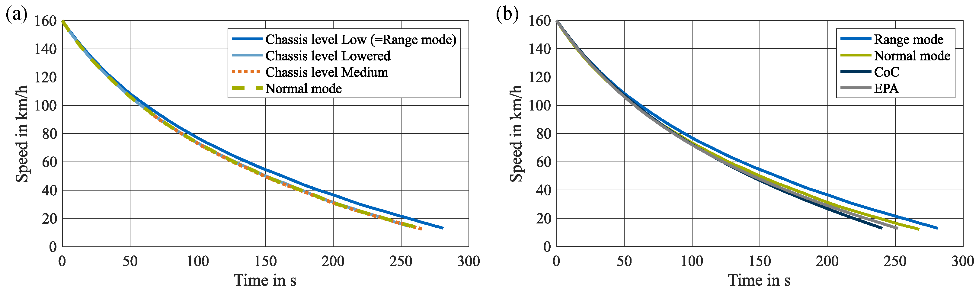
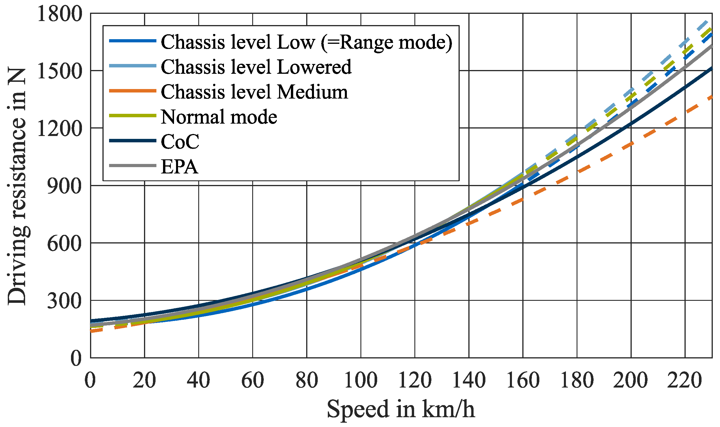
2.3. Driving Dynamics Results

All test procedures and their durations and distances, also of the following analyses, are summarized in Table A3 in Appendix C. The results of the performed coast-down tests are presented in Figure 2a, where the Lowered and Low chassis levels start at 160 km/h and the Medium level at 95 km/h. The Range mode equals the Low level, whereas the Normal mode combines the Lowered and Medium levels. Data have proven that both active radiator shutters remained closed during all coast-down segments.
It is shown that the Medium and Lowered levels do not present significant deviations from 95 km/h to 15 km/h, which is proven by a root mean square error (RMSE) of only 0.3 km/h, providing a meaningful result for the Normal mode. Considering the chassis level difference of 10 mm, the two levels do not show significant deviations, but optimizing the frontal area of the vehicle affects the air rather than the rolling resistance, which is dominant at lower speed levels. Air resistance has a squared impact on vehicle speed and, therefore, dominates at higher speeds.
The Low level, or the Range mode, is above the Normal mode curve and thus presents a slower decrease in vehicle speed and a longer coast-down time. This suits the aerodynamic optimization of lowering the vehicle to a further 12 mm, and with the higher vehicle speeds, the impact becomes significant.
In reference to the above-presented results, we generated the coast-down curves of official test results from their RLCs. In Figure 2b, our test results are compared to the official tests by the manufacturer in the CoC [38] and by the Environmental Protection Agency (EPA) [50]. Interestingly, both curves are below our results, indicating higher driving resistances.
It is important to consider the test masses of the respective test procedures. The vehicle under study reaches a total mass of m = 2377 kg, whereas the total mass in the CoC is m = 2360 kg, and of the EPA test, it is m = 2381 kg. To properly compare the results, identical total masses are required since higher masses result in higher inertia and, thus, in longer coast-downs. Therefore, it cannot be proven whether longer coast-downs are based on greater masses or better driving resistances.
Comparing vehicles with different masses, driving resistance forces are more suitable for analysis since they are independent of inertia. The RLCs derived from polynomial regression are concatenated in Table 2.
Although the chassis level mainly affects the air resistance and, thus, velocity-dependent coefficients, all coefficients deviate between the different test procedures. The coefficients for the Medium and Lowered levels showed significant differences, whereas their coast-down curves were nearly identical. This lies in the vehicle speed interval of the chassis level and, therefore, different data segments for the regression analysis. An analysis based on the RLCs is not recommended since these parameters are solely derived from mathematical regression.
Figure 3 shows the driving resistances of the different RLCs based on their respective test procedures. Note that the RLCs were derived from actual measurement points. The dotted lines indicate the extrapolated area.
In the valid area, the driving resistance curves show similar behavior, with the Range curve presenting the least resistance. The Medium level shows a lower slope in its extrapolated area compared to the curves, showing that the velocity-dependent rise in driving resistance is not properly covered until a vehicle speed of 95 km/h. In contrast, the CoC curve shows the highest resistance at lower speeds and the lowest at higher speeds, whereas the EPA curve shows a greater slope at higher speeds. The differences are caused by different test procedures or different vehicle speed intervals. However, since these curves are measured in the primary driving mode, the results must be compared with the Normal mode results, which shows reasonable comparison.
The Range curve shows lower resistances especially at higher speeds, proving the point of the optimized chassis level at higher speeds. However, with a lower chassis level, the suspension travel is reduced and thus ride comfort, and therefore, Normal mode focusing on comfort is operated at a higher chassis level [51].

3. Electric Powertrain Analysis

After the driving resistances of the vehicle under study are analyzed and discussed, the electric powertrain is investigated. The operating strategy of the power unit, consisting of an inverter, an electric machine, and a two-speed transmission, is investigated, i.e., its gear shift heuristic and the resulting two efficiency maps of the power unit.

3.1. Efficiency Analysis Procedure and Operation Strategy Investigation

To investigate the power unit’s behavior, we operate the vehicle on a vehicle dynamometer. The vehicle is set to a dynamometer, or Dyno mode, where advanced driver assistance systems (ADAS) are deactivated to prevent control interventions. In this section, we focus on the electric powertrain and not the overall vehicle, and thus, we neglect driving resistances and operate the vehicle dynamometer in velocity control mode. In this mode, the dynamometer is set to run at a specific vehicle speed. It remains at this speed regardless of the vehicle’s torque input, which allows to keep the vehicle at certain load points and adjust either torque or speed independently. To operate at defined accelerator pedal positions (APPs) and keep this position to reach reproducible results, an automatized brake and throttle control is implemented and installed.
First, we investigate the vehicle’s gear shift timing. The test specifications are as follows: Starting from a vehicle speed of 50 km/h, since the vehicle is in first gear in every driving mode, the APP is set and the vehicle velocity is increased by 1.8 km / h s to a final vehicle speed of 130 km/h, which is above the maximum speed in the first gear. The tests are performed in the state of charge (SOC) range of 30% to 70% and at the official reference temperature of 23 C . The test is also performed at a low-temperature level of 10 C , at low SOC levels, and different velocity ramps, but none of the parameters present any influence on the results.
Second, the efficiency maps of both gears are recorded. Test specifications are equal to the gear shift timing, but for this test, the vehicle is warmed up, so it is in operating condition. In contrast to the gear shift timing, specific load points are held constant and analyzed. These load points are kept for 30 s, besides load points at higher torques, which are only kept for 15 s since the torque is electronically reduced to restrict thermal load. In this test, the dynamometer is set to a specific vehicle speed, and the torque is set to different levels by adjusting the APP. To further control thermal load, the load points are alternated between high and low torque at constant vehicle speeds. The investigated torque levels are 5, 15, 30, 60, 90, 120, 150, 180, 210, 240, 270, 300 Nm and the available torque at 100% APP results in the full-load characteristic curve. The vehicle speed levels are 4, 8, 12, 16, 20, 24, 32, 40, 52, 64, 80, 96, 112, 128, 152, 176, 200, 224, and the top speed of 230 km/h. The lower areas of torque and speed are divided into smaller segments due to higher gradients in efficiency [27,28]. Normal and Range modes are applied to cover all available areas, and the procedure is adapted according to the findings of the gear shift analysis. Equation (3) describes the calculation of the power unit’s efficiency:
η Power unit = P Power unit , out P HV Battery , out ( P Aux LV , in + P Aux HV , in ) ,
where the electric power signals into the power unit are calculated by P electrical = U · I as the product of voltage and current [52], and the mechanical power out of the power unit is calculated by P mechanical = T · ω as the product of torque and angular velocity after the transmission [53]. Both auxiliaries, high-voltage (HV) and low-voltage (LV), are considered, and thus, differences in the driving modes are considered. The power into the auxiliaries can be summarized as the battery heating losses and direct current–direct current (DCDC) converter losses, where the voltage level is converted for the respective components.

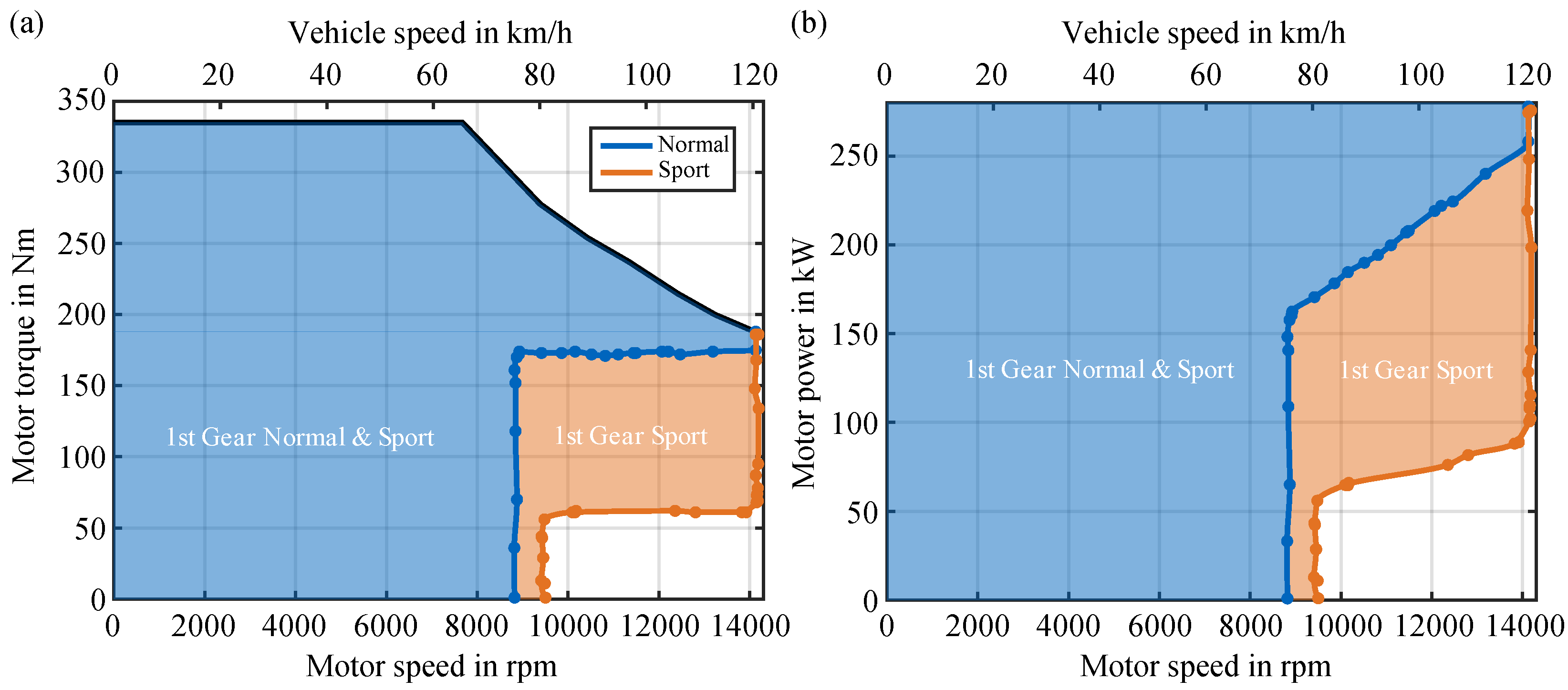
3.2. Gear Shift Timing Heuristic

First, the results are only shown for Normal and Sport mode since, in Range mode, the vehicle operates entirely in second gear. This only applies when the vehicle is in Dyno mode. When operated in real-world driving scenarios on public roads, the vehicle downshifts into first gear when the APP reaches a certain value, which might be based on providing maximum torque in potentially hazardous situations. For Normal and Sport mode, the downshift timing is at 54 km/h. However, applying the brake pedal downshifts is postponed until the brake pedal is released again.
Figure 4a shows the gear shift timing depending on the applied motor torque in Normal and Sport modes. In the unloaded scenario (i.e., APP equals 0%), the upshift is recorded at a motor speed of 8800 rpm, or a vehicle speed of 75 km/h for Normal mode, and in Sport mode, at a motor speed of 9500 rpm and a vehicle speed of 80 km/h.
The vertical lines at the presented motor speeds show that even with higher torques, the gear shift timing remains at these speeds. In both modes, this vertical curve changes at a certain torque into a horizontal curve; in Normal mode, this happens at 170 Nm, and in Sport mode, the torque is significantly lower at 62 Nm. This horizontal curve continues until a motor speed of 14,000 rpm, which equals a vehicle speed of 120 km/h. Considering this motor speed in second gear, the vehicle speed is at 230 km/h, equaling the electronically controlled top speed of the vehicle, which shows that 14,000 rpm is the electronically controlled maximum speed of the motor.
With these characteristics, the gear shift timing primarily depends on the machine’s power rather than its torque. In Figure 4b, the gear shift timings are compared to different motor power levels. In Normal mode, the gear shift remains at 75 km/h until a mechanical power of 150 kW. From this point, the power is linearly increased to 250 kW at the maximum motor speed of 14,000 rpm. In Sport mode, this linear dependency starts at a motor power of 50 kW. With a higher slope, the first gear is entirely utilized at a motor power of 100 kW.
The mechanical power of the vehicle is connected to the applied APP. That means that, similarly to the power, the gear shift timings are also linear and dependent on the APP. In Normal mode, this means that the upshift timing of 75 km/h is kept until an APP of 50%. Linearly rising up to 75% at 120 km/h, the first gear is fully utilized. In Sport mode, the upshift is until an APP of 25% at 80 km/h, also linearly increasing until 35%, fully utilizing first gear.
As shown, the gear shift timing depends on the APP, the driving mode, and the vehicle speed. These characteristics prove that with a certain power request, the gear shift is delayed until the base speed in the second gear is already reached. Thus, the maximum power is available, allowing for optimal performance. Otherwise, a potential reason for earlier gear shifts in Normal mode relies on comfort criteria reducing the noise, vibration, and harshness (NVH) load.

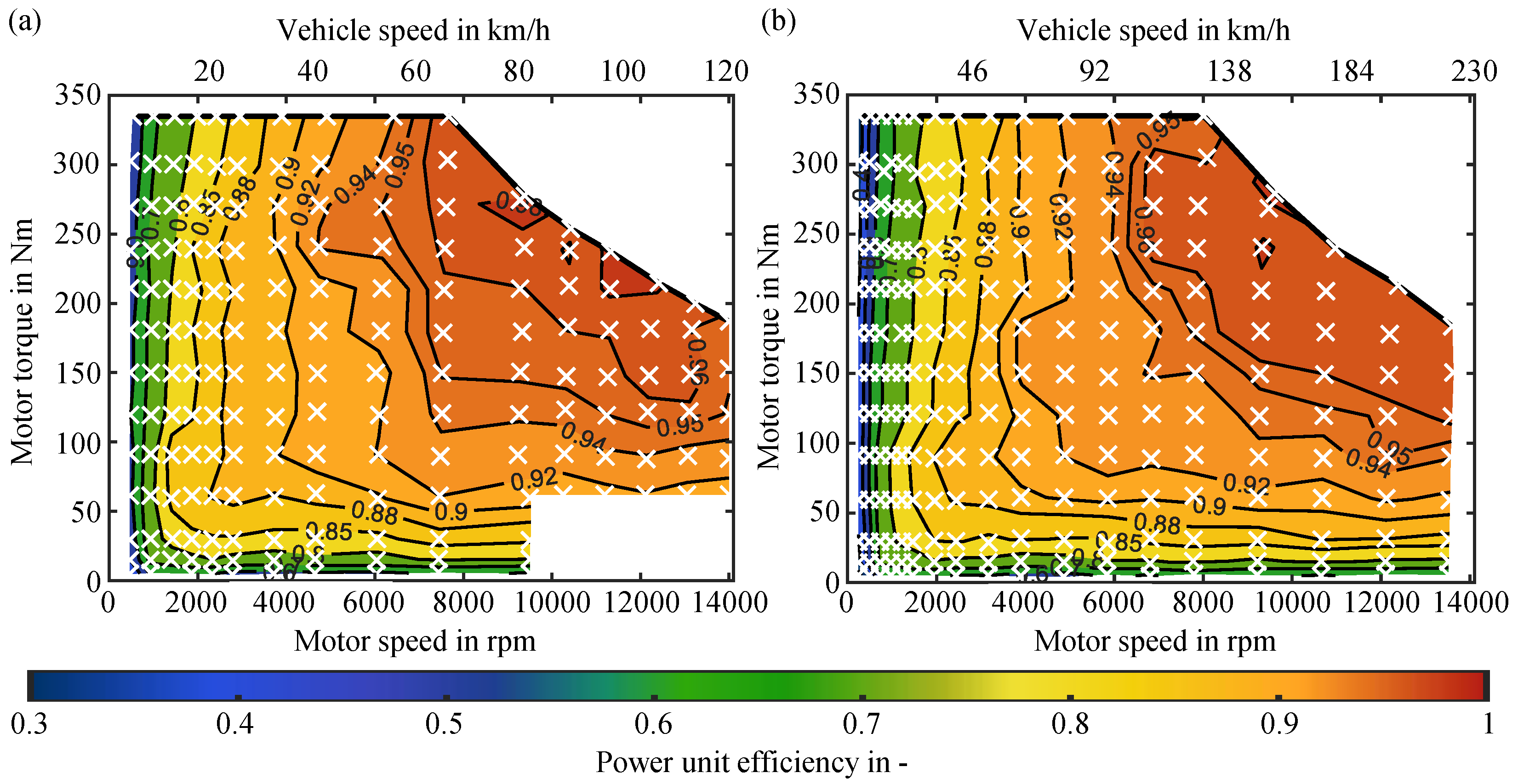
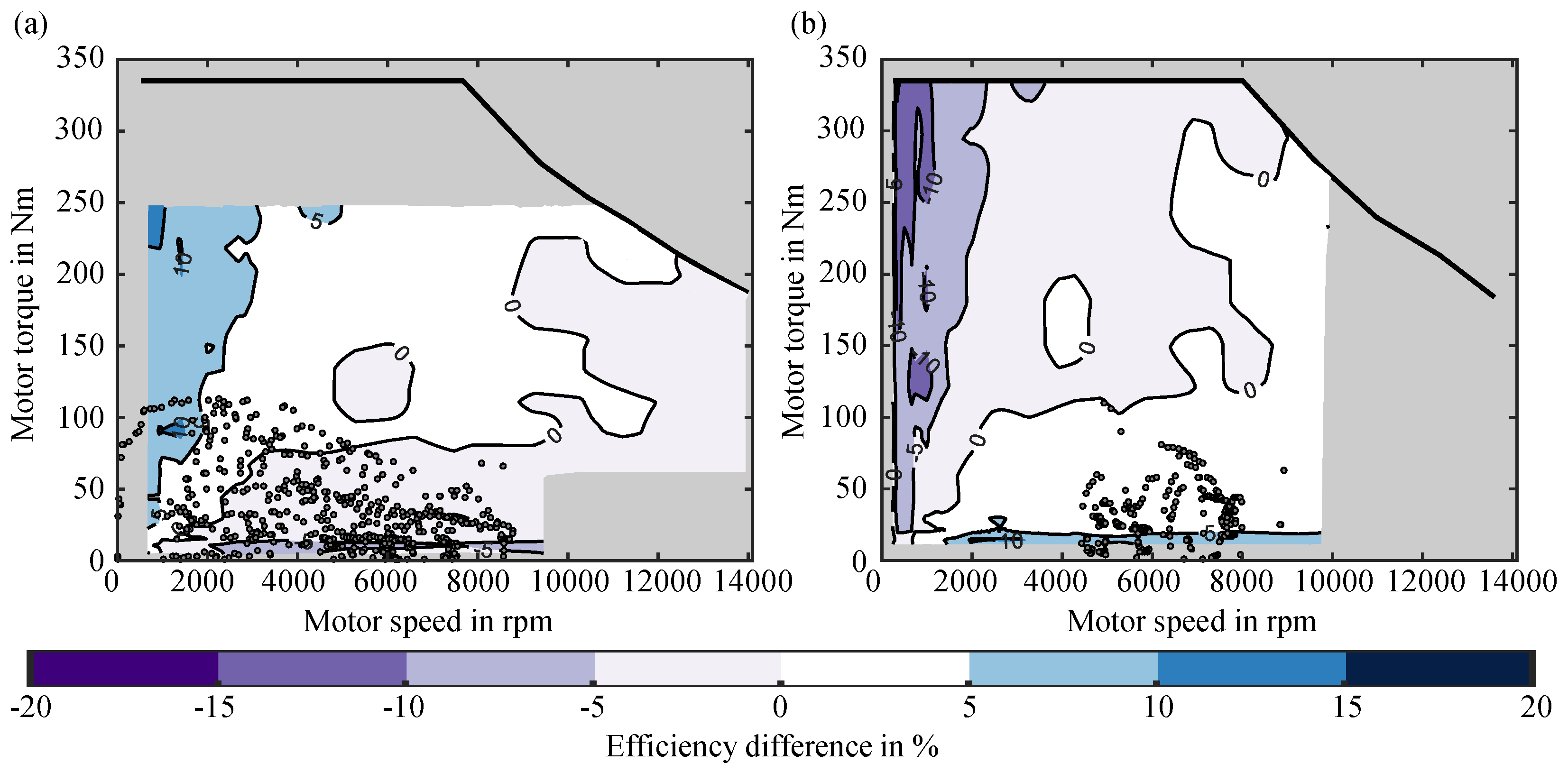
3.3. Power Unit Efficiency Results

The efficiency of the power unit is shown for both gears and compared. Since inverter and electric machine operate in analogy, the differences are mainly based on the two gears in the two-speed transmission. Thus, the differences are relatively small considering the high efficiencies in transmissions [54]. To cover the entire area in second gear, the lower speed areas were performed in Range mode. In second gear, a total of 223 load points were recorded and included in the efficiency map, whereas only 174 load points were recorded for the first gear, as shown in Figure 5a. The white area covers the part that cannot be driven in first gear, as shown in Figure 4. For the 32 load points above, Sport mode was activated.
According to the standard behavior of a PSM, the maximum efficiency is at high torques at rather higher speeds after the base speed [11,55]. From this area, the efficiency is reduced to low motor speed levels independent of motor torque and to lower motor torque levels independent of motor speed. The minimal efficiency of 39% is, therefore, at a low motor speed of 465 rpm and a motor torque of 5 Nm. The maximum efficiency of 97% is reached at a motor speed of 9375 rpm and a motor torque of 240 Nm. The rated torque of 335 Nm is available from a standstill until the base speed of 8000 rpm, as mentioned before. In contrast, in the CoC, the rated torque is given by 357 Nm, but this applies only in LC mode, which is only available in Sport mode. The torque then decreases degressively to a final value of 187 Nm, which is reached at the maximum speed of 14,000 rpm.
The efficiency map for the second gear is entirely covered. The efficiency map with all 223 load points is shown in Figure 5b. The full-load characteristics are the same according to rated torque, base speed, maximum speed, and torque at maximum speed.
The efficiency map shows a high gradient to low efficiencies for the second gear at lower motor speed levels. The minimum efficiency of 26%, reached at a motor speed of 240 rpm and a motor torque of 4 Nm, is smaller than the minimum value in first gear. Similar to the first gear, the area of maximum efficiency is at high torque and rather higher motor speed levels, with its maximum value of 98% reached at a motor speed of 9610 rpm and a motor torque of 279 Nm.
However, the difference between the two presented efficiency maps is shown in Figure 6. The grey area presents the parts of the efficiency maps that cannot be compared since at least one of the efficiency maps does not provide results. The reference map is the first gear, which means that positive values in the efficiency map describe areas where the first gear is more efficient than the second gear.
The efficiency maps of the power unit consider power losses of the inverter, electric machine, and transmission. Since the inverter and the electric machine work independently from the applied gear, the differences between the two gears represent the power loss differences in the transmission. Therefore, the differences in the efficiency map overlay are small, considering generally high efficiencies for electric vehicle transmissions [54]. The transmission design of the vehicle under study is described in detail in Section 5.1.

4. Vehicle Concept Observation

With the investigation of the driving resistances and the analysis of the electric powertrain, this section combines both results and observes the overall vehicle concept characteristics of the vehicle under study. First, we explain the performed test scenarios and their preparation to analyze the vehicle and its electric range in official driving cycles and real-world driving scenarios, which is most crucial to customers [8]. We investigate influencing factors on the range and assess the energy consumption during the warm-up phase and at constant vehicle speed levels at three different temperature levels.

4.1. Driving Resistance Simulation and Performance Validation

To assess the overall vehicle characteristics, the dynamometer is run in driving resistance simulation mode. This means the dynamometer no longer keeps a certain vehicle speed and changes the resistance according to the vehicle input. It provides a parametric resistance regardless of the input representing the vehicle on the road. In this mode, energy consumption and electric range tests are performed by considering the driving resistance that was observed during the presented coast-down tests. Since the dynamometer and public roads do not behave similarly, the dynamometer parameters are iteratively adapted until the vehicle shows the same coast-down characteristics. To validate this adaption process, a validation driving cycle is recorded on a public road. Then, the velocity profile is transferred to the dynamometer, and the results prove the parameter setup.
In the first test series, internationally standardized driving cycles (i.e., WLTP, Federal Test Procedure 75 (FTP-75), and Highway Fuel Economy Test (HWFET)) from Europe and the United States of America are performed. In addition, we apply real-world driving scenarios, including an Urban cycle with a total length of 8.1 km, an Interurban cycle of 20.1 km, and a Highway cycle of 35.2 km [27,28]. Following official test procedure standards [45,56], the electric range is measured by repeating the driving cycle until the vehicle can no longer follow the velocity profile, which is reached when the required velocity deviates from the tolerance of 2 km/h for 4 s. Thus, the test cycle is aborted. According to official test standards, the reference temperature of 23 ± 2 ° C is set for all test cycles. To ensure reproducible results, the vehicle is warmed up into operating condition and recharged, and an automatized brake and throttle control is applied, which fulfills the test procedures standards. Also, the cabin heating, ventilation, and air conditioning (HVAC) are deactivated in the driving cycle analysis. In addition, the infotainment system was switched off, but the headlights are turned on when the vehicle is ready to drive. To adequately calculate the energy consumption, the vehicle is recharged at a constant power of 22 kW. The charging efficiency η charge , 22 kW is calculated by
η charge , 22 kW = E Bat E AC = t 0 t end U Bat · I Bat d t E AC ,
where E Bat describes the energy into the battery and E AC the energy out of the charging station. The electric range and energy consumption for all cycles, including the American ones, are calculated according to the WLTP standard to reach comparability. The energy until the termination criterion E REESS is calculated by
E REESS = 1 3600 t 0 t end U ( t ) REESS · I ( t ) d t .
The electric range R WLTP equals the quotient of E REESS and the average energy consumption per cycle E C ¯ cycle , where the energy out of the battery per cycle E Bat , cycle divided by the distance during one cycle s cycle equals E C ¯ cycle [41].
In the second test series, we investigate the vehicle’s behavior at different temperature levels. First, instead of starting from operating condition, we record the warm-up of the vehicle under study at 7 and 35 ° C , which represents extreme climate conditions based on [57,58] and at the official reference temperature of 23 ° C [45]. After the vehicle is pre-conditioned overnight within the climate chamber, the measurement starts right after switching the vehicle on. We then proceed with the first cycle and continue as long as we achieve two following cycles with near-constant energy consumption and the vehicle in operating condition based on the respective ambient temperature. During the 7 and 35 ° C measurements, cabin heating is set to 22 ° C , and ventilation is set to Auto mode. After warm-up, we analyze the vehicle’s constant velocity energy consumption. In contrast to the first test series, we project this energy consumption to an electric range rather than driving the vehicle until it can no longer keep this velocity. The vehicle levels of 10, 30, 50, 70, 80, 100, 120, 130, 140, 160, 180, 200 km/h are kept for 3 min. These velocity levels are based on German speed limits. The velocity levels are driven in a pyramid profile; at first, the velocities are increased until the maximum level, and then afterward, they are decreased down to the lowest speed level. The final energy consumption is calculated based on the mean of the two measurements, except for the highest vehicle speed. For every 3 min measurement, the optimal phase of 150 s is considered for evaluation. For the vehicle speed of 70 km/h, there is one measurement in the first and one in the second gear based on the gear shift hysteresis for up and downshifts. In Range mode, the vehicle’s top speed is 140 km/h. Therefore, this is the top level of the test pyramid.
In both test series, the driving modes are considered. However, instead of considering Normal and Sport modes like in the previous section, we now consider Normal as the primary driving mode and Range mode. Sport mode mainly changes gear shift timing, the responsiveness of the electric machine, and the stiffness of the suspension, thus influencing driving cycle investigations less. In Range mode, however, we have a different chassis level, which provides a different set of driving resistances, different auxiliary behavior, and smoother electric machine control, effectively introducing two influential factors.

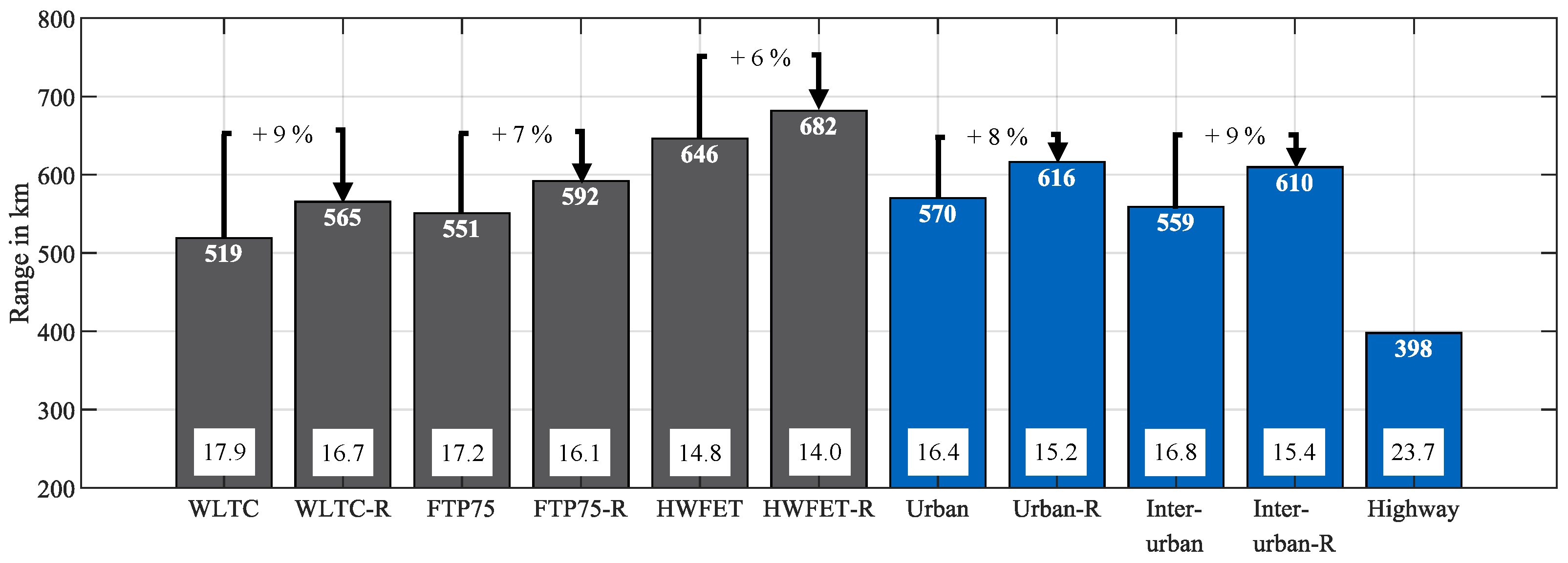
4.2. Real-World Range and Influencing Factors

The electric range is one of the most crucial, if not the most crucial, parameter in customers’ purchase decisions [8]. However, before analyzing the cycle ranges and energy consumption in the discharge direction, the charging process is observed. With a charging power of 22 kW, the charging efficiency of the vehicle under study is η charge , 22 kW = 88.73 % through a recharged energy capacity of 95.8 kWh from 0–100% SOC. In 2022, the Allgemeiner Deutscher Automobil-Club e.V. (ADAC) tested a Porsche Taycan 4S with the same battery capacity and cell chemistry with a charging power of 11 kW and measured the energy to E AC = 95.2 kWh from 0–100% SOC, equaling a charging efficiency of η charge , 22 kW = 89.26 % [59]. Smaller deviations can occur from charging power differences or from ambient temperatures, which are not specified by the ADAC.
Figure 7 presents test cycle results considering driving modes and chassis level. Note that in Range mode, the top speed is limited to 140 km/h, and the real-world driving Highway cycle includes vehicle speeds up to 159 km/h; this cycle has only been performed in Normal mode.
In the figure, the bars present the achieved electric range in the different test cycles given at the end of each bar. The numbers at the start of each bar present the energy consumption calculated based on the electric range, the covered distance, and the charging efficiency according to the previous equations. On the abscissa, the test cycles are presented, where the -R indicates the cycle was performed in Range mode. The grey bars show the official test cycles, and the blue bars show the real-world driving-based cycles [27,28].
The range results show, for the European reference cycle (WLTC), an electric range of 519.3 km. In comparison to this, the city cycles (FTP-75 and Urban) reach electric ranges of 550.8 km and 570.1 km, which equals an increase of 6% and 10%, respectively. The highest electric range of 646.3 km is achieved in the HWFET cycle, equaling an increase of 24%, and the lowest electric range of 397.8 km was achieved within the Highway cycle, equaling a decrease of 23%. Energy consumption is similar to the electric range. The WLTC has an energy consumption of 17.94 kWh 100 km . In contrast, the city cycles consume between 16.44 kWh 100 km and 17.19 kWh 100 km of energy. The lowest energy consumption of 14.82 kWh 100 km is reached at the HWFET and, analogously to the range, the highest consumption is 23.71 kWh 100 km , reached during the Highway cycle.
To validate these results, we want to compare them to the results given by the manufacturer in the CoC. Note that the RLCs given in the CoC indicate higher driving resistances, and thus, a lower range would be reasonable. Especially in the area of low vehicle speed, the driving resistances measured within this study are lower. With the WLTC mostly operating within this area, the differences of 19.8 % in energy consumption with a total of 21.5 kWh 100 km and 7.3 % in electric range with a total of 484 km compared to the data given in the CoC, the differences are reasonable according to the driving resistances. Interestingly, the deviations between electric range and energy consumption differ significantly. Although the energy consumption is based on the achieved electric range, the CoC does not provide information about the charging efficiency; the product of energy consumption and electric range equals an energy of 104.1 kWh. In contrast, this study’s consumed energy before reaching the termination criterion was only 93.2 kWh, which is confirmed by the ADAC measurement [59].
The Range mode results are next to the Normal mode results in the respective test cycles. The main difference between the two modes is the chassis level, which shows the greatest differences between Medium and Low levels (22 mm) until a velocity of 95 km/h or 65 km/h, respectively, when the vehicle decreases the chassis level to the Lowered level in Normal mode. The second major difference is the gear; as mentioned before, in Range mode, the vehicle is mostly driven in second gear, except at a standstill. This is related to the gear shift mechanism, where the multi-plate clutch is engaged in second gear, and thus, at a standstill, the vehicle switches back to first gear (see Section 5.1).
The optimization in the electric range is given above the respective bars, and through all cycles, the Range mode provides higher electric range results. As discussed before, the deviations in the range cannot directly be transferred to the energy consumption deviations since the energy consumption considers charging efficiency. In both modes, the achieved average vehicle speed is equal; only the vehicle speed at the termination criterion differs. The range results of the city cycles differ between 7.0 % and 8.1 %, presenting test cycles at rather low to medium vehicle speeds, restricting the influence of the RLC differences. The WLTC and Interurban cycles present cycles with higher dynamics and rather higher vehicle speeds, and thus, the driving resistances affect greater differences of 8.9 % and 9.1 %. Although the American HWFET cycle shows the highest average vehicle speed, it also shows the lowest dynamics. In this cycle, both driving modes mostly operate in second gear, and thus, it achieves the lowest difference in electric range with only 5.6 %.
The auxiliaries provide a near-constant power loss of P Aux = 500 W in Normal mode and 480 W in Range mode. Note that the rather small deviations between the two modes are based on the fact that the HVAC was turned off during the test cycles as specified in the official standards [45].
To identify and analyze the effect of the driving resistances and the driving modes separately, we perform an additional test series, where the vehicle is run for three WLTC cycles on the dynamometer with four different specifications: Figure 8 illustrates these four specifications. Indicated in the scheme of chassis level-driving mode on the abscissa, on the very left side, the Normal mode with its standard driving resistances is shown. Next to this, the RLCs for the Range mode but driven in the Normal mode are presented. The opposite is shown right next to that, where the RLCs of the Normal mode, or rather the combination of Medium and Lowered chassis levels, are operated in the Range mode, and on the far right side, the standard Range mode is illustrated, showing the RLCs of the Range mode operated in the Range mode. Note that the results do not match the results in Figure 8 since the measurement methods differ.
The electric range is calculated from the energy consumption during the three cycles, and based on the quotient of the net battery capacity and the recorded mean energy consumption, the projected electric range is calculated. As expected, the highest energy consumption and the lowest electric range are recorded in the standard Normal mode with the RLCs of this driving mode. Also, the lowest energy consumption and the highest electric range are achieved in Range mode with the RLCs of this driving mode. Based on the comparison in the shortened test procedure, the difference of 6.6 % is lower than the 8.9 % from before. More interestingly, we can see that the influence of road load coefficients or driving resistances affects the results more. Thus, the Low chassis level driven in Normal mode achieves a lower energy consumption and higher electric range than the chassis level in Normal mode operated in Range mode. In total, their difference is only 4 km. However, this is affected by the HVAC being switched off, which also influences the power losses in the two driving modes.

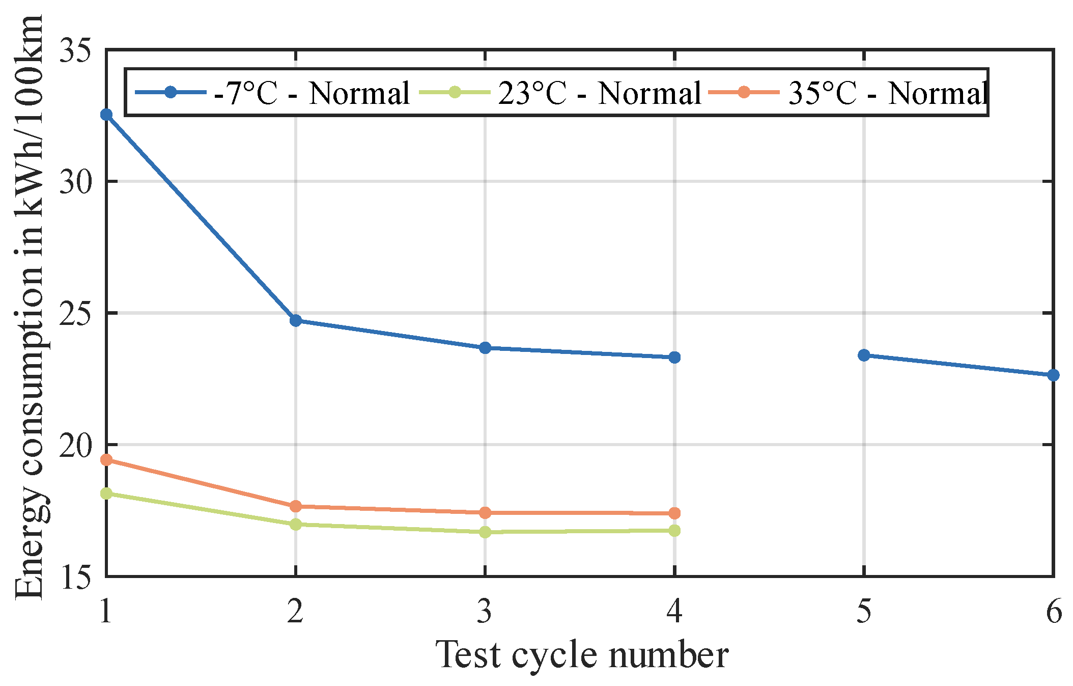
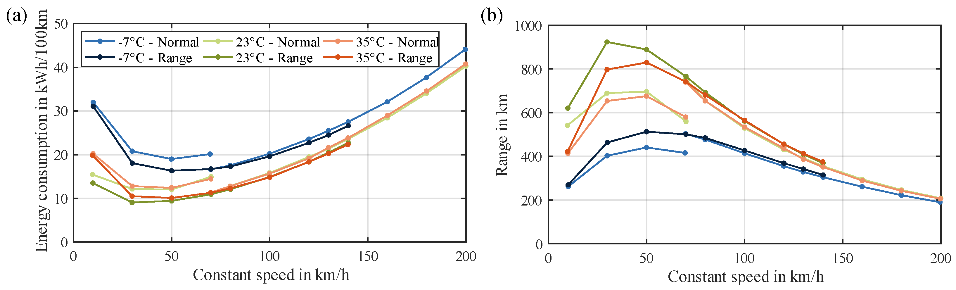
4.3. Warm-Up Behavior and Constant Velocity Range at Different Temperature Levels

In this final step of analyzing the electric range of the vehicle under study, we want to investigate the vehicle’s behavior based on different temperature levels. First, the vehicle’s warm-up behavior was observed. In Figure 9, this behavior is shown based on the three different ambient temperatures. As targeted, we stopped the measurement when the vehicle reached two following cycles with near-constant energy consumption. The test at 7 ° C yielded the biggest challenge since the warm-up took too long and the SOC dropped significantly, not allowing us to reach the operating condition and a near-constant behavior before recharging. Therefore, we had to recharge the vehicle and include a constant velocity phase to bring the vehicle into operating condition.
The blue graph shows the warm-up behavior of the vehicle at 7 ° C . The disconnection between the fourth and the fifth cycle indicates the recharging process and the constant velocity phase to reach operating conditions. At this temperature level, the energy consumption drops from 32.5 kWh 100 km in the first cycle to 24.7 kWh 100 km in the second cycle, yielding a decrease of 24%, which represents the biggest improvement of all temperature levels. This is explained by the HV heater, which boosts the battery temperature whilst consuming 4.3 kW on average ( 9.9 kW peak) from very low levels into acceptable temperature ranges, where the AC compressor takes over, reaching only 2.2 kW at peak, and the HV heater is switched off. Therefore, and through the increased battery and interior temperature from the second cycle, significantly less energy is required (AC compressor only requires 1.6 kW). Even when operating condition is reached in the sixth cycle, the energy consumption of 22.6 kWh 100 km is still 35.3 % higher than the energy consumption of 16.7 kWh 100 km in operating condition at 23 ° C , which is already reached in the third cycle.
The energy consumption at 23 ° C (standard temperature) appears to yield an optimal condition for the vehicle, whereas at 35 ° C , it the energy consumption reaches similar but slightly higher results with a near-constant difference of 4.2 %. The warmer temperature levels also show that the operating condition is reached after fewer cycles.
After the vehicle reached operating condition, the energy consumption for different constant velocity levels was investigated. Figure 10a shows the calculated energy consumption for the vehicle speed levels in the two driving modes at the three temperature levels, resulting in six curves. In Range mode, the results are connected in a continuous curve, in Normal mode, two separate curves are achieved considering the two gears applied according to the vehicle speed. These curves end or start at the vehicle speed of 70 km/h, available in both gears. Moreover, both modes show similar behavior for the three temperature levels, starting with high energy consumption at lower speeds, decreasing until a vehicle speed of 50 km/h, and then progressively increasing until the top speed.
Based on the temperature levels, the results for 7 ° C present the highest energy consumption throughout the entire vehicle speed range, whereas at higher speeds, the difference decreases, especially considering the relative deviation; the biggest deviation is at the lowest speed level of 10 km/h. In Range mode, the energy consumption of 31.1 kWh 100 km is even higher at this speed than compared to the maximum speed of 140 km/h, where the energy consumption reaches 26.7 kWh 100 km . The highest overall energy consumption is at the tested top speed of 200 km/h, where it reaches 44.1 kWh 100 km . Whereas the standard test temperature and the hot temperature test record nearly identical energy consumption with 40.3 kWh 100 km and 40.7 kWh 100 km , respectively, they reach their biggest deviation at 10 km/h, indicating a bigger impact of the auxiliary losses mainly caused by the HVAC, since operating condition is reached. Thus, the HV heater is switched off compared to Figure 9. Note that after the gear shift, the consumption between Normal and Range modes is nearly identical at all three temperature levels with increasing deviations with rising vehicle speed, showing the increasing influence of the driving resistance differences at higher vehicle speeds.
Figure 10b presents these energy consumption results analogously to the calculations in Figure 8 converted into projected electric ranges. The minimum electric range is reached, as before, at the highest vehicle speed at 7 ° C , where only 189.8 km are achieved. The highest electric range, however, at 30 km/h and at 23 ° C in Range mode, is 923.6 km, resulting in a difference of factor 4.9 . For the standard temperature level, the simulated WLTC range is achieved at a constant vehicle speed of 100 km/h with an electric range of 529.2 km in Normal mode and 561.5 km in Range mode.
The vehicle speed of 70 km/h, presenting the last measurement point of the first and the first point of the second gear, provides a direct comparison between the two gear ratios at this particular speed. In contrast to the Range mode, the same driving resistances apply here in second gear as in first gear. The biggest step between first and second gear is reached at the 23 ° C level, where the energy consumption of 15.0 kWh 100 km drops to 11.1 kWh 100 km in second gear, reaching a reduction of 26%. Note that this difference is potentially affected not only by the gear ratio but also by the measurement method, which does not allow for a mean value at this vehicle speed.

5. Technology Advancement Investigation

After the vehicle was analyzed at vehicle level on the chassis dynamometer, in this section, the technological advancements of the vehicle under study are described in more detail and compared to its predecessors. Since this is Porsche’s first model, we compare it against a previous vehicle model from the Volkswagen Group, whose insights may have potentially influenced the development and design decisions of this vehicle. The vehicle that provides the most detailed insights is the Volkswagen ID.3 [27].

5.1. Two-Speed Transmission Investigation

The first technological advancement is the two-speed transmission, which is the first such design to be applied in an electric sports car. It solves the compromise in a single-speed transmission, where either high wheel torques (independent from motor torque) are available at low vehicle speeds. Thus, better acceleration characteristics are achieved, or lower wheel torques are accepted to allow for higher vehicle top speeds. In this case, the first gear allows for optimized acceleration, and the second gear allows for higher vehicle top speeds and potentially optimized energy consumption, accepting higher transmission mass and more complexity through additional components and a shifting mechanism.
Its schematics are illustrated in Figure 11, with the numbers indicating the power flow through the components. The first shaft corresponds to the transmission input shaft, which is connected to the electric machine. The second shaft on the lower right corner features a coaxial shaft arrangement. The input shaft drives the inner shaft. The coaxial shafts are connected to the central shafts of the planetary gear set. A wet-running multi-plate clutch is integrated into the planetary gear set. The sun shaft is fixed or locked by the dog clutch and the freewheel, depending on the selected gear and driving direction. On the third shaft, the differential is located, and the output shaft leads to the wheels. The shift drum with ball ramp mechanism, the combination of dog clutch and freewheel, and the multi-plate clutch integrated into the planetary gear set form the shifting elements for gear changes.
The upshift sequence described is based on manually moving and interpreting the transmission components after its teardown. Therefore, it might differ from the presented gear shift behavior. The schematics and the parking lock function are based on [60,61]. It is electrically shifted by moving a shift drum with a ball ramp mechanism. The sun gear shaft is connected to the dog clutch and the freewheel. The rotational movement is transmitted to the ball ramp via a spur gear. Due to the ramp inclination, a shift fork is moved axially toward the central housing wall. This axial displacement activates the internally slotted disc spring. The shift mechanism is divided into four states:
The first state describes the parking lock function. The shift fork is in its end position relative to the left housing wall, so the sun shaft is fixed by the dog clutch. Furthermore, the inner spring element, the disc spring, is unloaded. The outer ring of the pre-loaded disc spring compresses the multi-plate clutch, blocking the planetary gear set. Due to the fixed sun shaft and the blocked planetary gear set, all transmission shafts are prevented from rotating.
The second state enables driving forward in first gear and backward as reverse gear. The ball ramp is rotated by a certain angle, causing the disc spring to be pressed internally. This eliminates the contact pressure on the multi-plate clutch, allowing the friction partners to exhibit a speed differential and, therefore, presents the favored position at a standstill. However, the sun gear remains fixed by the dog clutch.
In the third state, the ball ramp is rotated to push the sun shaft out of the dog clutch. Due to the freewheel, the sun shaft can only rotate in one direction. In the opposite direction, rotation is prevented by the freewheel. The multi-plate clutch remains disengaged. The exact function of this state cannot be clearly described, but it is suspected to represent a transitional phase between the two gears to avoid torque shocks during the gear change.
In the final state, the transmission is in second gear. Beyond a certain rotational angle, the inclination of the ball ramp decreases. The disc spring is no longer internally loaded, causing the plates of the clutch to be engaged. Since the sun shaft can still rotate in one direction, the planetary gear set and, consequently, the entire second shaft rotate at the same speed.

5.1.1. Materials and Components Comparison

With the transmission design and the gear shift mechanism explained, we mentioned additional components and complexity as a limiting or challenging factor of the two-speed transmission. Therefore, in this section, the additional components are compared, the resulting mass difference between a single-speed and a two-speed transmission is described, and the impact on the overall vehicle mass and, thus, energy consumption are analyzed through longitudinal dynamics simulations.
First, to investigate the impact of the transmission mass, the components of the two transmission designs with their different total masses are shown in Table 3. For the vehicle under study, the additional and more complex components have a total mass of 62 kg. In contrast, the single-speed transmission of the Volkswagen ID.3 only reaches a total mass of 24.51 kg, resulting in a mass difference of 37.49 kg. The impact of this difference is computed through longitudinal dynamics simulations, where the vehicle under study is implemented with its test mass of m test = 2307 kg and its vehicle specifications are given in Appendix A.
With the WLTC as speed profile, the simulation model is run with the actual test mass m two - speed = 2307 kg and then with a mass of m Porsche , sin gle - speed = m Porsche , two - speed Δ transmission = 2269.5 kg. The deviation in traction force is Δ F = 89.23 kN, which is small compared to the total traction force of F Porsche , two - speed = 6.93 MN in the WLTC for the original test mass model, resulting in a deviation of only 1.29 %. Transferring this deviation to the energy consumption, the energy consumption of 17.94 kWh 100 km is increased to 18.17 kWh 100 km and the electric range is reduced from 519.3 km to 512.6 km.
On the contrary, if the Volkswagen ID.3 with a test mass of m VW , sin gle - speed = 1937.5 kg [44] was equipped with a two-speed transmission, the mass would be increased to m VW , two - speed = m VW , sin gle - speed + Δ transmission = 1975 kg. The same simulation is performed for the Volkswagen ID.3 with the specifications given in [27]. Although the vehicle mass is significantly lower, the deviation in traction force is only 1.4 %, resulting in an electric range reduction from 415 km to 409.2 km.

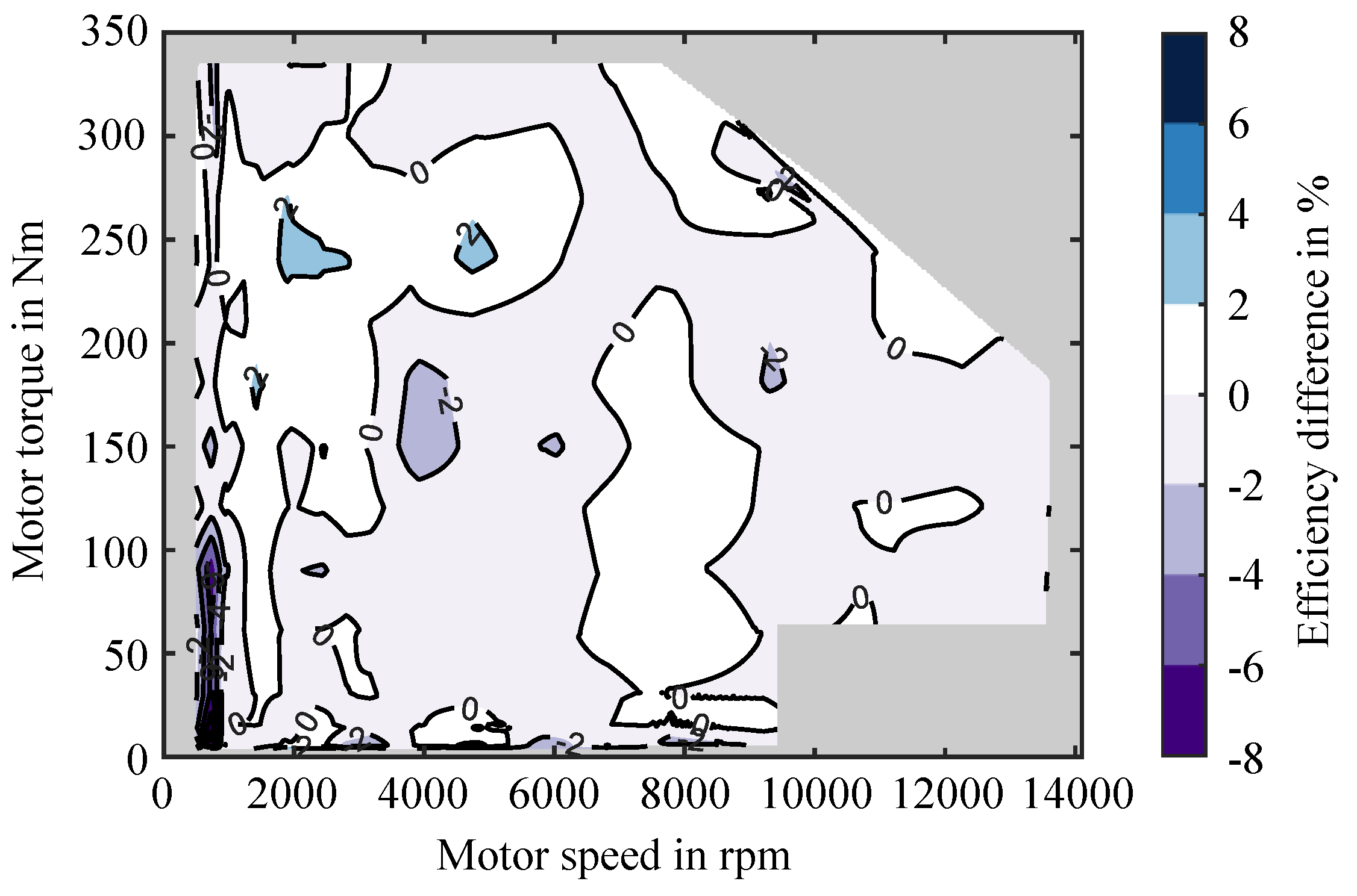
5.1.2. Influence on Power Unit Efficiency and Electric Range

Even though the mass differences between single-speed and two-speed transmissions proved neglectable, we now analyze the potential efficiency optimizations mentioned before, similarly to [17]. It was also mentioned that applying a single-speed transmission is a compromise and, therefore, would be set between the two chosen two-speed gears. To apply this idea, we use the Volkswagen’s gear ratio of i VW = 11.53 as the compromise, which is close to the average of the two Porsche gear ratio i ¯ Porsche = 11.86 . So, we shift the load points that were measured during one test cycle of the performed range tests in Section 4.2 from the first gear and the second gear of the vehicle under study into this compromise gear and observe its difference in efficiency. Note that we measured the efficiency in traction and, therefore, restricted the analysis to the propulsion load points. This prohibits any direct comparison to the analysis in the previous section. Considering a maximum motor speed of 14,000 rpm, the vehicle can reach all vehicle speeds of the presented test cycles. Since we cannot generate a new efficiency map according to this theoretical compromise gear, we use the second gear’s efficiency map from Section 3.3; first, because it is covered more extensively, and second, since it presents the parallel axis spurs gear set ratio with the planetary gear set not engaged, it is more comparable to a potential compromise gear set like applied in the ID.3.
Based on the load point shift, we investigate the difference in efficiency and, thus, the energy out of the battery required to follow the test cycles. For the load point shift from the first into the compromise gear, the motor speed is reduced, and motor torque is increased. Considering the investigated efficiency maps, below 150 Nm, the efficiency levels are nearly parallel to the abscissa, and below 5000 rpm, they are nearly parallel to the ordinate. Therefore, motor torque increases have a positive effect, and motor speed decreases have a negative effect on efficiency. Since both happen from the first gear to compromise gear, a potential optimization is load point-dependent.
To visualize this pattern, Figure 12a shows the area where the load shift into the compromise gear increases the efficiency indicated with negative values and a decrease in efficiency in positive values, in reference to the first gear, respectively. The values show the absolute difference in efficiency in percent. The figure also shows the load point during the WLTC test cycle.
The figure presents the areas of high torque and lower speeds with a negative impact on the gear ratio change. Still, most of the load points (during the WLTC) are within the purple area, where the efficiency is positively affected by the gear ratio change. Note that load points in the grey area are not considered. The final results for every test cycle are given in Table 4 on the left side. This table shows the differences in the energy out of the battery required to follow the speed profiles in the respective test cycles. The left side shows the required energy in kWh with the load points in the first gear, and the right side shows the load points shifted to the compromise gear ratio of 11.53 of the ID.3 [27] but applied to the efficiency map of the second gear. The percentual difference from the energy indicates the decrease in efficiency in accordance with the sign in Figure 12a, where a negative value indicates an optimization by changing the gear ratio.
Throughout every test cycle, the required energy is reduced when applying the speed profiles to the compromise gear. The percentual difference is independent of the absolute energy consumed during the test cycle. Note that the absolute energy is only for the first gear, and therefore, the Highway cycle requires less energy than the WLTC, for example, since the Highway cycle is mainly driven in second gear.
Analogously to the load point shift from the first into the compromise gear, all load points from the second gear are shifted to this compromise gear. However, here, a load shift leads to an increase in motor speed and a decrease in motor torque. Figure 12b shows the impact on the efficiency shifting from the second into the compromise gear. As before, in reference to the second gear, positive values describe an efficiency decrease, and negative ones an increase in efficiency.
Therefore, none of the load points from the WLTC lead to an increase in efficiency when shifting the gear ratio. This is also shown in Figure 5b, where the area from 5000 to 14,000 rpm below 150 Nm presents efficiency levels parallel to the abscissa, and since reducing the motor torque, the load points are shifted to worse efficiency levels. This is equivalent to the other test cycles. On the right side of Table 4, the results for the second to compromise gear shift are concatenated. Since the Urban cycle is completely driven in first gear, there are no results for this cycle. In contrast to the first-gear results, the positive differences indicate a reduction in efficiency. This is based on the torque reduction when changing to a higher gear ratio.
When both gear ratio changes are combined, concerning the results for the city cycles, including the FTP-75 ( Δ FTP = 0.36 %) and the Urban cycle ( Δ Urban = 0.68 %), a compromise gear would increase the efficiency. Meanwhile, an efficiency reduction compared to the two-speed transmission is observed for rising vehicle speeds. The WLTC reaches an efficiency difference of Δ WLTC = + 0.30 %, and the Interurban cycle a difference of Δ Interurban = + 1.15 %. The highway cycles, with the highest share driven in the second gear, reach the highest differences of Δ Highway = + 1.50 % and of Δ HWFET = + 3.11 %.
In conclusion, the results of the two-speed transmission analysis show that a two-speed transmission increases the powertrain mass. Still, considering the high overall vehicle mass, it is neglectable. Applying a second gear improves the efficiency, and for most test cycles, this means an optimization compared to a single-speed transmission with a compromise gear. In addition, two separate gear ratios provide better acceleration from lower vehicle speeds and allow for a higher vehicle top speed. In contrast, a two-speed transmission requires more components and is, therefore, more expensive and complex to control.

5.2. 800 V Architecture Analysis

After investigating the two-speed transmission as the first technological advancement compared to predecessors from the Volkswagen Group, the second technological advancement is analyzed: the 800 V high-voltage battery system. The voltage level of the battery system is defined by the series-connected cells. Whereas a 400 V system theoretically allows for a maximum charging power of 200 kW, considering a maximum current of 500 A, a 800 V system would allow for twice the charging power [62]. However, considering equal charging power, the current would be decreased [11]. Thus, conductor cross-sections and insulation could be decreased, which positively impacts the overall weight of the vehicle [63]. Additionally, the temperature increases proportionally to the square of the current [64]. Consequently, when comparing a 400 V to a 800 V voltage, assuming the same nominal power, only a quarter of the temperature increase from the ambient temperature is expected [64].
The 800 V system of the vehicle under study directly supplies the 800 V components, i.e., the inverter, the battery heater, and direct current–direct current (DCDC) converters, which convert the voltage level to 400 V supplying the HVAC, and to 12 V supplying the ECUs and the LV battery. Other Taycan versions also have 48 V systems installed, supplying Porsche’s dynamic chassis control system.
Analyzing the battery system’s technological advancement, discharging, and charging is interesting. For the charging scenario, as mentioned before, a higher voltage level allows higher nominal powers; what will be discussed is comparing the direct current(DC) charging processes of the vehicle under study against its predecessor, the Volkswagen ID.3, equipped with a 400 V system. The discharging scenario requires a more detailed observation of the battery system, and therefore, the power or rather energy losses are divided along the electric powertrain. Starting from the wheels, the Wheel-to-Distance (WtD) losses describe the driving resistance losses through the RLCs [27].
E WtD = 0 t P WtD d t = 0 t ( f 0 + f 1 · v + f 2 · v 2 ) · v d t .
The energy losses from the wheels to the inverter are described by the Inverter-to-Wheel (ItW) losses, which include the transmission, the electric machine, and the inverter, i.e., the power unit, plus mechanical braking. As mentioned before in Equation (3), the ItW losses are as follows:
E ItW = 0 t P HV Battery , out P WtD P Aux , in d t .
The auxiliaries build the third group of the energy losses, given by
E Aux = 0 t P Aux d t ,
including the losses into the direct current–direct current (DCDC) converter and to the battery heater, as stated before. The internal battery losses or, rather, ohmic losses, represent the final group, and are described as
E Ohm = 0 t I Bat , out n cell , par 2 R i · n cell d t .
The internal resistance of the cells was measured in a VC 3 4100 thermal camber (Vötsch Industrietechnik GmbH, Balingen-Frommern, Germany) with the cell connected to two parallel-connected channels of an MRS 6 V battery cycler (BaSyTec GmbH, Asselfingen, Germany). The resistance of R i = 1.243 m Ω was measured in reference conditions of 50% SOC, 20 ° C , 1 C, and a 10 s discharge pulse according to [27].

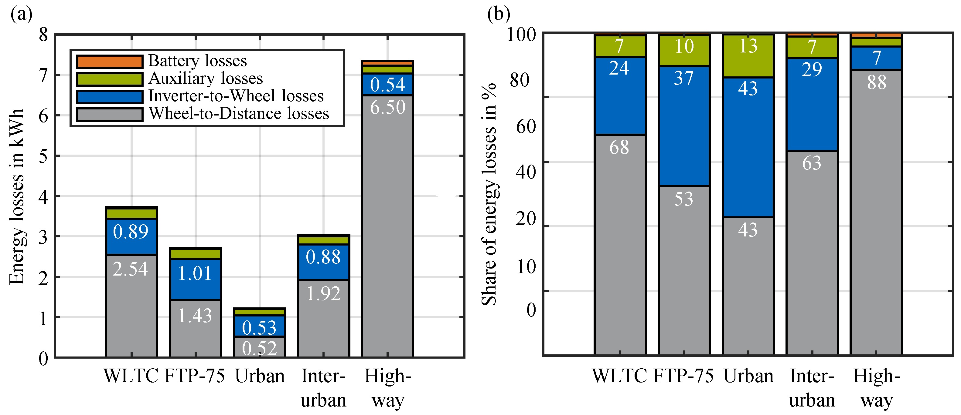
5.2.1. Efficiency Share Analysis

In this section, the energy losses are divided into the presented shares and investigated through driving cycles. This combines energy losses in different driving situations, such as traction, recuperation, and standstill. The energy share losses were calculated analogously to the reference study [27] and thus will be discussed, representing 800 V and 400 V systems. Table 5 shows the energy shares of the two compared vehicles in the described categories, with their absolute losses of the consumed energy during one cycle.
To illustrate this table, the total energy losses are shown in Figure 13a for the vehicle under study. The total energy losses depend on the speed profile characteristics and the duration of the respective test cycle. Regarding battery losses, the vehicle under study has lower energy losses across all cycles. This difference is based on the 800 V battery system and the associated current levels. In this system, lower currents are required for the same power output compared to the 400 V system model. As a result, the Porsche achieves lower battery losses, particularly at higher electrical power levels, and thus, higher currents. Therefore, the most significant differences between the two vehicles are observed during the Highway cycle.
In contrast, the auxiliary losses are higher in this study’s vehicle for all cycles except for the Highway cycle. The reason is the higher base load of the auxiliary components: whereas this vehicle requires a base load of nearly constant 500 W, the ID.3 uses only 300 W [27]. Consequently, this leads to a higher energy consumption for the Porsche. Note that during the Highway cycle, the Volkswagen requires increased power due to cooling peaks of up to 3.4 kW [27]. In comparison, the Porsche only requires 0.9 kW of cooling power during this cycle.
The ItW losses combine the electric powertrain and the mechanical braking losses. When comparing the powertrain efficiency, the Volkswagen achieves a 6.5 % to 7% higher efficiency than the Porsche in all test cycles except the Highway cycle. In this test cycle, the efficiency is 3.5 % higher. This almost fully transfers to the ItW losses; the Porsche reaches higher losses in all cycles, except for the Highway cycle; in this test, the Porsche even reaches a better result. This is based on the recuperation of the Porsche since it allows for higher electrical power to be fed into the battery system and, therefore, less mechanical braking. Thus, the dissipative energy losses are reduced.
The highest recuperation power was achieved during the Interurban cycle with 125.9 kW and the Highway cycle with 163.4 kW. With higher vehicle speeds, the mechanical power rises with the same negative motor torque applied to the wheels.
The final category, the WtD losses, depends on the driving resistance parameters and the vehicle speed, as given in Equation (6). As both vehicles perform the same speed profiles in the test cycles, the differences rely on driving resistances, including vehicle mass. Therefore, the Porsche reaches higher driving resistances at every speed level, thus reaching higher WtD losses.
Regarding the total losses, the Porsche consistently achieves higher losses than the ID.3 across all cycles, except for the Highway cycle. For the remaining cycles, the higher ItW and auxiliary losses of the Porsche lead to higher overall losses, which the optimized battery losses and recuperative braking savings cannot compensate for. To improve the comparison between the test cycles, in the parentheses of Table 5, the normalized results of both vehicles are provided.
Similarly to the absolute test results, Figure 13b illustrates the relative losses, allowing for a better analysis of the energy share losses. Also, Figure 15 in [27] shows the corresponding figure improving comparability. The battery share losses are small compared to the other energy share losses and smaller than the ID.3’s battery losses in all cycles, especially in cycles with high power demands. Whereas the percentual difference in the Urban cycle is only 0.67 %, the difference in the Highway cycle sums up to 2.35 %.
The auxiliary loss differences are based on their maxima and cycle durations. Consequently, city cycles present the highest shares, while highway cycles show the lowest shares. Comparing the two vehicles, the proportional auxiliary losses of the Porsche are higher across all cycles except for the Highway cycle. Since the proportional losses are normalized relative to the cycles, deviations for all cycles (excluding the Highway cycle) remain within a similar range between 2% and 2.72 % of difference. For the Highway cycle, Porsche’s auxiliary losses differ by 0.17 % from those of Volkswagen, which is based on Volkswagen’s additional cooling power requirements. As a result of the combination of powertrain and mechanical braking losses, urban driving cycles show the highest shares in ItW losses, while highway cycles have the lowest shares. Furthermore, the Porsche reaches higher proportional losses in all cycles except for the Highway cycle compared to the Volkswagen.
The WtD losses, or rather the driving resistance losses of the Porsche, are lower regarding their energy shares across all cycles, except for the Highway cycle. These proportionally higher WtD losses in the Highway cycle are based on Porsche’s comparably lower energy losses in the other categories. In the remaining cycles, Porsche’s total losses are correspondingly higher, which reduces the proportional WtD losses. Consequently, this study’s vehicle shows lower WtD shares compared to ID.3.

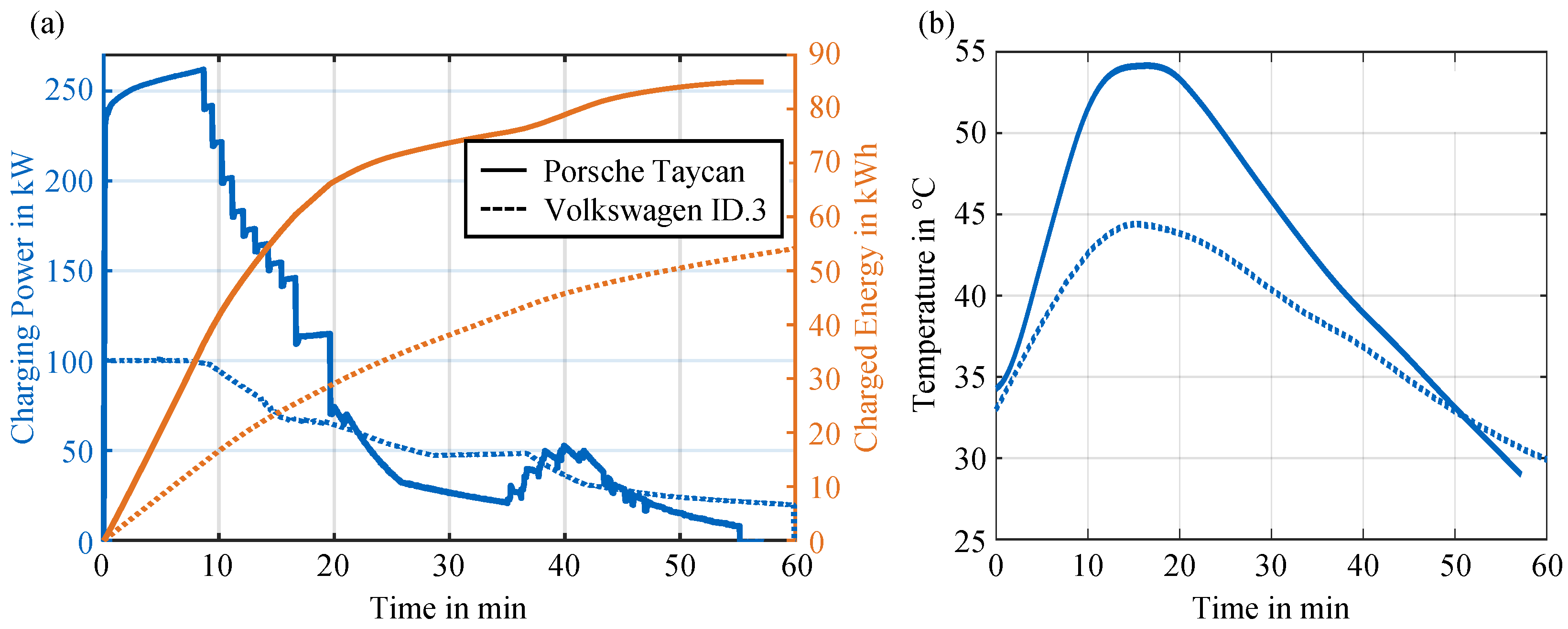
5.2.2. Fast Charging Optimization

With the discharge behavior of the 800 V system having been investigated, we now compare the differences in charging scenarios. The charging measurements were conducted at a 400 V DC charging station for the ID.3 measurement [27] and an 800 V DC charging station for the Porsche to prevent any converter losses. The charging process started pre-conditioned at a battery system temperature of 35 ° C for the Porsche and 34 ° C for the VW. In both vehicles, measurements were taken from 5% to 100% SOC. Figure 14a shows the charging power with the corresponding energy charged into the battery.
In the first 20 min, the Porsche consistently achieves a higher charging power than the Volkswagen. During this phase, the Porsche charges 66.6 kWh, which is about a factor of 2.3 higher than the 29.1 kWh charged to the Volkswagen. After this period, the charging power of the Porsche decreases to that of the ID.3. The complete charging process takes 57.22 min for the Porsche at an average charging power of 89.11 kW, compared to the ID.3’s charging duration of 59.87 min and an average power of 54.21 kW.
The Porsche’s higher charging power is connected to the larger energy storage capacity of the traction battery. With higher capacity, the C-rates decrease for the same currents. In addition, the 800 V technology allows for lower currents at the same power, which doubles the advantage and generates less heat during charging.
The highest charging power for both vehicles is achieved within the first 9 min: 262.2 kW for the Porsche (slightly lower than the manufacturer’s given value of 270 kW) and 100.2 kW for the ID.3. Note that the Porsche’s charging power ramps up during this period, whereas the Volkswagen maintains a constant charging power. Generally, battery voltage increases with rising SOC. Therefore, the ID.3 regulates the current downward as the battery voltage increases to maintain a constant charging power. In contrast, the Porsche maintains a constant current of 335 A, causing the charging power to rise slightly in the first 9 min, which might indicate a current limit. Furthermore, after this 9 min period, the charging power of the Porsche decreases in steps, indicating that the control algorithm aims to provide the maximum possible charging power. In contrast, the ID.3’s charging power decreases linearly after 9 min, suggesting a less complex charging performance control. A potential reason for the power decrease in both vehicles after 9 min is a reduction in power based on the increased battery system temperature.
For the Porsche, the battery temperature’s initial increase is nearly constant, as shown in Figure 14b. After 8 min, this slope decreases, and after 14 min, it is maintained at a temperature of 54 ° C for 4 min. This temperature curve correlates with the charging power. After 9 min, the charging control reduces the power to ensure that the battery system temperature does not exceed the 54 ° C . A similar temperature profile is recorded for the Volkswagen. Here, the temperature increases constantly for 8 min and reaches its maximum of 44 ° C after 14 min. Accordingly, the battery system temperature potentially presents the limiting factor for the charging performance control. Unlike the Porsche, the Volkswagen does not maintain the maximum temperature level, which also indicates a less performant charging process. Note that besides the power control and thus the temperature control, the charging strategy in the Porsche allows for higher absolute battery system temperatures, which might present as something learned from former vehicle models.
According to Equation (9), the ohmic losses depend on cell resistances and currents. Since the charging power in the Porsche is higher for the first 17 min, the currents are accordingly high. Overall, the ohmic energy losses in the Porsche are E Ohm , Porsche = 3.14 kWh, which is higher than the E Ohm , VW = 2.16 kWh for the ID.3. However, considering the energy into the battery of E charge , Porsche = 84.99 kWh compared to the E charge , VW = 54.09 kWh, the share of the ohmic losses in the Porsche 3.7 % is actually lower than the Volkswagen’s 4.0 %.

6. Summary and Conclusions

This work presents a comprehensive analysis of the Porsche Taycan on the vehicle level with all technological advancements considered. From the active aerodynamic parts influencing the vehicle dynamics and driving resistances to the two-speed transmission influencing the electric powertrain’s efficiency and driving modes impacting gear shift strategy and energy consumption or electric range. The 800 V architecture is investigated and compared to one of the Volkswagen group’s predecessors [27]. The major discoveries of this study can be summarized as follows:
  • Aerodynamic impact on driving dynamics.
    The vehicle under study is equipped with active aerodynamic components that influence the vehicle dynamics and, thus, the driving resistances of the vehicle under study. With the chassis level as the main contributor to driving resistance changes, the chassis levels are essential in describing the current operating mode.
  • Electric powertrain efficiency with two gears.
    Analyzing the vehicle’s electric powertrain characteristics, its gear shift strategy was identified with the APP, the vehicle speed, and the driving mode as the main influencing factors of the heuristic. This results in two respective efficiency maps of the power unit consisting of the inverter, electric machine, and the two-speed transmission. It is observed that the efficiencies vary by small margins based on the transmission characteristics.
  • Range across driving modes and ambient conditions.
    The combination of driving resistances in the respective driving modes and the electric powertrain efficiency in two gears results in the vehicle concept behavior. The influence of these characteristics is shown through official and real-world test cycles. The Normal mode is compared to the Range mode, which achieves significantly greater electric ranges. The climate chamber tests prove that electric vehicles struggle in cold conditions and that vehicles work optimally in official test conditions.
  • Two-speed transmission and 800 V architecture.
    The technological advancements of this vehicle prove optimization potentials, with the two-speed transmission neglectably increasing the vehicle’s overall mass and, therefore, not influencing the electric range. The 800 V system results show improved charging capabilities and lower internal battery losses during discharging. Considering higher cost and complexity, the advancements improve the vehicle’s overall efficiency characteristics.

Author Contributions

N.R.: Conceptualization, Methodology, Investigation, Resources, Writing—Original Draft, Visualization, Writing—Review and Editing, Project administration. N.R. is the first author. N.W.: Investigation, Writing—Original Draft, Writing—Review and Editing, Visualization. A.F.: Investigation, Writing—Original Draft, Writing—Review and Editing, Visualization. L.R.: Investigation, Writing—Original Draft, Writing—Review and Editing, Visualization. M.L.: Resources, Supervision, Writing—Review and Editing, Funding acquisition. All authors have read and agreed to the published version of the manuscript.

Funding

This work was funded by the German Federal Ministry for Economic Affairs and Climate Action (BMWK) within the project “ScaleUp-eDrive” under grant number 16THB0006C.

Data Availability Statement

In combination with the results of this study, we want to provide researchers with the underlying test data without any restrictions so that they can further investigate the aspects of their research area. These data are available as open-source via mediaTUM: https://doi.org/10.14459/2025mp1774212 (accessed on 14 April 2025). In addition to the test track, vehicle dynamometer, and climate chamber tests, we want to offer real-world driving data so that potential operation strategies in real-world applications can be investigated. This dataset is also accessible as open-source via mediaTUM: http://doi.org/10.14459/2025mp1774217 (accessed on 14 April 2025).

Conflicts of Interest

The authors declare no conflicts of interest.

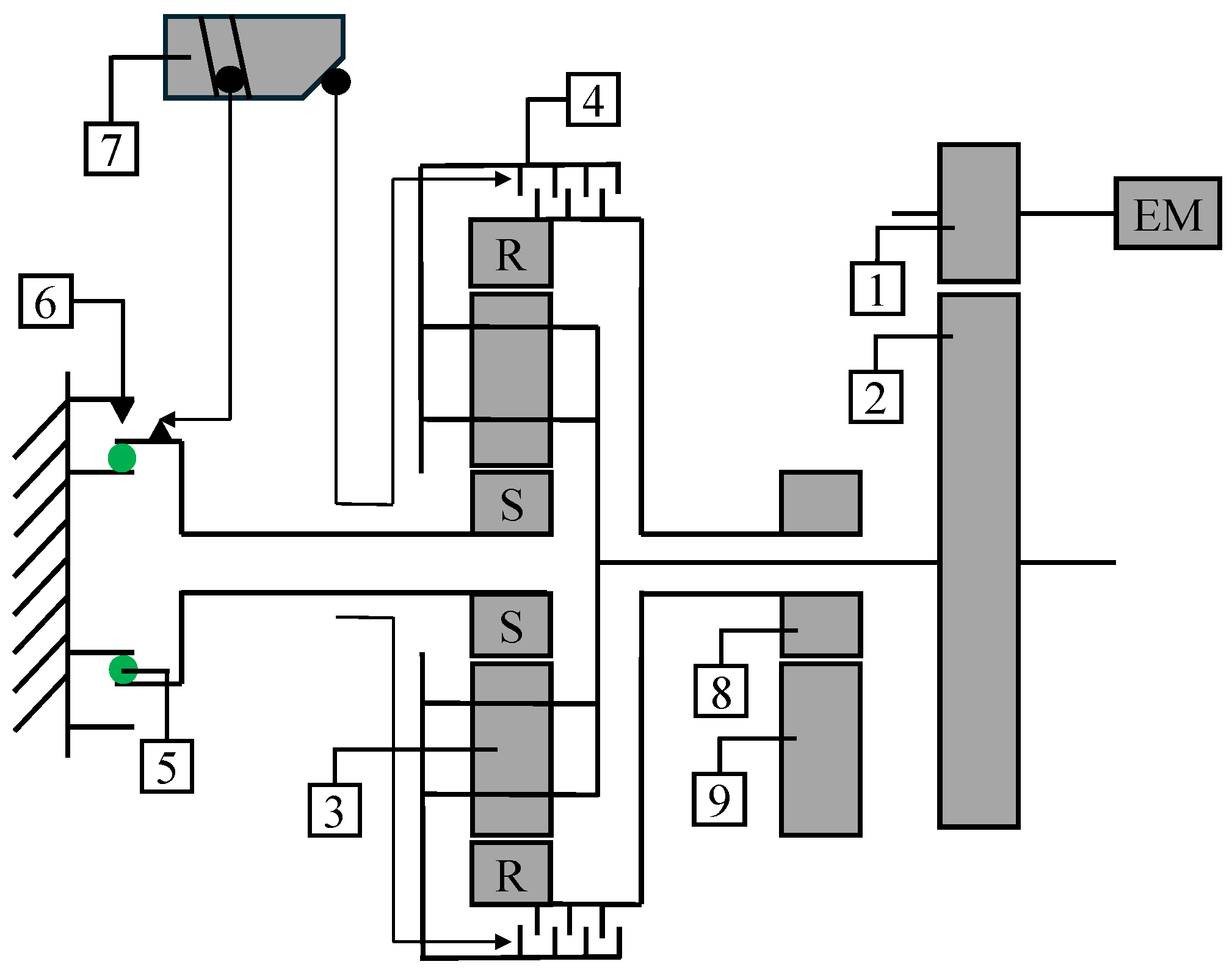
Appendix A. Vehicle Specifications

The vehicle specifications of the vehicle under study are provided in Table A1.
Table A1. Overview of vehicle specifications of the Porsche Taycan under study. Data are collected from the Certificate of Conformity (CoC) according to EU Regulation 2018/858 [38], previous material analysis in the literature [33,65], and assumptions based on media and press releases [37,39].
DomainAttributeValueUnit
VehicleRange (WLTP) c484km
Max. speed c230km/h
Mass c2205kg
Actual mass c2282kg
Test mass m2307kg
Front tyres c245/45 R 20 103Y XL-
Rear tyres c245/45 R 20 103Y XL-
Wheel rim cTaycan Turbo Aero wheel-
Tyre radius m346.8mm
RLC- f 0  c192.4N
RLC- f 1  c1.2N/(km/h)
RLC- f 2  c0.01976N/(km/h)2
Air resis.- c W  l0.22
Frontal area-A l0.22
Power
unit
Max. power c280kW
30 min power c120kW
LC max. power l350kW
Max. speed l140001/min
LC max. torque c357Nm
Drive type lPSM
Inverter lIGBT
Gear 1 ratio l15.56:1-
Gear 2 ratio l8.16:1-
Battery
unit
Gross energy c93.4kWh
Net energy l83.7kWh
Module number l33-
Cell number l396-
Cell lLG Chem E66A-
Cell format lPouch-
Cell chemistry lNMC721-
Configuration l198s2p-
m Determined by measurements.; c Taken from the Certificate of Conformity.; l Taken from the literature, i.e., Refs. [33,37,39,65].

Appendix B. UDS IDs and Physical Interpretation

All recorded signals from onboard measurements are summarized in Table A2.
Table A2. Overview of the utilized acquired signals from UDS requests via the OBD-II interface of the investigated Porsche Taycan.
Control Device NameControl Device IDSignal NameSignal IDStart-BitBit-LengthConversionUnit
Power steering0x712Steering wheel angle0x1F0F40241/2400+0°
ABS control0x713Brake pedal activation0xFD112481+0-
Accelerator pedal position0x2B2F24810/25+0%
Gear selected0x2BB82481+0-
Rear spoiler0x724Rear spoiler level0x03023281+0-
Thermal management0x742HV heater current0x475F2481/4+0A
Air intake level right0x51333281/200+0-
Air intake level left0x51343281/200+0-
Air conditioning0x746Outside temp0x26093281/10+0°C
Interior temp0x261324161/10+0°C
Rear motor0x7E0Gearbox speed output0x2C6924161+0rpm
Rear motor torque0x3E8124161/10+0Nm
Gearbox oil temp0x2C6E2481–50°C
Gearbox speed input0x2C7724161+0rpm
HV battery0x7E5State of charge0x028C2481+0%
HV pack voltage0x180124161/10+0V
HV pack current0x180224241/100–1500A
HV pack inlet temp0x181C2481–50°C
HV pack outlet temp0x181D2481–50°C
HV battery temp avg0x1E102481–100°C
Rear inverter0x17FC007CRear stator temp0x3E9424161/64+0°C
Rear inverter temp0x3E9524161/64+0°C
Gear selected neutral0x3E9B2481+0-
Chassis level0x17FC0080Chassis level0x2B942481/32+0-
Body control0x17FC008BVehicle speed0x100E32161/100+0km/h
DCDC converter0x17FC00B7HV dcdc power0x1303248100+0W
AC compressor power0x1304248100+0W
LV power0x1305248100+0W

Appendix C. Test Duration Log

All performed test durations and distances are concatenated in Table A3.
Table A3. Test recording of duration and distance. Note that only successful runs were recorded, and all aborted tests were excluded. The required time for the evaluation of the tests was recorded but not taken into account at the overall time duration since this does not represent objective results.
DescriptionTime in hDistance in km
Vehicle preparation100516
Reverse engineering and logger configuration40
Application and implementation pedal control60
Coast-down tests15457
Chassis level Medium and Lowered6
Chassis level Low9
Evaluation40
Gear shift timing27248
Upshift Normal mode12
Upshift Sport mode12
Downshift3
Evaluation15
Power unit efficiency35625
Efficiency map 1st gear18
Efficiency map 2nd gear17
Evaluation20
Official and real-driving driving cycles2598,680
Parameterization vehicle dynamometer20
Validation dynamometer setup6
Normal mode driving cycles111
Range mode driving cycles117
Individual driving cycle tests5
Evaluation120
Climate chamber tests14874
Warm-up profiles7
Constant velocity consumption7
Evaluation40
Charging measurements14-
AC Charging10
DC Charging4
Evaluation10
Total46411,400

References

  1. European Union Council. Regulation (EU) 2021/1119 of the European Parliament and of the Council of 30 June 2021 Establishing the Framework for Achieving Climate Neutrality and Amending Regulations (EC) No 401/2009 and (EU) 2018/1999 (‘European Climate Law’). 2021. Available online: http://data.europa.eu/eli/reg/2021/1119/oj (accessed on 19 February 2025).
  2. European Union Council. Regulation (EU) 2019/631 of the European Parliament and of the Council of 17 April 2019 Setting CO2 Emission Performance Standards for New Passenger Cars and for New Light Commercial Vehicles, and Repealing REGULATIONS (EC) No 443/2009 and (EU) No 510/2011. 2019. Available online: https://eur-lex.europa.eu/eli/reg/2019/631/oj (accessed on 19 February 2025).
  3. Kampker, A. Elektromobilität: Grundlagen Einer Fortschrittstechnologie; Springer: Berlin/Heidelberg, Germany, 2024. [Google Scholar] [CrossRef]
  4. Fritz, A.; Verband der Automobilindustrie e.V. (VDA). E-Mobility Globally on the Rise. 2024. Available online: https://www.vda.de/en/topics/electromobility/market-developments-europe-international (accessed on 19 February 2025).
  5. Statista, Inc. Market Share of Electric Vehicles in Germany from 2014 to 2024. 2024. Available online: https://www.statista.com/statistics/1166826/electric-vehicles-market-share-germany/ (accessed on 19 February 2025).
  6. Nationale Plattform Zukunft der Mobilität. Customer Acceptance as the Key to the Market Ramp-Up of Electromobility. 2024. Available online: https://www.plattform-zukunft-mobilitaet.de/en/2download/customer-acceptance-as-the-key-to-the-market-ramp-up-of-electromobility-german-report/ (accessed on 20 February 2025).
  7. Rudschies, W.; Allgemeiner Deutscher Automobil-Club (ADAC) e.V. Fakten zur Elektromobilität: Das sind die Vor- und Nachteile. 2023. Available online: https://www.adac.de/rund-ums-fahrzeug/elektromobilitaet/elektroauto/elektroauto-pro-und-contra/ (accessed on 20 February 2025).
  8. Rosenberger, N.; Fundel, M.; Bogdan, S.; Köning, L.; Kragt, P.; Kühberger, M.; Lienkamp, M. Scientific benchmarking: Engineering quality evaluation of electric vehicle concepts. e-Prime-Adv. Electr. Eng. Electron. Energy 2024, 9, 100746. [Google Scholar] [CrossRef]
  9. Lienert, P. Reuters. Exclusive: Automakers to Double Spending on EVs, Batteries to $1.2 Trillion by 2030. 2022. Available online: https://www.reuters.com/technology/exclusive-automakers-double-spending-evs-batteries-12-trillion-by-2030-2022-10-21/ (accessed on 20 February 2025).
  10. Bank Vontobel Europe, AG. Der Markt für Elektrofahrzeuge Ist Hart Umkämpft. 2022. Available online: https://www.boerse.de/nachrichten/Der-Markt-fuer-Elektrofahrzeuge-ist-hart-umkaempft-Werbung/33467234 (accessed on 20 February 2025).
  11. Doppelbauer, M. Grundlagen der Elektromobilität: Technik, Praxis, Energie und Umwelt; Springer: Wiesbaden, Germany, 2020. [Google Scholar] [CrossRef]
  12. Rimac Automobili. Rimac Nevera. 2021. Available online: https://www.rimac-automobili.com/nevera/ (accessed on 20 February 2025).
  13. Jordan, M. MBpassion. Fahrwerk & Getriebe des G 580 mit EQ Technologie. 2024. Available online: https://mbpassion.de/2024/04/fahrwerk-getriebe-des-g-580-mit-eq-technologie/ (accessed on 20 February 2025).
  14. Porsche Newsroom. The Powertrain: Pure Performance. 2019. Available online: https://newsroom.porsche.com/en/products/taycan/powertrain-18555.html/ (accessed on 20 February 2025).
  15. Machado, F.A.; Kollmeyer, P.J.; Barroso, D.G.; Emadi, A. Multi-Speed Gearboxes for Battery Electric Vehicles: Current Status and Future Trends. IEEE Open J. Veh. Technol. 2021, 2, 419–435. [Google Scholar] [CrossRef]
  16. Störiko, A. HIGHEST–Innovations-und Gründungszentrum. Effizientere E-Autos dank Gangschaltung. 2024. Available online: https://highest-darmstadt.de/de/news/unkategorisiert/effizientere-e-autos-dank-gangschaltung/ (accessed on 20 February 2025).
  17. Laitinen, H.; Lajunen, A.; Tammi, K. Improving Electric Vehicle Energy Efficiency with Two-Speed Gearbox. In Proceedings of the 2017 IEEE Vehicle Power and Propulsion Conference (VPPC), Belfort, France, 11–14 October 2017; pp. 1–5. [Google Scholar] [CrossRef]
  18. Köllner, C. Etabliert sich die 800-V-Systemarchitektur im Massenmarkt? Springer, 2024. Available online: https://www.springerprofessional.de/elektrofahrzeuge/antriebsstrang/etabliert-sich-die-800-v-systemarchitektur-im-massenmarkt-/26653216/ (accessed on 20 February 2025).
  19. Greenhalgh, K. Transport Topics. Tesla Promises Semi Truck Production to Begin in Late 2025. 2024. Available online: https://www.ttnews.com/articles/tesla-semi-truck-2025/ (accessed on 20 February 2025).
  20. Blomgren, G.E. The Development and Future of Lithium Ion Batteries. J. Electrochem. Soc. 2017, 164, A5019–A5025. [Google Scholar] [CrossRef]
  21. Momen, F.; Rahman, K.; Son, Y. Electrical propulsion system design of Chevrolet Bolt battery electric vehicle. IEEE Trans. Ind. Appl. 2018, 55, 376–384. [Google Scholar] [CrossRef]
  22. Sarlioglu, B.; Morris, C.T.; Han, D.; Li, S. Benchmarking of electric and hybrid vehicle electric machines, power electronics, and batteries. In Proceedings of the 2015 Intl Aegean Conference on Electrical Machines & Power Electronics (ACEMP), 2015 Intl Conference on Optimization of Electrical & Electronic Equipment (OPTIM) & 2015 Intl Symposium on Advanced Electromechanical Motion Systems (ELECTROMOTION), Side, Turkey, 2–4 September 2015; pp. 519–526. [Google Scholar] [CrossRef]
  23. Kovachev, G.; Schröttner, H.; Gstrein, G.; Aiello, L.; Hanzu, I.; Wilkening, H.M.R.; Foitzik, A.; Wellm, M.; Sinz, W.; Ellersdorfer, C. Analytical Dissection of an Automotive Li-Ion Pouch Cell. Batteries 2019, 5, 67. [Google Scholar] [CrossRef]
  24. Löbberding, H.; Wessel, S.; Offermanns, C.; Kehrer, M.; Rother, J.; Heimes, H.; Kampker, A. From Cell to Battery System in BEVs: Analysis of System Packing Efficiency and Cell Types. World Electr. Veh. J. 2020, 11, 77. [Google Scholar] [CrossRef]
  25. Oh, G.; Leblanc, D.J.; Peng, H. Vehicle Energy Dataset (VED), A Large-Scale Dataset for Vehicle Energy Consumption Research. IEEE Trans. Intell. Transp. Syst. 2020, 23, 3302–3312. [Google Scholar] [CrossRef]
  26. Diez, J. Advanced Vehicle Testing and Evaluation, Final Technical Report Encompassing Project Activities from 1 October 2011 to 30 April 2018; Technical Report; Intertek Testing Services, NA, Inc.: Arlington Heights, IL, USA, 2018. [Google Scholar] [CrossRef]
  27. Wassiliadis, N.; Steinsträter, M.; Schreiber, M.; Rosner, P.; Nicoletti, L.; Schmid, F.; Ank, M.; Teichert, O.; Wildfeuer, L.; Schneider, J.; et al. Quantifying the state of the art of electric powertrains in battery electric vehicles: Range, efficiency, and lifetime from component to system level of the Volkswagen ID.3. eTransportation 2022, 12, 100167. [Google Scholar] [CrossRef]
  28. Rosenberger, N.; Rosner, P.; Bilfinger, P.; Schöberl, J.; Teichert, O.; Schneider, J.; Abo Gamra, K.; Allgäuer, C.; Dietermann, B.; Schreiber, M.; et al. Quantifying the State of the Art of Electric Powertrains in Battery Electric Vehicles: Comprehensive Analysis of the Tesla Model 3 on the Vehicle Level. World Electr. Veh. J. 2024, 15, 268. [Google Scholar] [CrossRef]
  29. EV Database. Porsche Taycan. 2021. Available online: https://ev-database.org/car/1393/Porsche-Taycan (accessed on 11 February 2025).
  30. EV Database. Porsche Taycan 4S. 2020. Available online: https://ev-database.org/car/1237/Porsche-Taycan-4S (accessed on 11 February 2025).
  31. EV Database. Porsche Taycan GTS. 2022. Available online: https://ev-database.org/car/1560/Porsche-Taycan-GTS (accessed on 11 February 2025).
  32. EV Database. Porsche Taycan Turbo. 2020. Available online: https://ev-database.org/car/1229/Porsche-Taycan-Turbo (accessed on 11 February 2025).
  33. EV Database. Porsche Taycan Plus. 2021. Available online: https://ev-database.org/car/1394/Porsche-Taycan-Plus (accessed on 11 February 2025).
  34. EV Database. Porsche Taycan Sport Turismo. 2022. Available online: https://ev-database.org/car/1621/Porsche-Taycan-Sport-Turismo (accessed on 11 February 2025).
  35. EV Database. Porsche Taycan 4 Cross Turismo. 2021. Available online: https://ev-database.org/car/1186/Porsche-Taycan-4-Cross-Turismo (accessed on 11 February 2025).
  36. EV Database. Porsche Taycan Turbo GT. 2024. Available online: https://ev-database.org/car/2144/Porsche-Taycan-Turbo-GT (accessed on 11 February 2025).
  37. Porsche Newsroom. Technical Data: Taycan with Performance Battery/Taycan with Performance Battery Plus. 2022. Available online: https://press.cee.porsche.com/prod/presse_pag/PressResources.nsf/Content?ReadForm&languageversionid=1364534&hl=modelle-missione-concept (accessed on 11 February 2025).
  38. European Parliament. Regulation (EU) 2018/858 of the European Parliament and of the Council of 30 May 2018 on the Approval and Market Surveillance of Motor Vehicles and Their Trailers, and of Systems, Components and Separate Technical Units Intended for Such Vehicles, Amending Regulations (EC) No 715/2007 and (EC) No 595/2009 and Repealing Directive 2007/46/EC. 2018. Available online: https://eur-lex.europa.eu/eli/reg/2018/858/oj (accessed on 15 January 2025).
  39. Porsche Newsroom. Aerodynamics: The Best Value of All Current Porsche Models. 2022. Available online: https://newsroom.porsche.com/en_US/products/taycan/aerodynamics-18554.html (accessed on 11 February 2025).
  40. Porsche Newsroom. Greater Driving Precision, Driving Dynamics and Driving Comfort. 2022. Available online: https://newsroom.porsche.com/en/press-kits/taycan/Das-Fahrwerk.html (accessed on 11 February 2025).
  41. The European Comission. Commission Regulation (EU) 2017/1151 of 1 June 2017 Supplementing Regulation (EC) No 715/2007 of the European Parliament and of the Council on Type-Approval of Motor Vehicles with Respect to Emissions from Light Passenger and Commercial Vehicles (Euro 5 and Euro 6) and on Access to Vehicle Repair and Maintenance Information, Amending Directive 2007/46/EC of the European Parliament and of the Council, Commission Regulation (EC) No 692/2008 and Commission Regulation (EU) No 1230/2012 and Repealing Commission Regulation (EC) No 692/2008. 2017. Available online: https://eur-lex.europa.eu/legal-content/EN/TXT/?uri=CELEX%3A02017R1151-20230901 (accessed on 7 December 2024).
  42. United Nations. Global Technical Regulation on Worldwide Harmonized Light Vehicles Test Procedure. Addendum 15: Global Technical Regulation No. 15 (ECE/TRAN/180/Add.15). 2014. Available online: https://unece.org/fileadmin/DAM/trans/main/wp29/wp29r-1998agr-rules/ECE-TRANS-180a15e.pdf (accessed on 4 January 2025).
  43. Merkle, L.; Pöthig, M.; Schmid, F. Estimate e-Golf Battery State Using Diagnostic Data and a Digital Twin. Batteries 2021, 7, 15. [Google Scholar] [CrossRef]
  44. Rosenberger, N.; Lienkamp, M. Vehicle Parameter and Electric Powertrain Efficiency Analysis Using Real-Driving Data. Int. J. Electr. Electron. Eng. Telecommun. 2024, 13, 494–502. [Google Scholar] [CrossRef]
  45. The European Comission. Comission Regulation (EU) 2018/1832. 2018. Available online: https://climate.ec.europa.eu/eu-action/transport-emissions/road-transport-reducing-co2-emissions-vehicles/co2-emission-performance-standards-cars-and-vans_en (accessed on 7 May 2023).
  46. Sarkan, B.; Skrucany, T.; Semanova, S.; Madlenak, R.; Kuranc, A.; Sejkorova, M.; Caban, J. Vehicle coast-down method as a tool for calculating total resistance for the purposes of type-approval fuel consumption. Sci. J. Silesian Univ. Technol. 2018, 98, 11. [Google Scholar] [CrossRef]
  47. Box, G.E.P.; Jenkins, G.M. Time Series Analysis: Forecasting and Control; Holden-Day: San Francisco, CA, USA, 1970. [Google Scholar]
  48. Alami, A.; Belmajdoub, F. Noise Reduction Techniques in Adas Sensor Data Management: Methods and Comparative Analysis. Int. J. Adv. Comput. Sci. Appl. 2024, 15, 679. [Google Scholar] [CrossRef]
  49. Rohde-Brandenburger, K. Verbrauch in Fahrzyklen und im Realverkehr. In Energiemanagement im Kraftfahrzeug: Optimierung von CO2-Emissionen und Verbrauch konventioneller und Elektrifizierter Automobile; Springer Fachmedien Wiesbaden: Wiesbaden, Germany, 2014; pp. 243–306. [Google Scholar] [CrossRef]
  50. United States Environmental Protection Agency. Data on Cars Used for Testing Fuel Economy-2021 Test Car List Data. 2022. Available online: https://www.epa.gov/compliance-and-fuel-economy-data/data-cars-used-testing-fuel-economy (accessed on 4 January 2025).
  51. Qi, H.; Chen, Y.; Zhang, N.; Zhang, B.; Wang, D.; Tan, B. Improvement of both handling stability and ride comfort of a vehicle via coupled hydraulically interconnected suspension and electronic controlled air spring. Proc. Inst. Mech. Eng. Part J. Automob. Eng. 2020, 234, 552–571. [Google Scholar] [CrossRef]
  52. Busch, R.; Beck, M. Elektrotechnik und Elektronik: Für Maschinenbauer und Verfahrenstechniker; Springer: Wiesbaden, Germany, 2024. [Google Scholar] [CrossRef]
  53. Tschöke, H.; Gutzmer, P.; Pfund, T. Elektrifizierung des Antriebsstrangs: Grundlagen-vom Mikro-Hybrid zum Vollelektrischen Antrieb; Springer: Wiesbaden, Germany, 2019. [Google Scholar] [CrossRef]
  54. Koch, A. Energieeffizientes Fahren und Optimale, Elektrische Antriebsstränge für Automatisierte Fahrzeuge. Ph.D. Thesis, Technical University of Munich, Munich, Germany, 2022. [Google Scholar]
  55. Binder, A. Elektrische Maschinen und Antriebe: Grundlagen, Betriebsverhalten; Springer: Wiesbaden, Germany, 2018. [Google Scholar] [CrossRef]
  56. United States Environmental Protection Agency. Fuel Economy and EV Range Testing. 2024. Available online: https://www.epa.gov/greenvehicles/fuel-economy-and-ev-range-testing (accessed on 4 January 2025).
  57. Liu, Y.; Wu, Z.X.; Zhou, H.; Zheng, H.; Yu, N.; An, X.P.; Li, J.Y.; Li, M.L. Development of China Light-Duty Vehicle Test Cycle. Int. J. Automot. Technol. 2020, 21, 1233–1246. [Google Scholar] [CrossRef]
  58. United States Environmental Protection Agency. EPA SC03 Supplemental Federal Test Procedure (SFTP) with Air Conditioning. 2024. Available online: https://www.epa.gov/emission-standards-reference-guide/epa-sc03-supplemental-federal-test-procedure-sftp-air (accessed on 4 January 2025).
  59. Allgemeiner Deutscher Automobil-Club (ADAC) e.V. Porsche Taycan 4S Performancebatterie Plus (01/20–02/24). 2020. Available online: https://www.adac.de/rund-ums-fahrzeug/autokatalog/marken-modelle/porsche/taycan/y1a/305473/#eco-test (accessed on 23 January 2025).
  60. Küçükay, F. Grundlagen der Fahrzeugtechnik: Antriebe, Getriebe, Energieverbrauch, Bremsen, Fahrdynamik, Fahrkomfort; Springer: Wiesbaden, Germany, 2020. [Google Scholar] [CrossRef]
  61. Lightshape GmbH & Co. KG. Porsche Mission E: 3D Animation/Product Vizualization/Realfilm. 2022. Available online: https://www.lightshape.net/en/projects/porsche-mission-e-drive-movie (accessed on 23 January 2025).
  62. Aghabali, I.; Bauman, J.; Kollmeyer, P.J.; Wang, Y.; Bilgin, B.; Emadi, A. 800-V Electric Vehicle Powertrains: Review and Analysis of Benefits, Challenges, and Future Trends. IEEE Trans. Transp. Electrif. 2021, 7, 927–948. [Google Scholar] [CrossRef]
  63. Snyder, J. autoblog. Here Are All the EVs with 800 V Charging Available in 2024. 2024. Available online: https://www.autoblog.com/news/800-volt-electric-vehicles-list (accessed on 23 January 2025).
  64. Specht, K.; Gall, M.; Scheidhammer, G. Von 400 auf 800 V–Auswirkungen auf das Hochvoltbordnetz. ATZ Elektron 2019, 14, 42–45. [Google Scholar] [CrossRef]
  65. Batemo. Batemo Cell Explorer–LG Chem E66A. 2022. Available online: https://www.batemo.com/products/batemo-cell-explorer/lg-chem-e66a/#get-model-popup (accessed on 24 February 2025).
Figure 1. This study’s layout with its objectives allocated to their respective sections as an overview.
Wevj 16 00296 g001
Figure 2. Comparison of the experimentally derived coast-down curves: (a) in chassis levels, Medium, Lowered, and Low, where Low represents the Range mode curve, and the combination of Medium and Lowered represents the Normal mode curve; (b) in Normal and Range modes compared to the official test results in the CoC [38] and the EPA [50].
Wevj 16 00296 g002
Figure 3. Comparison of the driving resistances derived from RLCs based on experimentally recorded coast-down curves and RLCs of official test results in the CoC and the EPA. Note that the dashed lines represent extrapolated data, since the actual measurements were recorded according to Table 1.
Wevj 16 00296 g003
Figure 4. Gear shift timing in Normal and Sport modes (a) at different motor torques, (b) at different mechanical power levels.
Wevj 16 00296 g004
Figure 5. Efficiency characteristics of the power unit, consisting of the inverter, electric machine, and transmission, in (a) first gear, created with 174 discrete measurement points, and in (b) second gear, created with 223 discrete measurement points through recorded onboard data. Measurement points are illustrated as crosses.
Wevj 16 00296 g005
Figure 6. Efficiency map overlay between the power unit’s first and second gear.
Wevj 16 00296 g006
Figure 7. Maximum achievable range in international test procedures (black) compared to real-world cycles (blue) in Normal (primary driving mode) and Range mode. Note that all experiments were performed by continuously driving the vehicle until it could no longer follow the target velocity.
Wevj 16 00296 g007
Figure 8. Comparison of the WLTC range between the two driving resistances and driving modes on the dynamometer derived from the average of three driven test cycles.
Wevj 16 00296 g008
Figure 9. Warm-up behavior of the vehicle under study at three different temperature levels during the WLTC.
Wevj 16 00296 g009
Figure 10. Experimentally determined energy consumption and electric ranges at constant speed levels. Energy consumption (a) is measured at discrete intervals, and (b) extrapolated with the extractable energy in the WLTC scenario, gaining the maximum achievable range of the vehicle.
Wevj 16 00296 g010
Figure 11. Schematic of the two-speed transmission in the Porsche Taycan: (1) parallel spur gear pair 1-pinion (input) from the electric machine (EM), (2) parallel spur gear pair 1-gear, (3) planetary gear set, planet gears (S: sun gear, R: ring gear), (4) multi-plate clutch, (5) freewheel, (6) dog clutch, (7) shift drum with ball ramp mechanism, (8) parallel spur gear pair 2-pinion (output), (9) parallel spur gear pair 2-gear based on [60].
Wevj 16 00296 g011
Figure 12. Efficiency optimization through load point switch from (a) first gear to the compromise gear and (b) from second gear to compromise gear (ID.3 gear ratio). Deviation between the efficiency maps in %.
Wevj 16 00296 g012
Figure 13. Energy losses of the vehicle under study during one cycle run of the two official driving cycles and the three real-world driving based cycles: (a) shows the absolute energy losses and (b) the relative energy share losses. The energy losses not visible in the figure are shown in Table 5.
Wevj 16 00296 g013
Figure 14. Comparison between the Volkswagen ID.3 and the vehicle under study in (a) charging power in kW and the charged energy in kWh and (b) the temperature in °C. The dotted lines indicate results of the Volkswagen ID.3 [27].
Wevj 16 00296 g014
Table 1. Vehicle speed segments according to the chassis levels.
MediumLoweredLow
100–80 km/h165–150 km/h165–145 km/h
85–70 km/h155–135 km/h150–135 km/h
75–60 km/h140–120 km/h140–125 km/h
65–45 km/h120–105 km/h130–115 km/h
50–30 km/h110–95 km/h120–105 km/h
35–0 km/h100–85 km/h110–95 km/h
85–65 km/h100–75 km/h
70–50 km/h90–75 km/h
55–30 km/h80–55 km/h
35–0 km/h60–45 km/h
Table 2. Comparison of the RLCs derived from the performed coast-down test and the RLCs given by the CoC [38] and the EPA [50].
Parameter (Unit) f 0 (N) f 1 (N/(km/h)) f 2 (N/(km/h)2)
Low = Range173.90.0050.02871
Lowered188.70.0640.02989
Medium138.41.9810.01456
Normal164.30.6980.02649
CoC192.41.2000.01976
EPA169.71.2000.02240
Table 3. Comparison between the two-speed transmission of the vehicle under study and the single-speed transmission of the Volkswagen ID.3 [27].
Two-Speed TransmissionSingle-Speed Transmission
Component Name Mass in kg Component Name Mass in kg
Housing (3-piece)26.05Housing (2-piece)9.90
Differential16.50Differential9.95
Input shaft0.90Input shaft1.49
Inner shaft3.80Intermediate shaft2.12
Outer shaft1.70Output shaft1.05
Ring gear2.50
Planet carrier3.70
Sun gear0.90
Planet gears1.05
Multi-plate clutch2.70
Dog clutch2.20
Total mass62.00Total mass24.51
Table 4. Overview of the energy consumption of the first and second gears’ transferred load points in the compromise gear.
Test CycleEnergy Consumption in kWhEnergy Consumption in kWh
1st Gear Compromise Gear Difference in % 2nd Gear Compromise Gear Difference in %
WLTC2.6322.595−1.421.9481.999+2.54
FTP-752.9662.932−1.170.61410.6353+3.35
HWFET0.48710.4809−1.291.8751.957+4.2
Urban1.4901.480−0.6400-
Interurban2.3572.3401−0.721.5611.623+3.83
Highway1.0351.025−0.977.3097.446+1.84
Table 5. Comparison between the absolute energy losses in kWh of the Volkswagen ID.3 and the vehicle under study. The suffices P indicate results of the Porsche and VW results for the Volkswagen ID.3 [27]. The numbers in the parentheses indicate the relative energy losses in %.
Test Cycle E Ohm E Aux E ItW E WtD E total
WLTC-P0.03 (0.83)0.25 (6.89)0.89 (24.03)2.54 (68.35)3.72
WLTC-VW0.06 (1.99)0.14 (4.41)0.67 (21.01)2.33 (72.59)3.20
FTP-75-P0.02 (0.77)0.26 (9.61)1.01 (37.11)1.43 (52.51)2.72
FTP-75-VW0.03 (1.64)0.15 (7.61)0.51 (25.91)1.29 (64.84)1.99
Urban-P0.01 (0.56)0.16 (13.29)0.53 (43.33)0.52 (42.82)1.21
Urban-VW0.01 (1.23)0.08 (10.57)0.25 (31.49)0.46 (56.71)0.80
Interurban-P0.04 (1.20)0.20 (6.66)0.88 (28.85)1.92 (63.29)3.04
Interurban-VW0.07 (2.73)0.11 (4.50)0.45 (18.55)1.78 (74.22)2.40
Highway-P0.12 (1.61)0.20 (2.69)0.64 (7.29)5.40 (88.41)7.35
Highway-VW0.29 (3.96)0.21 (2.86)0.86 (11.18)6.02 (82.01)7.31
Disclaimer/Publisher’s Note: The statements, opinions and data contained in all publications are solely those of the individual author(s) and contributor(s) and not of MDPI and/or the editor(s). MDPI and/or the editor(s) disclaim responsibility for any injury to people or property resulting from any ideas, methods, instructions or products referred to in the content.

