Three-Dimensional Unmanned Aerial Vehicle Path Planning in Simulated Rugged Mountainous Terrain Using Improved Enhanced Snake Optimizer (IESO)

Abstract

The challenging terrain and deep ravines that characterize mountainous regions often result in slower path planning and suboptimal flight paths for unmanned aerial vehicles (UAVs) when traditional meta-heuristic optimization algorithms are employed. This study proposes a novel Improved Enhanced Snake Optimizer (IESO) for three-dimensional path planning and tested it in a simulated rugged mountainous terrain with obstacles and a restricted “no-fly zone”. The initialization process in the enhanced snake optimizer is refined by integrating the Chebyshev chaotic map. Additionally, a non-monotonic factor is introduced to modulate the “temperature”. This temperature controls the freedom of movement within the solution space. Furthermore, a boundary condition is incorporated into the dynamic opposition learning mechanism. These modifications collectively reduce the likelihood of population convergence to local optima during optimization. The feasibility of IESO is validated through time complexity and global convergence analyses. Comparative simulation experiments benchmarked IESO against five state-of-the-art biologically inspired optimization algorithms across test functions and path-planning simulated scenarios. Experimental results show that compared with five commonly used algorithms, the IESO algorithm improves the quality of flight trajectory planning by nearly 30% on average. Particularly when compared to the original SO algorithm, IESO demonstrates performance enhancement exceeding 36%, proving its superiority in UAV path planning over complex terrain.

1. Introduction

Path planning plays a crucial role in ensuring fast and stable flight for unmanned aerial vehicles (UAVs) during monitoring and inspection tasks [1]. Complex mountainous terrains, characterized by significant elevation changes and limited transportation options, often render certain areas difficult to access using conventional observation, surveillance, and logistical support methods. Due to their agility and flexibility, UAVs have become extensively utilized in these challenging environments. Consequently, high-quality and rapid flight path planning in such complex terrains is critically important for enhancing the efficiency of UAV missions [2,3].

Recent research in UAV path planning has introduced a range of methodologies, including meta-heuristic optimization algorithms (MAs) [4], a quality-oriented hybrid A* and Q-learning algorithm [5], the artificial potential field method [6], and trajectory planning using Dijkstra’s matrix-aligned algorithm [7,8]. Flores-Caballero et al. [9] approached path planning as a constrained global optimization problem, combining MAs with the A* algorithm. Lin and Liu [10] had an improved A* algorithm for driverless vehicle path planning. He et al. [11] proposed a new path planning approach for complex environments using the A* algorithm. Shao et al. [12] developed a hierarchical trajectory optimization framework that integrates adaptive particle swarm optimization with the Gaussian pseudospectral method. For large-scale collaborative searches, Chen et al. [13] utilized the ant colony optimization algorithm to efficiently plan UAV swarm paths and reduce task completion times. Fu et al. [14] introduced a multi-UAV multilayer projection clustering (MMPC) algorithm that minimizes the cumulative distance between multilayer targets and their respective cluster centers in environments with complex obstacles. They later improved this method using a probabilistic road map to reduce zigzagging around path endpoints, particularly in congestion-prone areas [15]. Zhao et al. [16] reported a simulated result on autonomous path planning for obstacle avoidance in Gazebo, particularly in unfamiliar environments.

In a recent review, Luo et al. [17] categorized UAV path planning algorithms into two main levels, algorithmic and functional, each with three subcategories. The algorithmic level includes traditional, intelligent, and hybrid algorithms, while the functional level comprises space-based, time-based, and task-based approaches. A similar classification was proposed by Wang and Pan back in 2021 [18]; they named their proposed categories as follows: traditional, intelligent, and fusion algorithms.

In another review, Debnath et al. [19] used two major categories: the global and local in a single UAV and multi-UAV. Luo’s classification is more about the algorithm, while Debnath focuses on UAV number and obstacle avoidance.

According to Luo’s classification, our Improved Enhanced Snake Optimizer (IESO) is a biologically inspired swarm intelligence algorithm designed for rugged mountainous terrains. Characterized by medium complexity, medium–high fault tolerance, moderate–fast computational speeds, and medium–high robustness and reliability, the method aligns with typical biologically inspired algorithm characteristics. Following Debnath’s classification, it represents a single-UAV path planning and obstacle avoidance approach, specifically addressing challenges posed by terrain elevation changes and restricted “no-fly zones”.

In our study, we examined the Enhanced Snake Optimizer (ESO) proposed by Yao et al. [20], which builds upon the original Snake Optimizer (SO) developed by Hashim and Hussien [21]. The Enhanced Snake Optimizer (ESO) introduces enhancements such as randomized population initialization and mirror imaging. These have been validated using classical tests and engineering design functions. The results demonstrate the algorithm’s potential for UAV path planning. However, consistent with the No Free Lunch theorem [22], which states that no single algorithm is optimal for all optimization problems, we acknowledge the inherent limitations of ESO. For our IESO, we aim to improve on optimization precision, particularly in global optima, convergence speed, short length, and high quality of the flight path for UAV; this means that we aim to achieve the shortest distance with a smooth path in a 3D complex environment with obstacles and a “no-fly zone”.

We evaluated IESO against five state-of-the-art biologically inspired algorithms: SO [21], ESO [20], Golden Jackal Optimization (GJO) [23,24], Honey Badger Algorithm (HBA) [25], and Grey Wolf Optimizer (GWO) [26]. Our results demonstrate that IESO outperforms all five in terms of precision, convergence speed, and overall trajectory quality.

The SO algorithm mimics the dynamic predator–prey behavior, balancing exploration and exploitation, with a “temperature” parameter controlling the solution space search dynamics [21]; while this is effective for continuous optimization, it suffers from premature convergence and sensitivity to parameter tuning [27,28]. In Zheng et al. [29], Sobol sequential nonlinear factors and different learning strategies were proposed to improve the SO from a purely mathematical perspective.

ESO improves upon SO by introducing diversification and intensification mechanisms, which enhance accuracy and robustness. However, these benefits come at the cost of higher computational demands and greater sensitivity to parameter settings. A few improved or enhanced SO algorithms have been proposed [30,31], which focus on improving the algorithm, but they are not specific for UAV path planning.

GJO, inspired by the hunting strategies of golden jackals, incorporates adaptive weight factors that allow dynamic control over convergence. Although it shows strong exploratory capabilities, it suffers from slow convergence and limited robustness [32].

HBA is a population-based metaheuristic optimization algorithm derived from two-phase search behaviors: pressure and digging. It performs well in relatively complex environments by escaping local optima. However, it is computationally expensive, does not scale efficiently, and shows the imbalance between exploration and exploitation. Some instability has also been reported on standard benchmark functions [33].

GWO is based on a leadership hierarchy and collective hunting behavior [24]. It has demonstrated effective global search capability, but struggles with slow convergence and premature convergence in highly complex scenarios [34].

We found that the current path planning approaches, particularly meta-heuristic optimization, often result in slower path planning and suboptimal trajectories in complex mountainous environments, particularly where obstacles and no-fly zones are present. They also suffer from premature convergence to local optima, or at least not in a robust and stable manner. The biologically inspired algorithms lacked enhancement in balancing the exploration and exploitation effectively for rugged terrains.

To address these limitations, we propose three significant enhancements to ESO, resulting in the Improved Enhanced Snake Optimizer (IESO), which is particularly well suited for rugged terrain models. The main contributions of this work are as follows: (1) Proposal of the Improved Enhanced Snake Optimizer (IESO) algorithm, which demonstrates its enhanced capability for global search and improved convergence speed in complex 3D path planning problems. (2) Comprehensive evaluation of IESO against classical and state-of-the-art swarm intelligence algorithms, showing superior performance in flight trajectory optimization for unmanned aerial vehicles (UAVs) in simulated rugged mountainous terrain. (3) Successful application of IESO to UAV path planning in three-dimensional environments, resulting in safer, more efficient trajectories with better obstacle avoidance and shorter flight distances.

2. Methodologies: Improved Enhanced Snake Optimizer (IESO) Algorithm and Simulation Design

This section is organized into four subsections: Section 2.1 briefly reviews the Snake Optimizer (SO). Section 2.2 presents a concise overview of the Enhanced Snake Optimizer (ESO). Section 2.3 offers a detailed explanation of our Improved Enhanced Snake Optimizer (IESO). Section 2.4 discusses the design of the simulation experiments and the evaluation criteria.

2.1. Fundamental Principles of Snake Optimizer (SO)

The Snake Optimizer (SO) was initially proposed by Hashim and Hussien [21] in 2022. SO is an advanced optimization algorithm inspired by the mating behavior of snakes. Its functionality is primarily influenced by environmental factors, specifically temperature and food availability. The algorithm operates in two distinct phases: exploration, where it conducts a global search for solutions, and exploitation, focusing on a local search for optimal solutions.

Mating behavior within this model is dependent on temperature, occurring mainly in cooler conditions when food is plentiful. The algorithm uses a probabilistic approach to dictate mating interactions, which include both inter-sex mating and competitive behaviors among males. This interaction is governed by a random probability threshold, determining the nature and occurrence of reproductive behaviors.

In the SO algorithm, the term “population” (N) signifies the collection of search points under consideration. These points are initialized by randomly sampling from a uniform distribution, as mathematically described in Equation (1). Subsequently, this initial population is partitioned into two equally sized subgroups: males and females.

$$X_i=X_{min}+ran{d}_i\times (X_{max}-X_{min})$$

(1)

Within the SO algorithm, the “temperature” parameter (T) governs the transition between exploration (global search) and exploitation (local search) phases. Its value is computed using Equation (2), where t represents the present iteration count, and T signifies the maximum number of iterations; this notation remains consistent throughout this document.

$$Temp=ex{p}^{-\mathit{t}/T}$$

(2)

The SO uses a dynamic search strategy where the “food” parameter represents feature positions. Under resource-limited conditions, the algorithm conducts a global search. As environmental conditions change, it adaptively refines search points, transitioning between exploration and exploitation phases. During different temperature states, search agents strategically select optimal solutions, with food quantity (defined in Equation (3)) guiding the algorithm’s precision in navigating complex solution spaces.

$$Q=c_{1}ex{p}^{(t-T)/T},c_1=0.5$$

(3)

During the foraging stage, specifically when Q falls below 0.25, individual snakes explore the search space by randomly choosing a location and adjusting their current position accordingly. This exploratory behavior is mathematically formulated for males in Equation (4), where $A_m$ is defined as Equation (5). The corresponding formulation for females mirrors the male version, with the sole distinction being the substitution of the subscript ${}_m$${–}_f$.

$$X_{i,m}(t+1)=X_{rand,m}\left(t\right)\pm c_2\times A_m\times ((X_{max}-X_{min})\times rand+X_{min}),c_2=0.05$$

(4)

$$A_m=ex{p}^{(-f_{rand,m}/f_{i,m})}$$

(5)

During the search process, when both Q and T exceed 0.6, the snake maintains a global exploration strategy to locate food. This behavior is mathematically represented in Equation (6).

$$X_{i,j}(t+1)=X_{food}\pm c_3\times Temp\times rand\times ((X_{food}-X_{i,j}\left(t\right)),c_3=2$$

(6)

where $X_{i,j}$ is the ith snake position (male or female) and $X_{food}$ is the position of the food.

If Q remains above 0.6 while T falls below 0.6, the snake transitions into either flight mode (FM) or mating mode (MM). This signifies that the search agents are undergoing a process of convergence and divergence, as detailed in Equations (7) and (8).

$$X_{i,m}(t+1)=X_{i,m}\left(t\right)+c_3\times FM\times rand\times Q\times X_{best,f}-X_{i,m}\left(t\right)),c_3=2$$

(7)

$$X_{i,f}(t+1)=X_{i,f}(t+1)+c_3\times FF\times rand\times Q\times X_{best,m}-X_{i,f}(t+1),c_3=2$$

(8)

where $X_{i,m}$ is the ith male position, $X_{best,f}$ refers to the best female position. FM and FF are the fighting ability of a snake (male and female), and it is defined in Equations (9) and (10).

$$\mathrm{FM}={exp}^{-f_{best,f}/f_i}$$

(9)

$$\mathrm{FF}={exp}^{-f_{best,m}/f_i}$$

(10)

In mating mode, the algorithm generates novel search locations, substituting them for the current least promising solutions. The corresponding mathematical expressions are provided in Equations (11) and (12), while the formulation of mating capabilities is detailed in Equations (13) and (14).

$$X_{i,m}(t+1)=X_{i,m}\left(t\right)+c_3\times M_m\times rand\times Q\times X_{i,f}\left(t\right)-X_{i,m}\left(t\right),c_3=2$$

(11)

$$X_{i,f}(t+1)=X_{i,f}\left(t\right)+c_3\times M_f\times rand\times Q\times X_{i,m}\left(t\right)-X_{i,f}\left(t\right),c_3=2$$

(12)

$$M_m={exp}^{-f_{i,f}/f_{i,m}}$$

(13)

$$M_f={exp}^{-f_{i,m}{f}_{i,f}}$$

(14)

The replace functions are given in Equations (15) and (16).

$$X_{worst,m}=X_{min}+rand\times X_{max}-X_{min}$$

(15)

$$X_{worst,f}=X_{min}+rand\times X_{max}-X_{min}$$

(16)

2.2. Enhanced Snake Optimizer (ESO)

The Enhanced Snake Optimizer (ESO) was proposed by Yao et al. in 2023 [20]. The main modifications are the dynamic coefficients. First, the food quantity initialization function opens the fixed coefficient $c_1$ = 0.5 to a dynamic updated $c_1^{new}$, given as Equation (17).

$$c_1^{new}=c_1+{\displaystyle \frac{1}{10}}\times cos\left(r_1^4\times {\displaystyle \frac{\pi }{2}}\right)$$

(17)

where $r_1$ is a random number between (0,1).

Then, the fixed temperature coefficient $c_2$ = 0.05 to a new dynamic $c_2^{new}$ as shown in Equation (18).

$$c_2^{new}=c_2+{\displaystyle \frac{1}{1000}}\times cos\left(r_2^4\times {\displaystyle \frac{\pi }{2}}\right)$$

(18)

where $r_2$ is a random number between (0,1). Furthermore, the fixed $c_3$ = 2.

Another major enhancement is the adoption of mirror imaging strategy [35] and opposition-based learning [36]. The upper boundary (UB) and lower boundary (LB) were added and are presented in Equations (19) and (20).

$${\displaystyle \frac{(UB+LB)/2-X}{X^{\ast }-(UB+LB)/2}}={\displaystyle \frac{H}{H^{\ast }}}$$

(19)

where $H^{\ast }$ and $X^{\ast }$ are the mirror positions of H and X.

$$X^{\ast }={\displaystyle \frac{UB+LB}{2}}+{\displaystyle \frac{UB+LB}{2\delta }}-{\displaystyle \frac{X}{\delta }}$$

(20)

where $\delta ={\displaystyle \frac{H}{H^{\ast }}}$.

2.3. Improved Enhanced Snake Optimizer (IESO)

In our Improved Enhanced Snake Optimizer (IESO), we implemented three key enhancements to the Enhanced Snake Optimizer (ESO): (1) Chebyshev Population Initialization for population initialization; (2) a non-monotonic factor to modulate temperature; (3) dynamic-boundary-based opposition learning (DBOL) for defining the upper and lower boundaries. These modifications aim to improve the algorithm’s performance and robustness by introducing more sophisticated initialization, temperature management, and boundary determination techniques. The general flowchart is illustrated in Figure 1.

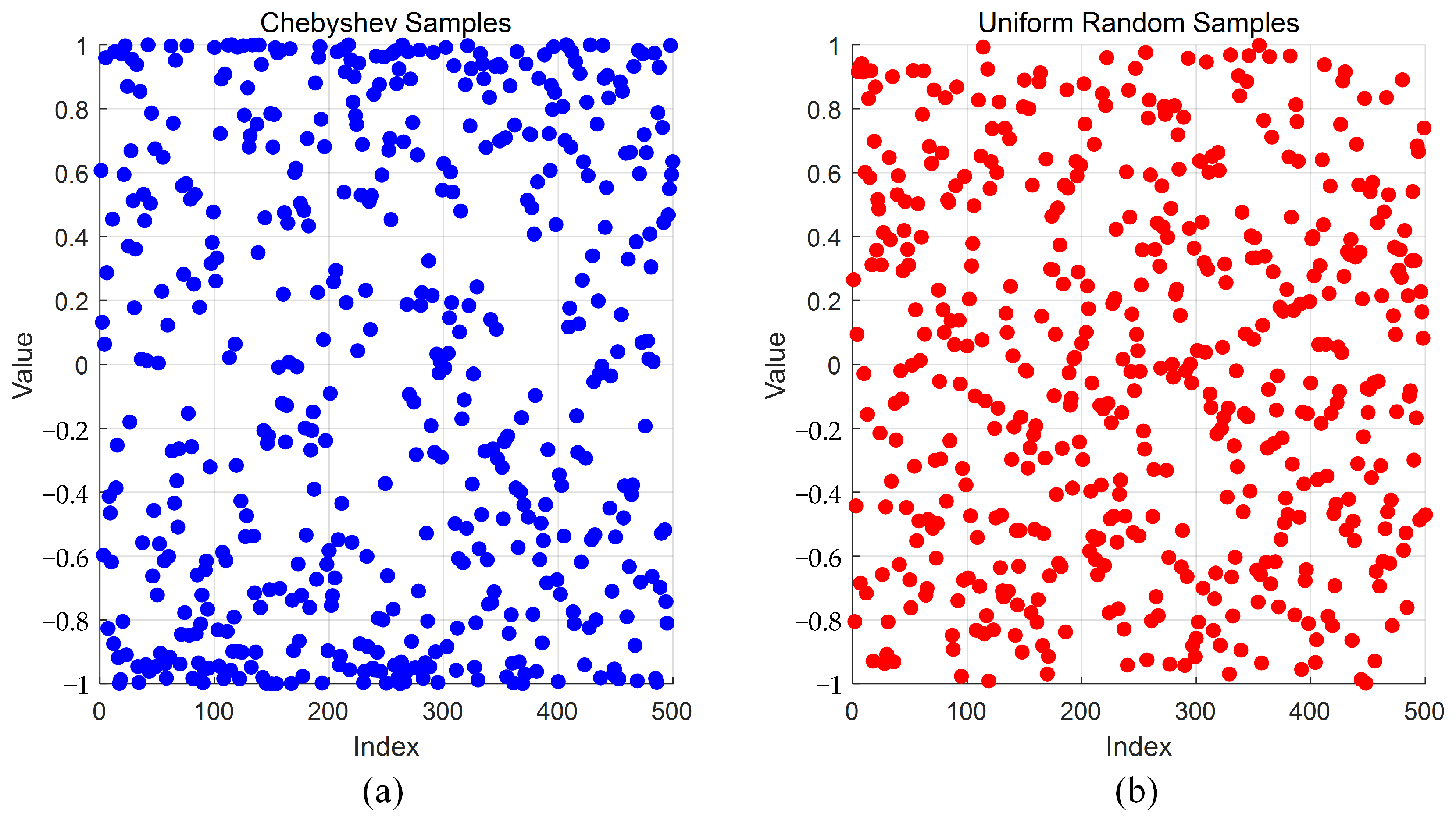
2.3.1. Chebyshev Population Initialization

The inherent randomness in the initial population of both SO and ESO algorithms can lead to inconsistent accuracy and convergence behavior. To enhance the probability of identifying the global optimum, it is beneficial to employ a more uniformly distributed starting configuration. In this work, we leverage the Chebyshev chaotic map to generate the initial snake population. This approach promotes a comprehensive exploration of the solution space, capitalizing on the inherent randomness and ergodicity of chaotic systems [37]. The mathematical representation of the Chebyshev chaotic map is given by Equation (21):

$$X_i(t+1)=cos\left(t{cos}^{-1}\left(X_i\left(t\right)\right)\right)$$

(21)

As shown in Figure 2, while the Chebyshev distribution (Figure 2a) may not appear to be more uniform than random sampling (Figure 2b), it offers significant advantages for optimization. Chebyshev points are strategically concentrated near the boundaries (−1 and 1), where optimal solutions frequently reside in many engineering problems. Additionally, unlike random initialization, Chebyshev sampling provides deterministic and reproducible starting points, enhancing algorithm stability and convergence reliability, especially in complex non-convex landscapes with multiple local optima.

2.3.2. Non-Monotone Temperature Factor

In SO and ESO, the temperature factor influences the behavior of the snake swarm in a monotonic manner. Figure 3 demonstrates that the temperature factor solely depends on the number of iterations, with a threshold value of approximately 220. Before this threshold, the temperature coefficient T consistently remains above 0.6, indicating a “warm” state and foraging activity. Conversely, as the optimization process progresses into its later stages, the temperature shifts to a “cold” state and remains “cold”. This transition indicates that after a significant number of iterations, both SO and ESO are prone to local convergence failure.

To foster an improved equilibrium between localized search and global optimization, a non-monotonic temperature factor is introduced. This is realized through the inclusion of a stochastic parameter, symbolized as a, within the temperature coefficient T at each iteration. By dynamically modulating the temperature in this manner, the algorithm achieves a more efficacious trade-off between exploration and exploitation. Further details regarding the formulation of this adjusted temperature coefficient can be found in Equation (22).

$$T=a\ast {\mathrm{e}}^{-{\displaystyle \frac{t}{t_{max}}}}$$

(22)

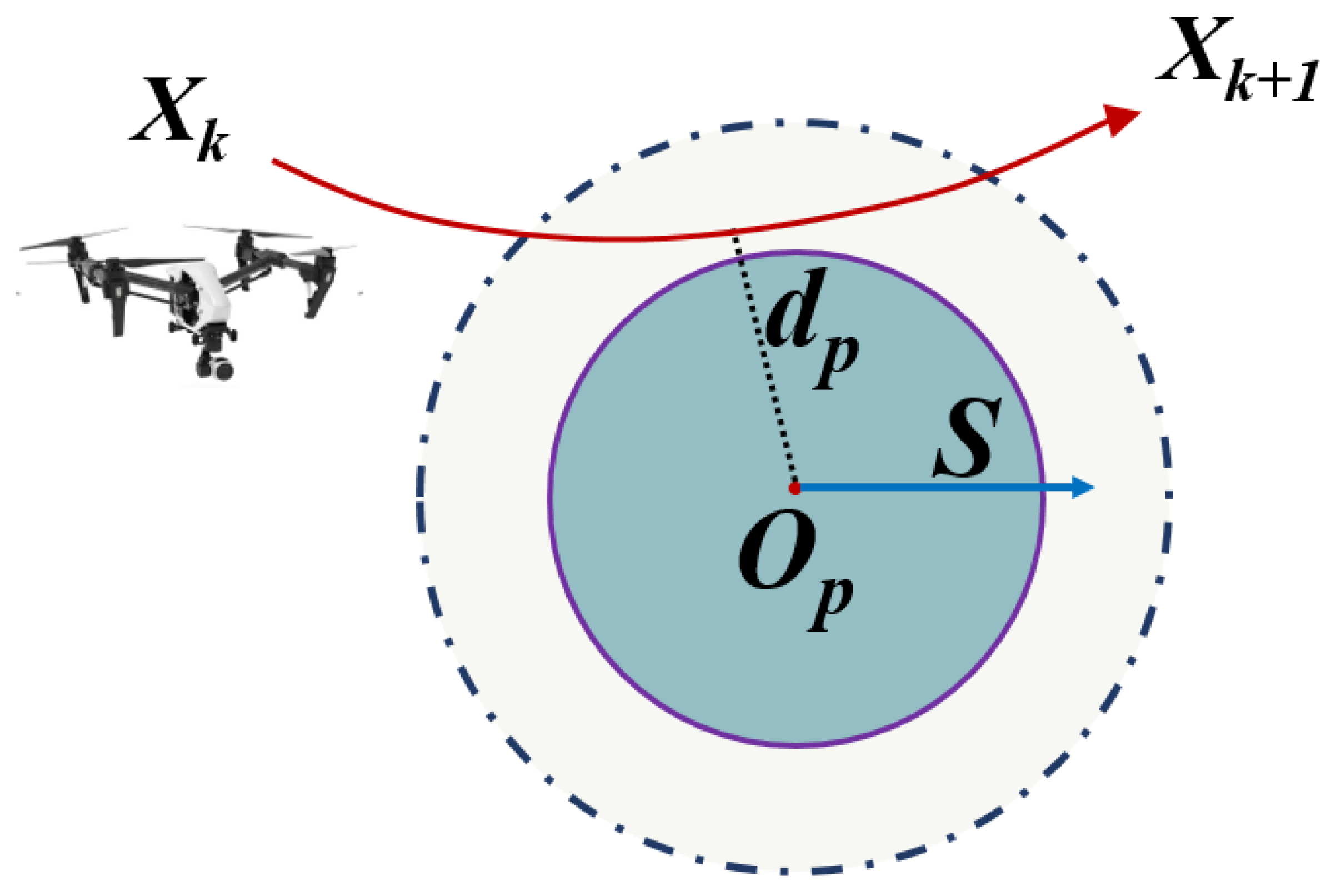
2.3.3. Dynamic-Boundary-Based Opposition Learning (DBOL)

After carefully examining the mirror imaging strategy used in ESO [35] and original opposition-based learning (OBL) [36], it is evident that the ESO mirror method effectively enhances the diversity and quality of the population by calculating the opposition solutions for the current position and then selecting the optimal solution.

However, the performance exhibits a certain degree of uncertainty; while opposition solutions may have greater potential for global optimization, the fixed search upper and lower boundaries limit the ability to estimate the direction of new solutions. We propose a dynamic-boundary-based opposition learning (DBOL) approach to address this issue. DBOL leverages the fact that elite individuals carry more effective information than ordinary ones to refine the opposition process. It fully utilizes the valuable experiences of historical individuals while maintaining a global perspective for new individuals. Through greedy selection, a superior solution is chosen between the current and opposition solutions to participate in the next iteration. The DBOL defines the boundary as follows: Equation (23):

$$X_i^{j^{\ast }}=r_1\left(U{B}_i^j+L{B}_i^j\right)-X_i^j$$

(23)

where $r_1$ is a random value in the interval (0, 1), $U{B}^j=max\left(X_i^j\right)$, $LBj=min\left(X_i^j\right)$, and $U{B}^j$ and $L{B}^j$ are the upper and lower dynamic boundary in the jth dimension, respectively.

2.4. Simulation Experiments Design and the Evaluation Criteria

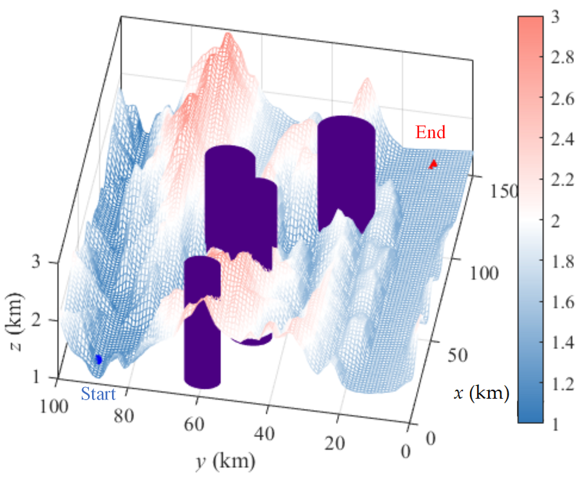
2.4.1. Simulated Experiment

This study’s simulation experiments are divided into two parts: The first part involves selecting the benchmark test functions with a search dimension (D = 30). The objective is to compare different algorithms’ convergence speeds and optimization precision to ascertain whether IESO demonstrates a superior capability to evade local optima when dealing with large-scale optimization problems. The second part entails creating a simulated rugged mountainous terrain to test the path planning. In this experience, the performance of various algorithms is assessed when solving three-dimensional path planning problems based on the three optimization criteria (discussed in Section 2.4.2). It aims to further validate the feasibility of IESO in determining optimal flight paths within intricate, complex landscapes.

We selected thirteen testing functions shown in

Table 1. Formula and parameters of 13 benchmark test functions.

Num.	Name	Formula	Range	${\mathit{f}}_{\mathbf{min}}$
$f_1$	Sphere is Function	$f\left(x\right)={\sum }_{i=1}^n{x}_i^2$	[−100,100]	0
$f_2$	Schwefel’s Problem 2.22	$f\left(x\right)={\sum }_{i=1}^n\left|x_i\right|+{\prod }_{i=1}^n{x}_i$	[−10,10]	0
$f_3$	Schwefel’s Problem 1.2	$f\left(x\right)={\sum }_{i=1}^n{\left({\sum }_{j=1}^i{x}_j\right)}^2$	[−100,100]	0
$f_4$	Schwefel’s Problem 2.21	$f\left(x\right)={max}_i\left\{\left|x_i\right|,1\le i\le n\right\}$	[−100,100]	0
$f_5$	Generalized Rosenbrock’s Function	$f\left(x\right)={\sum }_{i=1}^{n-1}\left[100{\left(x_{i+1}-x_i^2\right)}^2+{\left(x_i-1\right)}^2\right]$	[−30,30]	0
$f_6$	Step Function	$f\left(x\right)={\sum }_{i=1}^d{\left|x_i\right|}^{i+1}$	[−100,100]	0
$f_7$	Quartic Function	$f\left(x\right)={\sum }_{i=1}^{n}i{x}_i^4+\mathrm{random}[0,1]$	[−1.28,1.28]	0
$f_8$	Generalized Schwefel’s Problem 2.26	$f\left(x\right)=418.9829n-{\sum }_{i=1}^n{x}_{i}sin\left(\sqrt{|x_i|}\right)$	[−500,500]	−2094
$f_9$	Generalized Rastrigin’s Function	$f\left(x\right)=10n+{\sum }_{i=1}^n\left(x_i^2-10cos\left(2\pi x_i\right)\right)$	[−10,10]	0
$f_{10}$	Ackley’s Function	$f\left(x\right)=-20exp\left(-0.2\sqrt{{\displaystyle \frac{1}{n}}{\sum }_{i=1}^n{x}_i^2}\right)-exp\left({\displaystyle \frac{1}{n}}{\sum }_{i=1}^{n}cos\left(2\pi x_i\right)\right)+20+e$	[−10,10]	0
$f_{11}$	Generalized Griewank’s Function	$f\left(x\right)=1+{\sum }_{i=1}^n{\displaystyle \frac{x_i^2}{4000}}-{\prod }_{i=1}^{n}cos\left({\displaystyle \frac{x_i}{\sqrt{i}}}\right)$	[−10,10]	0
$f_{12}$	Generalized Penalized Function 1	$f\left(x\right)={\displaystyle \frac{\pi }{n}}\left[10{sin}^2\left(\pi y_1\right)+{\sum }_{i=1}^{n-1}{(y_i-1)}^2\left(1+10{sin}^2\left(\pi y_{i+1}\right)\right)+{(y_n-1)}^2\right]+{\sum }_{i=1}^{n}u(x_i,10,100,4)$	[−10,10]	0
$f_{13}$	Generalized Penalized Function 2	$f\left(x\right)=0.1\left[{sin}^2\left(3\pi x_1\right)+{\sum }_{i=1}^{n-1}{(x_i-1)}^2\left(1+{sin}^2\left(3\pi x_{i+1}\right)\right)+{(x_n-1)}^2\left(1+{sin}^2\left(2\pi x_n\right)\right)\right]+{\sum }_{i=1}^{n}u(x_i,5,100,4)$	[−10,10]	0

.

We selected five algorithms, namely GJO, GWO, HBA, ESO, and SO; their parameters are listed in

Table 2. Algorithm parameters.

Algorithms	Parameters
IESO	$T_{h1}=0.25,T_{h2}=0.6,T_p=50$
ESO	$T_{h1}=0.25,T_{h2}=0.6,c_{start1}=0.5,c_{start2}=0.05,c_{start3}=2;c_{end1}=c_{end2}=c_{end3}=0.5$
SO	$T_{h1}=0.25,T_{h2}=0.6$
GJO	$c_1=1.5,ϵ=1.5$
HBA	$C=2,ϵ=6$
GWO	$a\in [0,2]$

.

We randomly generated the digital elevation model of a simulated rugged mountainous terrain, with map dimensions of 100 km by 150 km by 3 km. The maximum elevation difference is at least 2 km, representing a terrain with significant undulations and numerous ravines. Arbitrary no-fly zones were also added to increase the complexity. Flight waypoints were set to evaluate the effectiveness of the flight paths generated by different algorithms.

The experiments were conducted on a system running the Windows 10 64-bit OS, equipped with an AMD Ryzen 7 4800H processor (AMD, Santa Clara, CA, USA) operating at a frequency of 2.9 GHz, and featuring 16 GB of system memory. The algorithms were implemented and executed using the Matlab2020b software environment.

2.4.2. Evaluation Criteria

Considering the intricate nature of UAV three-dimensional path planning, this study formulates the path planning objective function by incorporating factors such as flight distance, path smoothness, and flight safety. The shortest flight path is defined as shown in Equation (24):

$$F_f=\sum _{k=1}^D\sqrt{{\left(x_{k+1}-x_k\right)}^2+{\left(y_{k+1}-y_k\right)}^2+{\left(z_{k+1}-z_k\right)}^2}$$

(24)

where D represents the number of waypoints and $(x_k,y_k,z_k)$ denotes the coordinates of the kth waypoints. Ensuring smoothness involves minimizing abrupt changes in yaw angle and altitude. Given mountainous areas’ rugged and diverse terrain, flight paths must adhere to maximum climb angles and rates. The path smoothness is given as Equations (25)–(27).

$${\phi }_k=arctan\left({\displaystyle \frac{∥l_k{l}_{k+1}∥}{l_k{l}_{k+1}}}\right)$$

(25)

$${\varphi }_k=arctan\left({\displaystyle \frac{z_{k+1}-z_k}{\sqrt{{\left(x_{k+1}-x_k\right)}^2+{\left(y_{k+1}-y_k\right)}^2}}}\right)$$

(26)

$$F_e=\sum _{k=1}^{D-2}{\phi }_k+\sum _{k=1}^{D-1}\left({\varphi }_k-{\varphi }_{k-1}\right)$$

(27)

where $l_k$ represents the distance between two waypoints. Equations (25) and (26) represent the yaw angle ${\phi }_k$ and pitch angle ${\varphi }_k$, respectively.

A meticulously designed path should prioritize the safe operation of UAVs. The objective function design must incorporate a safety margin, enabling UAVs to avoid obstacles or restricted no-fly zones. As shown in Figure 4 the obstacle within the airspace has a center coordinate of $O_p$ and radius $R_p$. The perpendicular distance $d_p$ from the flight node of the UAV to the obstacle should exceed the safety distance $S_f$, ensuring the UAV operates outside designated shaded regions for safety. The flight safety formula is provided as Equation (28).

$$F_s=\left\{\begin{array}{cc}0,& d_p\ge S\hfill \\ S-d_p,& R_p<d_p<S\hfill \\ \infty ,& d_p<R_p\hfill \end{array}\right.$$

(28)

By integrating these cost functions with weights, an objective function F for the multi-objective path planning problem is formed in Equation (29):

$$F={\omega }_1{F}_f+{\omega }_2{F}_e+{\omega }_3{F}_s$$

(29)

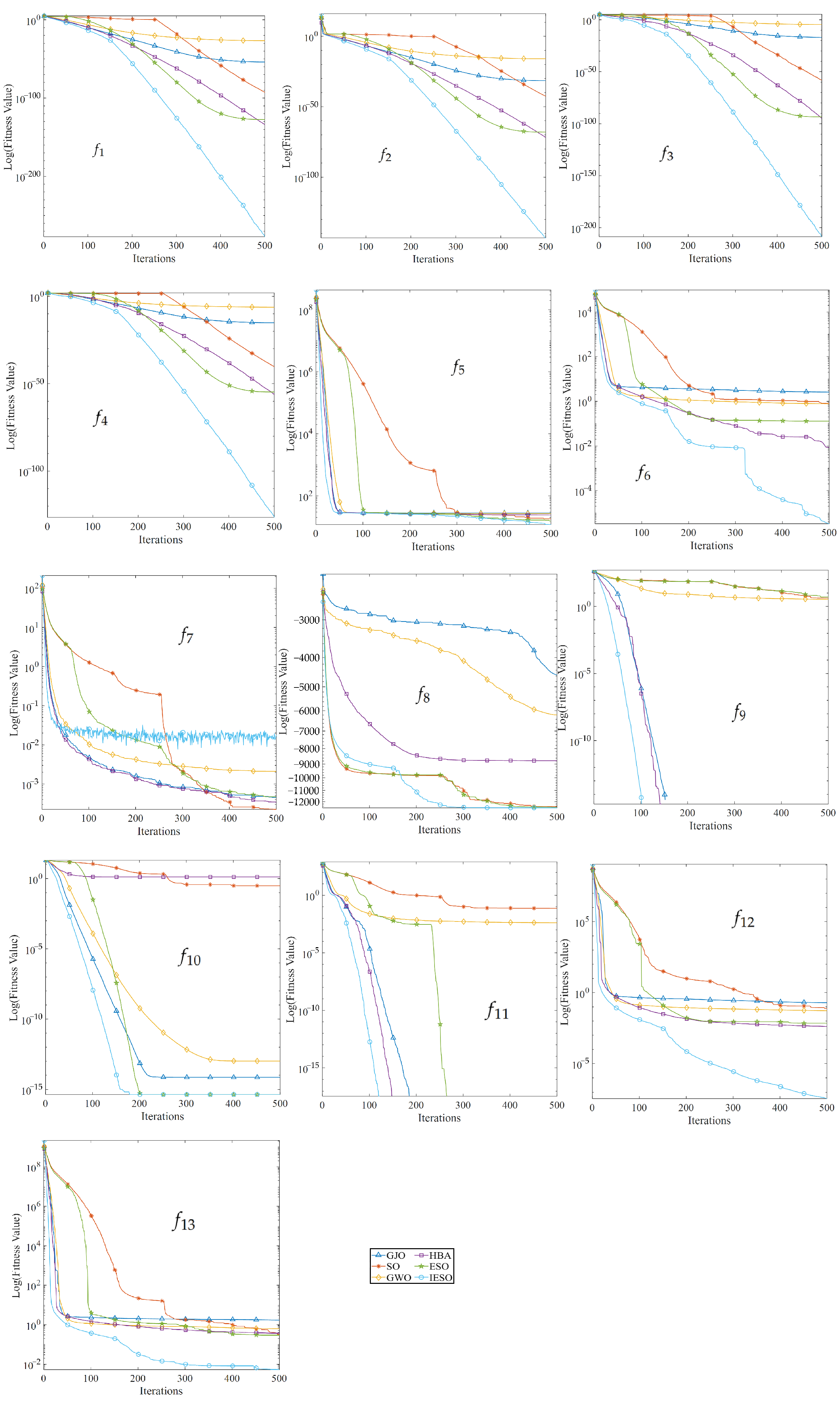
3. Results and Discussion

Table 3. Results obtained from testing with 13 benchmark functions (D = 30) *.

Num.	GJO	SO	GWO	HBA	ESO	IESO
$f_1$	$5.76\times {10}^{-55}$ ($7.15\times {10}^{-55}$)/+	$9.32\times {10}^{-37}$ ($2.69\times {10}^{-36}$)/+	$9.32\times {10}^{-28}$ ($2.82\times {10}^{-28}$)/+	$5.00\times {10}^{-137}$ ($7.43\times {10}^{-137}$)/+	$3.38\times {10}^{-197}$ ($0.00\times {10}^{+00}$)/+	$0.00\times {10}^{-00}$ ($0.00\times {10}^{-00}$)
$f_2$	$1.29\times {10}^{-32}$ ($1.18\times {10}^{-32}$)/+	$6.02\times {10}^{-34}$ ($1.75\times {10}^{-33}$)/+	$6.02\times {10}^{-17}$ ($1.27\times {10}^{-16}$)/+	$4.20\times {10}^{-72}$ ($9.64\times {10}^{-72}$)/+	$5.40\times {10}^{-92}$ ($1.45\times {10}^{-91}$)/+	$7.52\times {10}^{-240}$ ($0.00\times {10}^{-00}$)
$f_3$	$1.37\times {10}^{-17}$ ($2.54\times {10}^{-17}$)/+	$9.89\times {10}^{-17}$ ($1.69\times {10}^{-17}$)/+	$9.89\times {10}^{-06}$ ($6.81\times {10}^{-07}$)/+	$2.81\times {10}^{-101}$ ($4.02\times {10}^{-101}$)/+	$1.10\times {10}^{-150}$ ($2.94\times {10}^{-150}$)/+	$0.00\times {10}^{-00}$ ($0.00\times {10}^{-00}$)
$f_4$	$2.75\times {10}^{-16}$ ($7.85\times {10}^{-16}$)/+	$7.57\times {10}^{-09}$ ($1.25\times {10}^{-08}$)/+	$7.57\times {10}^{-07}$ ($7.28\times {10}^{-07}$)/+	$2.47\times {10}^{-137}$ ($7.43\times {10}^{-137}$)/+	$2.35\times {10}^{-197}$ ($6.41\times {10}^{-77}$)/+	$7.88\times {10}^{-135}$ ($2.94\times {10}^{-134}$)
$f_5$	$2.75\times {10}^{+01}$ ($7.85\times {10}^{-01}$)/+	$7.57\times {10}^{-03}$ ($1.25\times {10}^{-03}$)/+	$2.43\times {10}^{-01}$ ($7.28\times {10}^{-01}$)/+	$2.47\times {10}^{-137}$ ($7.43\times {10}^{-137}$)/+	$2.35\times {10}^{-197}$ ($6.41\times {10}^{-01}$)/+	$1.21\times {10}^{-07}$ ($1.64\times {10}^{-06}$)
$f_6$	$2.76\times {10}^{-04}$ ($3.82\times {10}^{-01}$)/+	$3.10\times {10}^{-05}$ ($5.92\times {10}^{-05}$)/+	$3.10\times {10}^{-28}$ ($2.82\times {10}^{-02}$)/+	$2.56\times {10}^{-137}$ ($7.43\times {10}^{-137}$)/+	$2.79\times {10}^{-197}$ ($7.51\times {10}^{-02}$)/+	$9.52\times {10}^{-08}$ ($1.08\times {10}^{-08}$)
$f_7$	$2.95\times {10}^{-55}$ ($1.66\times {10}^{-04}$)/+	$4.96\times {10}^{-03}$ ($3.33\times {10}^{-04}$)/+	$4.96\times {10}^{-28}$ ($2.82\times {10}^{-04}$)/+	$2.85\times {10}^{-137}$ ($7.43\times {10}^{-137}$)/+	$1.85\times {10}^{-197}$ ($1.88\times {10}^{-04}$)/+	$1.82\times {10}^{-04}$ ($1.03\times {10}^{-04}$)
$f_8$	$-3.70\times {10}^{+03}$ ($1.04\times {10}^{+03}$)/+	$-9.70\times {10}^{+03}$ ($2.27\times {10}^{+03}$)/+	$-9.70\times {10}^{-28}$ ($8.73\times {10}^{+02}$)/+	$-9.02\times {10}^{-137}$ ($7.43\times {10}^{-137}$)/+	$-8.62\times {10}^{+03}$ ($0.00\times {10}^{-00}$)/+	$-1.08\times {10}^{+04}$ ($1.38\times {10}^{+03}$)
$f_9$	$0.00\times {10}^{-00}$ ($0.00\times {10}^{-00}$)/=	$0.00\times {10}^{-00}$ ($0.00\times {10}^{-00}$)/=	$2.18\times {10}^{-02}$ ($5.68\times {10}^{-14}$)/+	$0.00\times {10}^{-00}$ ($0.00\times {10}^{-00}$)/=	$0.00\times {10}^{-00}$ ($0.00\times {10}^{-00}$)/=	$0.00\times {10}^{-00}$ ($0.00\times {10}^{-00}$)
$f_{10}$	$6.13\times {10}^{-55}$ ($1.83\times {10}^{-15}$)/+	$1.87\times {10}^{-15}$ ($2.48\times {10}^{-15}$)/+	$1.86\times {10}^{-13}$ ($1.48\times {10}^{-14}$)/+	$8.88\times {10}^{-00}$ ($0.00\times {10}^{-00}$)/=	$8.88\times {10}^{-16}$ ($0.00\times {10}^{-00}$)/=	$8.88\times {10}^{-16}$ ($0.00\times {10}^{-00}$)
$f_{11}$	$0.00\times {10}^{-00}$ ($0.00\times {10}^{-00}$)/=	$0.00\times {10}^{-00}$ ($0.00\times {10}^{-00}$)/=	$0.00\times {10}^{-00}$ ($0.00\times {10}^{-00}$)/=	$0.00\times {10}^{-00}$ ($0.00\times {10}^{-00}$)/=	$0.00\times {10}^{-00}$ ($0.00\times {10}^{-00}$)/=	$0.00\times {10}^{-00}$ ($0.00\times {10}^{-00}$)
$f_{12}$	$2.95\times {10}^{-02}$ ($1.66\times {10}^{-02}$)/+	$4.96\times {10}^{-07}$ ($3.33\times {10}^{-07}$)/+	$4.96\times {10}^{-02}$ ($7.30\times {10}^{-02}$)/+	$2.85\times {10}^{-04}$ ($1.78\times {10}^{-03}$)/+	$1.85\times {10}^{-09}$ ($5.88\times {10}^{-09}$)/=	$2.53\times {10}^{-09}$ ($3.26\times {10}^{-09}$)
$f_{13}$	$1.75\times {10}^{-00}$ ($2.20\times {10}^{-01}$)/+	$2.98\times {10}^{-05}$ ($8.17\times {10}^{-05}$)/+	$2.95\times {10}^{-05}$ ($1.74\times {10}^{-01}$)/+	$3.80\times {10}^{-01}$ ($2.76\times {10}^{-01}$)/+	$1.43\times {10}^{-01}$ ($1.72\times {10}^{-01}$)/+	$7.13\times {10}^{-08}$ ($7.36\times {10}^{-08}$)
Wilcoxon Test Summary $+/=/-$	12/1/0	10/3/0	12/1/0	9/4/0	8/5/0	Wilcoxon

* The data format: average/standard deviation/Wilcoxon test sign (+/−/=).

summarizes the test results across six algorithms. The lowest average optimization result for each test function is highlighted, indicating superior performance. Statistical significance was assessed using the rank-sum test, where “+”, “−”, and “=” denote that the Improved Enhanced Snake Optimizer (IESO) performs better than, worse than, or equivalent to other algorithms, respectively.

The statistical analysis demonstrates that IESO generally outperforms the majority of tested algorithms. Integrating multiple strategies significantly improves both the convergence precision and stability of IESO compared to the standard Snake Optimizer (SO), providing preliminary confirmation of the effectiveness of these enhancements. Figure 5 illustrates the convergence curves of the objective function value (fitness) versus the number of iterations for all compared algorithms. The vertical axis denotes the logarithm of the best-so-far objective value. Note that some functions can reach extremely small values (e.g., below 10–200), which is due to the nature of the benchmark functions and high optimization precision of the algorithms. Figure 5 shows that, for any given test benchmark function with D = 30, only one algorithm outperforms IESO.

The Improved Enhanced Snake Optimizer (IESO) demonstrates exceptional performance across thirteen test functions. This superior performance stems from a innovative approach involving a non-monotonic temperature factor that strategically enhances interactions between different search modes. By leveraging the global best position, the algorithm’s foraging mode generates high-quality solutions, significantly accelerating convergence and improving overall optimization efficiency. The nuanced temperature factor management enables more dynamic and adaptive search strategies, distinguishing IESO from conventional optimization approaches.

The only exception is $f_{12}$, where ESO slightly outperforms our IESO. The algorithm sometimes encounters local optima due to their abundance, posing a challenge for global optimization; while the mirroring mechanism expands exploration, limited executions and narrowing boundaries can still trap the optimizer. To address this, incorporating Lévy flights, with their varying step lengths, is suggested to help the algorithm escape local optima, as previously proposed by Wang et al. [38]. In our IESO, we employed a dynamic boundary to the opposite learning mechanism to enhance performance further, which has better results escaping the local optima than ESO. However, in some cases, it may not be fully utilized.

A simulated digital elevation model of rugged mountainous terrain was obtained, with the map dimensions measuring 100 km by 150 km by 3 km. The maximum elevation difference in this area exceeds 2 km, featuring a terrain with significant undulations and numerous ravines. Randomly generated “no-fly zones” within this terrain are added and are illustrated in Figure 6 (purple areas). The launch point is set at coordinates (10, 90, 1.115), and the destination is at (130, 10, 1.373), with all units in kilometers (km). The fundamental challenge of path planning lies in identifying suitable waypoints during the flight to achieve an optimal flight route. To this end, this study sets 15 flight waypoints within the three-dimensional map and then employs interpolation to obtain detailed flight paths between adjacent waypoints. The parameters to be optimized are the spatial coordinates of these 15 waypoints.

The six algorithms, ESO, SO, GJO, HBA, GWO and our IESO, were selected to plan the optimized routing on this simulated terrain. We conducted over a hundred simulation runs. From

Table 4. Algorithm performance statistics (path length).

Algorithms	Best	Average	Worst	Standard	Difference
IESO	78.944	78.990	80.332	0.253	-
ESO	120.260	120.260	120.260	$2.89\times {10}^{-14}$	+34.32
SO	123.640	123.76	123.760	0.022	+36.17
GJO	89.466	89.466	89.466	$7.22\times {10}^{-14}$	+11.71
HBA	113.730	113.730	113.730	$4.33\times {10}^{-14}$	+30.54
GWO	123.760	123.870	123.87	$7.22\times {10}^{-14}$	+36.23

, we can see that the IESO clearly outperforms the other algorithms from 11.71 (GJO) to 36.25% (SO). One sample run was shown in Figure 7, where IESO exhibits a significantly faster convergence time than the other algorithms, at least 20% faster than GJO and over 35% faster than ESO. Additionally, Figure 8 and Figure 9 demonstrate that one sample of the route proposed by IESO is the shortest and successfully avoids all no-fly zones, as seen from both 2D and 3D perspectives. It is at least 10% shorter than the competitors. Therefore, we can conclusively state that IESO significantly improves flight planning in complex environments, such as rugged mountain terrains with substantial undulations and numerous ravines, while effectively avoiding arbitrary no-fly zones.

4. Conclusions

This study introduces the Improved Enhanced Snake Optimizer (IESO) as a novel approach to optimizing 3D UAV path planning in challenging environments, such as rugged mountainous terrains. By integrating Chebyshev chaotic mapping, a non-monotonically decreasing temperature factor, and dynamic-boundary-based opposition learning (DBOL), the IESO enhances exploration capabilities. It also improves exploitation capabilities, leading to more efficient path solutions.

To validate its effectiveness, we conducted extensive simulations using thirteen benchmark test functions, comparing the IESO against five state-of-the-art optimization algorithms. The results consistently demonstrated the superiority of IESO, achieving over 30% shorter path distances and a 10% improvement in computational efficiency. These improvements highlight the algorithm’s potential for real-world UAV applications where precise and efficient navigation is crucial.

Future research could focus on further refining the algorithm through adaptive parameter tuning and the integration of real-time environmental feedback. Moreover, evaluating IESO in actual UAV flight scenarios would offer valuable insights into its practical applicability and robustness under dynamic conditions. Currently, the evaluation is limited to simulations, with no testing on real-world data or incorporation of real-time or dynamic obstacle avoidance. Addressing these limitations in future work will enhance IESO’s potential as a powerful tool for autonomous UAV operations in complex terrains.

References

1. Zhang, W.; Li, J.; Yu, W.; Ding, P.; Wang, J.; Zhang, X. Algorithm for UAV path planning in high obstacle density environments: RFA-star. Front. Plant Sci. 2024, 15, 1391628. [Google Scholar] [CrossRef] [PubMed]
2. Jones, M.; Djahel, S.; Welsh, K. Path-Planning for Unmanned Aerial Vehicles with Environment Complexity Considerations: A Survey. ACM Comput. Surv. 2023, 55, 1–39. [Google Scholar] [CrossRef]
3. Aggarwal, S.; Kumar, N. Path planning techniques for unmanned aerial vehicles: A review, solutions, and challenges. Comput. Commun. 2020, 149, 270–299. [Google Scholar] [CrossRef]
4. Yahia, H.S.; Mohammed, A.S. Path Planning Optimization in Unmanned Aerial Vehicles Using Metaheuristic Algorithms: A systematic review. Environ. Monit. Assess. 2023, 195, 30. [Google Scholar] [CrossRef]
5. Li, D.; Yin, W.; Wong, W.E.; Jian, M.; Chau, M. Quality-oriented Hybrid Path Planning Based on A* and Q-learning for Unmanned Aerial Vehicle. IEEE Access 2021, 10, 7664–7674. [Google Scholar] [CrossRef]
6. Pan, Z.; Zhang, C.; Xia, Y.; Xiong, H.; Shao, X. An Improved Artificial Potential Field Method for Path Planning and Formation Control of the Multi-UAV Systems. IEEE Trans. Circuits Syst. II Express Briefs 2022, 69, 1129–1133. [Google Scholar] [CrossRef]
7. Wang, J.; Li, Y.; Li, R.; Chen, H.; Chu, K. Trajectory Planning for UAV Navigation in Dynamic Environments with Matrix Alignment Dijkstra. Appl. Soft Comput. 2022, 26, 12599–12610. [Google Scholar] [CrossRef]
8. Prasad, N.L.; Ramkumar, B. 3-D Deployment and Trajectory Planning for Relay Based UAV Assisted Cooperative Communication for Emergency Scenarios Using Dijkstra’s Algorithm. IEEE Trans. Veh. Technol. 2022, 72, 5049–5063. [Google Scholar] [CrossRef]
9. Flores-Caballero, G.; Rodríguez-Molina, A.; Aldape-Pérez, M.; Villarreal-Cervantes, M.G. Optimized Path-Planning in Continuous Spaces for Unmanned Aerial Vehicles Using Meta-Heuristics. IEEE Access 2020, 8, 176774–176788. [Google Scholar] [CrossRef]
10. Lin, H.; Liu, T. Research on path planning method of driverless vehicle based on improved A* algorithm. J. Hunan Univ. Arts Sci. 2021, 33, 17–20. [Google Scholar]
11. He, Y.; Hou, T.; Wang, M. A new method for unmanned aerial vehicle path planning in complex environments. Sci. Rep. 2024, 14, 9257. [Google Scholar] [CrossRef] [PubMed]
12. Shao, S.; He, C.; Zhao, Y.; Wu, X. Efficient Trajectory Planning for UAVs Using Hierarchical Optimization. IEEE Access 2021, 9, 60668–60681. [Google Scholar] [CrossRef]
13. Chen, J.C.; Ling, F.Y.; Zhang, Y.; You, T.; Liu, Y.F.; Du, X.Y. Coverage Path Planning of Heterogeneous Unmanned Aerial Vehicles Based on Ant Colony System. Swarm Evol. Comput. 2022, 69, 101005. [Google Scholar] [CrossRef]
14. Fu, J.; Sun, G.; Liu, J.; Yao, W.; Wu, L. On Hierarchical Multi-UAV Dubins Traveling Salesman Problem Paths in a Complex Obstacle Environment. IEEE Trans. Cybern. 2024, 4, 3265926. [Google Scholar] [CrossRef]
15. Fu, J.; Yao, W.; Sun, G.; Ma, Z.; Dong, B.; Ding, J. Multirobot Cooperative Path Optimization Approach for Multiobjective Coverage in a Congestion Risk Environment. IEEE Trans. Syst. Man Cybern. Syst. 2024, 54, 1816–1827. [Google Scholar] [CrossRef]
16. Zhao, F.; Li, D.; Wang, Z.; Mao, J.; Wang, N. Autonomous localized path planning algorithm for UAVs based on TD3 strategy. Sci. Rep. 2024, 14, 763. [Google Scholar] [CrossRef]
17. Luo, J.; Tian, Y.; Wang, Z. Research on Unmanned Aerial Vehicle Path Planning. Drone 2024, 8, 51. [Google Scholar] [CrossRef]
18. Wang, H.; Pan, W. Research on UAV Path Planning Algorithms. IOP Conf. Ser. Earth Environ. Sci. 2021, 693, 012120. [Google Scholar] [CrossRef]
19. Debnath, D.; Vanegas, F.; Sandino, J.; Hawary, A.F.; Gonzalez, F. A Review of UAV Path-Planning Algorithms and Obstacle Avoidance Methods for Remote Sensing Applications. Remote Sens. 2024, 16, 4019. [Google Scholar] [CrossRef]
20. Yao, L.; Yuan, P.; Tsai, C.Y.; Zhang, T.; Lu, Y.; Ding, S. ESO: An Enhanced Snake Optimizer for Real-world Engineering Problems. Expert Syst. Appl. 2023, 230, 120594. [Google Scholar] [CrossRef]
21. Hashim, F.A.; Hussien, A.G. Snake Optimizer: A Novel Meta-heuristic Optimization Algorithm. Expert Syst. Appl. 2022, 242, 108320. [Google Scholar] [CrossRef]
22. Wolpert, D.H.; Macready, W.G. No Free Lunch Theorems for Optimization. IEEE Trans. Evol. Comput. 1997, 1, 67–82. [Google Scholar] [CrossRef]
23. Chopra, N.; Ansari, M.M. Golden Jackal Optimization: A Novel Nature-inspired Optimizer for Engineering Applications. Expert Syst. Appl. 2022, 198, 116924. [Google Scholar] [CrossRef]
24. Mirjalili, S.; Mirjalili, S.M.; Lewis, A. Grey Wolf Optimizer. Adv. Eng. Softw. 2014, 69, 46–61. [Google Scholar] [CrossRef]
25. Hashim, F.A.; Houssein, E.H.; Hussain, K.; Mabrouk, M.S.; Al-Atabany, W. Honey Badger Algorithm: New Metaheuristic Algorithm for Solving Optimization Problems. Math. Comput. Simul. 2022, 192, 84–110. [Google Scholar] [CrossRef]
26. Nadimi-Shahraki, M.; Taghian, S.; Mirjalili, S. An Improved Grey Wolf Optimizer for Solving Engineering Problems. Expert Syst. Appl. 2021, 166, 113917. [Google Scholar] [CrossRef]
27. Qi, D.; Chan, W.H.; Zain, A.M.; Junaidi, A.; Yang, H. An improved algorithm based on snake optimizer. Proc. Comput. Sci. 2023, 1, 0017. [Google Scholar] [CrossRef]
28. Mai, C.; Zhang, L.; Hu, X. An adaptive snake optimization algorithm incorporating Subtraction-Average-Based Optimizer for photovoltaic cell parameter identification. Heliyon 2024, 10, 15. [Google Scholar] [CrossRef]
29. Zheng, W.; Ai, Y.; Zhang, W. Improved Snake Optimizer Using Sobol Sequential Nonlinear Factors and Different Learning Strategies and Its Applications. Mathematics 2024, 12, 1708. [Google Scholar] [CrossRef]
30. Li, S.; Tang, Z. An Enhanced Snake Optimizer Algorithm for Feature Selection. In Proceedings of the 2023 8th International Conference on Big Data and Computing, Shenzhen, China, 26–28 May 2023; pp. 81–86. [Google Scholar] [CrossRef]
31. Zhu, Y.; Huang, H.; Wei, J.; Yi, J.; Liu, J.; Li, M. ISO: An improved snake optimizer with multi-strategy enhancement for engineering optimization. Expert Syst. Appl. 2025, 281, 127660. [Google Scholar] [CrossRef]
32. Zhang, J.; Zhang, G.; Kong, M.; Zhang, T.; Wang, D. CGJO: A novel complex-valued encoding golden jackal optimization. Sci. Rep. 2024, 14, 19577. [Google Scholar] [CrossRef] [PubMed]
33. Hassan, I.H.; Abdullahi, M.; Isuwa, J.; Yusuf, S.A.; Aliyu, I.T. A comprehensive survey of honey badger optimization algorithm and meta-analysis of its variants and applications. Frankl. Open 2024, 8, 100141. [Google Scholar] [CrossRef]
34. Jiang, J.; Zhao, Z.; Li, W.; Li, K. An Enhanced Grey Wolf Optimizer with Elite Inheritance and Balance Search Mechanisms. arXiv 2024. [Google Scholar] [CrossRef]
35. Xu, Y.; Li, X.; Yang, J.; Zhang, D. Integrate the original face image and its mirror image for face recognition. Neurocomputing 2014, 131, 191–199. [Google Scholar] [CrossRef]
36. Tizhoosh, H.R. Opposition-based learning: A new scheme for machine intelligence. In Proceedings of the International Conference on Computational Intelligence for Modelling, Control and Automation and International Conference on Intelligent Agents, Web Technologies and Internet Commerce (CIMCA-IAWTIC’06), Vienna, Austria, 28–30 November 2005; Volume 131, pp. 695–701. [Google Scholar] [CrossRef]
37. Wu, T.Y.; Li, H.; Chu, S.C. CPPE: An Improved Phasmatodea Population Evolution Algorithm with Chaotic Maps. Mathematics 2023, 11, 1977. [Google Scholar] [CrossRef]
38. Wang, C.; Jiao, S.; Li, Y.; Zhang, Q. Capacity Optimization of a Hybrid Energy Storage System Considering Wind-Solar Reliability Evaluation Based on A Novel Multi-strategy Snake Optimization Algorithm. Expert Syst. Appl. 2023, 231, 120602. [Google Scholar] [CrossRef]
Figure 1. IESO flowchart.
Wevj 16 00295 g001
Figure 2. Initial value distribution using the (a) Chebyeshev chaotic map and (b) normal random distribution.
Wevj 16 00295 g002
Figure 3. Temperature factor.
Wevj 16 00295 g003
Figure 4. Flight safety to avoid obstacles or restricted no-fly zones.
Wevj 16 00295 g004
Figure 5. Convergence curves of the optimization algorithms on 13 benchmark functions.
Wevj 16 00295 g005
Figure 6. The sample of a simulated rugged mountain terrain with “no-fly” zones.
Wevj 16 00295 g006
Figure 7. One sample of the iteration fitness curves for the six algorithms.
Wevj 16 00295 g007
Figure 8. One sample of the planned routes from the six algorithms.
Wevj 16 00295 g008
Figure 9. One sample of the IESO planned route on the simulated terrain.
Wevj 16 00295 g009