
Smart Monitoring of Microgrid-Integrated Renewable-Energy-Powered Electric Vehicle Charging Stations Using Synchrophasor Technology


Abstract
1. Introduction
- (i)
- Investigating both hybrid stand-alone and grid-connected systems and analyzing them from technical, economic, and environmental perspectives;
- (ii)
- Comparing various system setups and recommending the most suitable sizes for different hybrid components;
- (iii)
- Examining the incorporation of PV–Wind and PV-only systems that satisfy similar load demands on the grid, and contrasting them with standalone Hybrid Energy Systems (HESs);
- (iv)
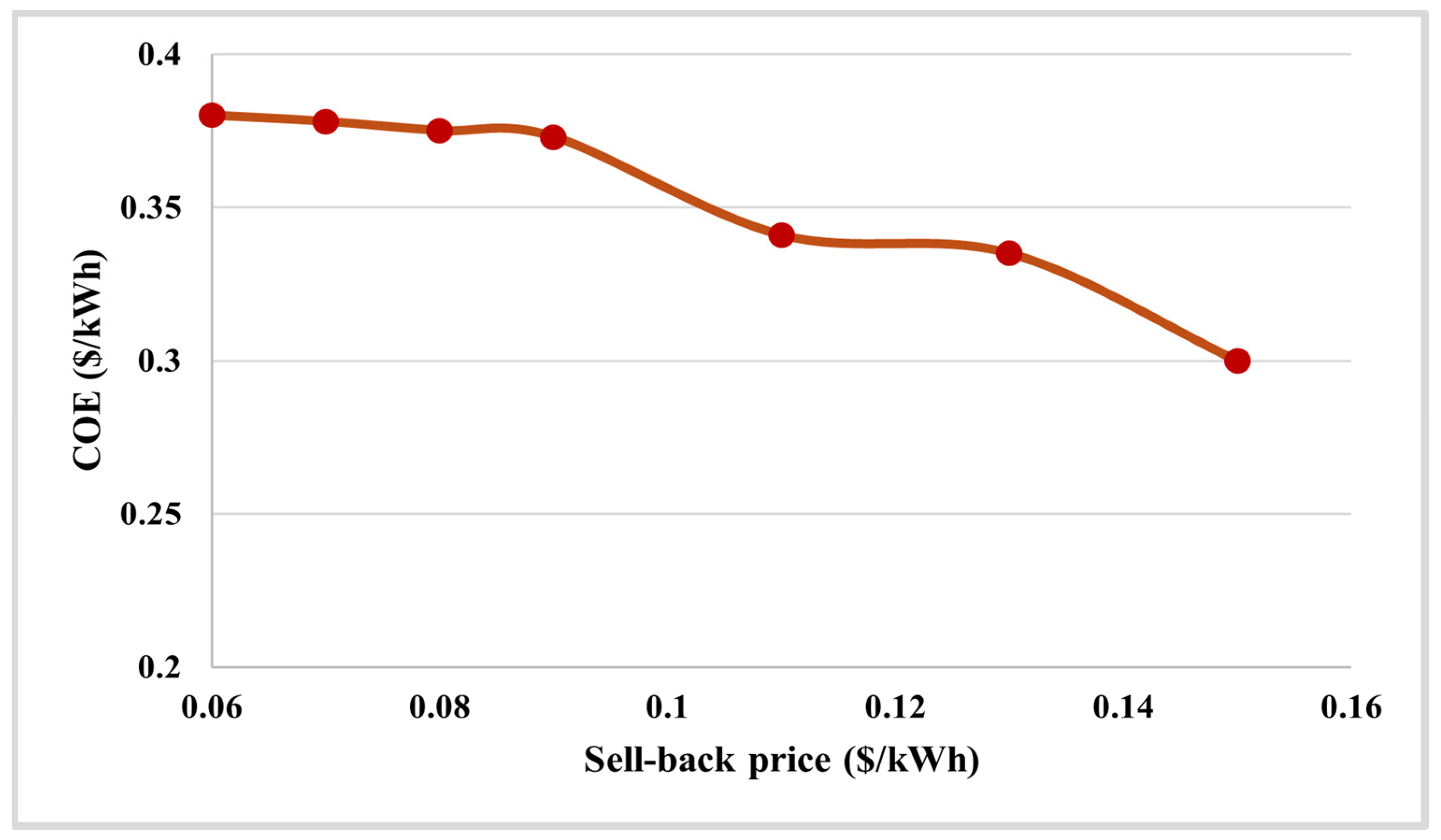
- Analyzing how the cost of energy (COE) is affected by grid sell-back prices;
- (v)
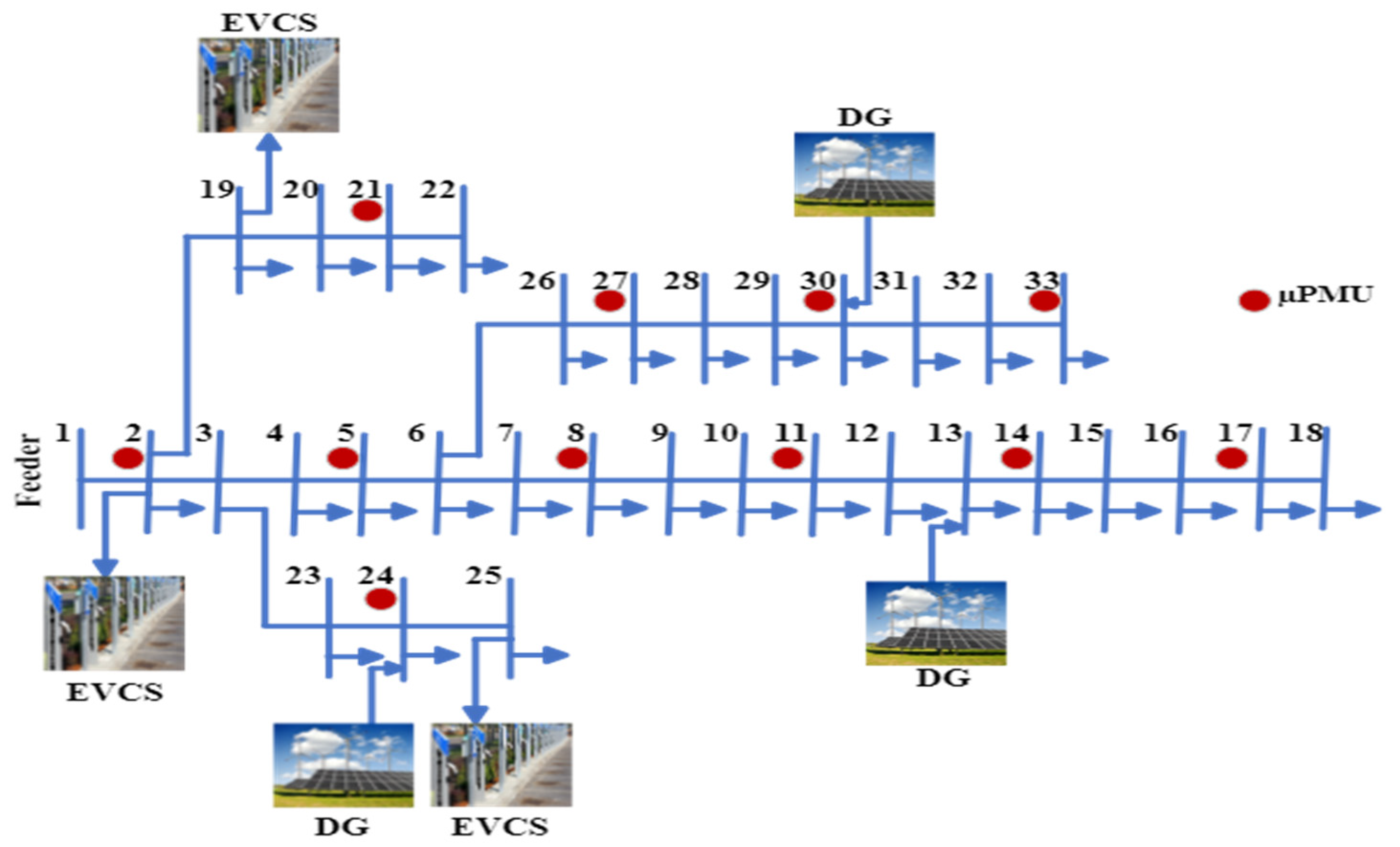
- Conducting an analysis of the IEEE 33 bus architecture using micro-pmu (µPMU) with Electric Vehicle Charging Stations (EVCS) and Distributed Generators (DGs).
2. Materials and Methods
2.1. Mathematical Modeling
2.1.1. PV–Wind Module
2.1.2. Converter
2.1.3. Battery
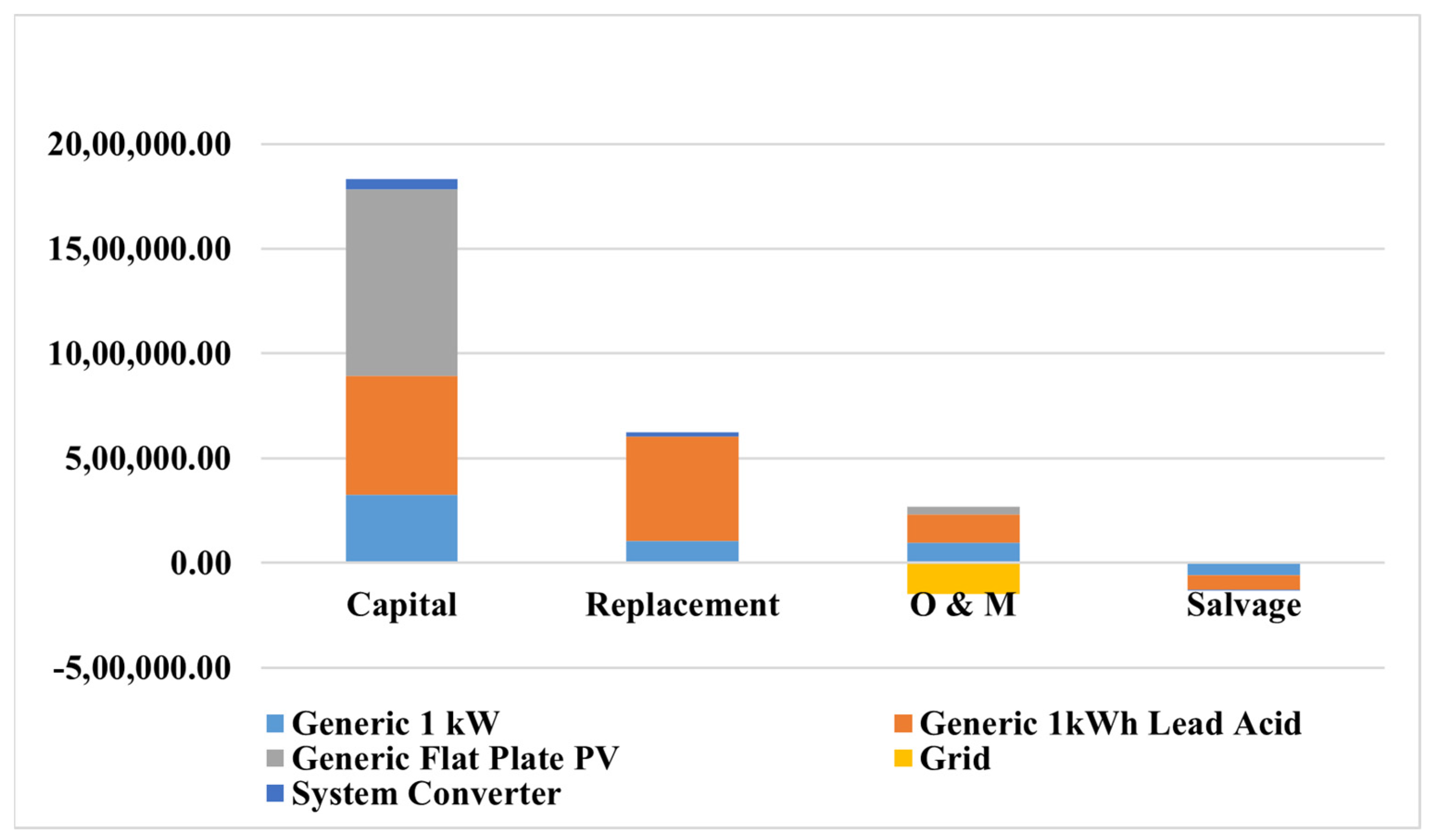
2.1.4. Financial Components
- (a)
- Cost of Energy
- (b)
- Net Present Value
2.1.5. CO2 Emissions
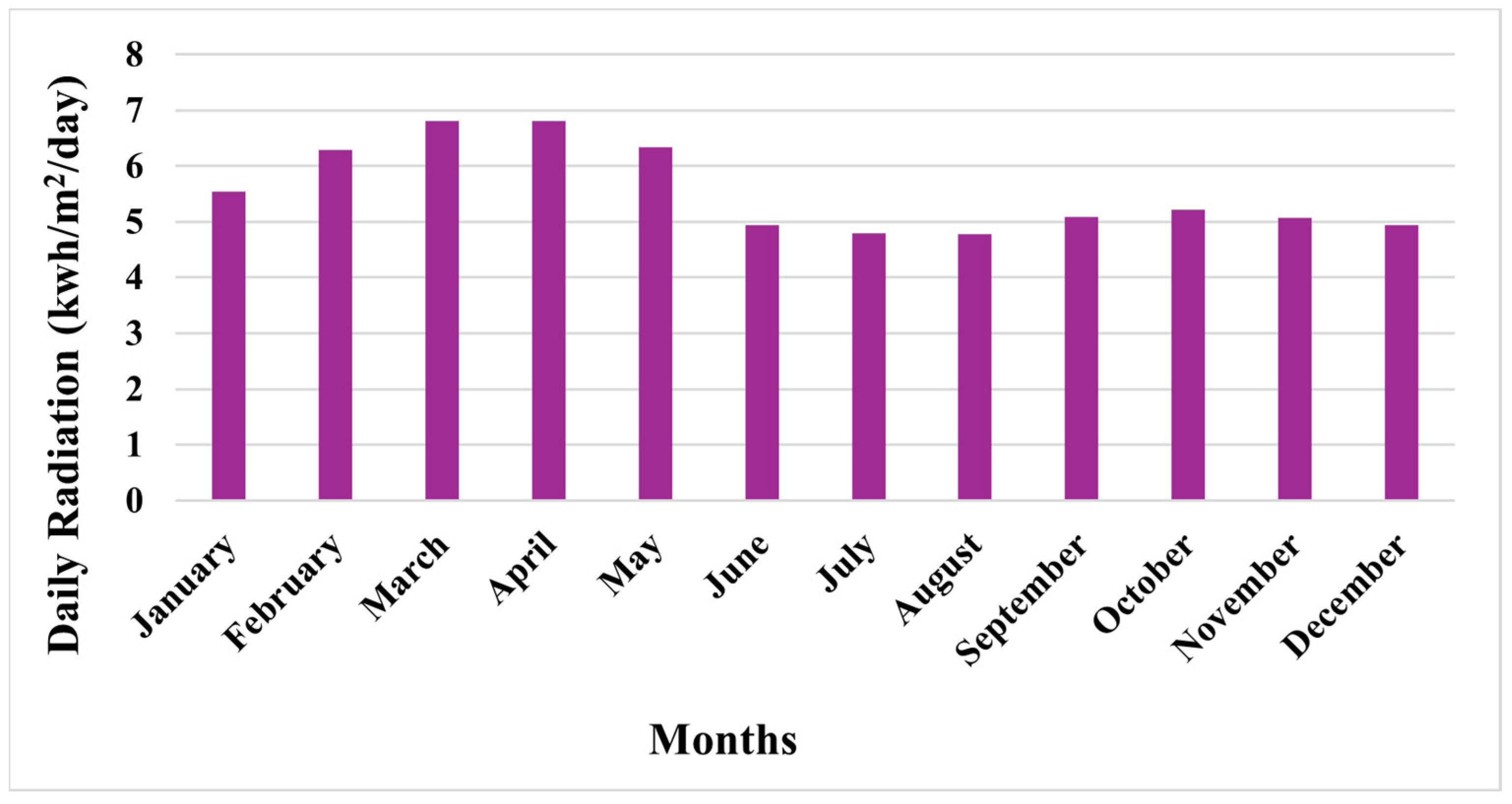
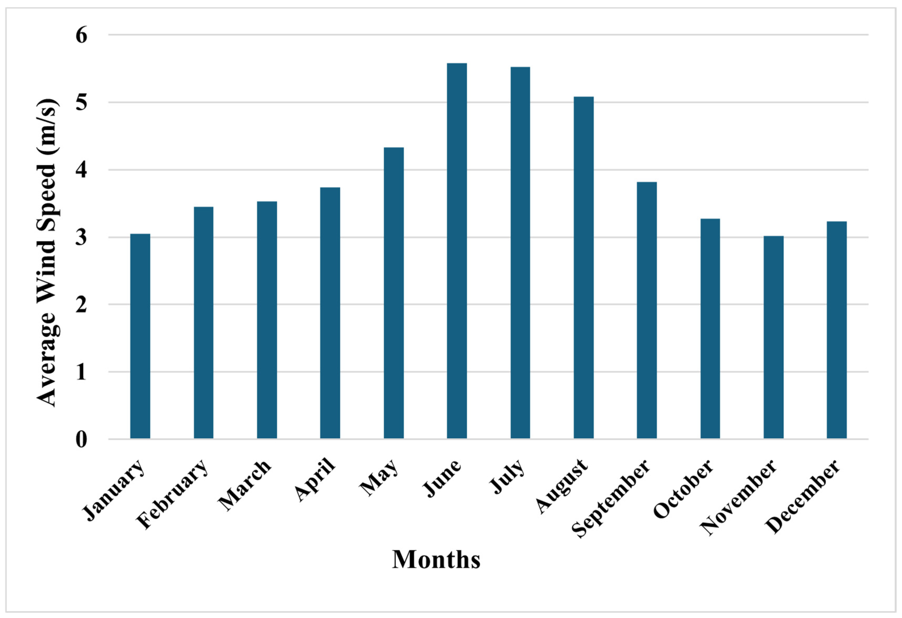
2.2. Selected Site Description
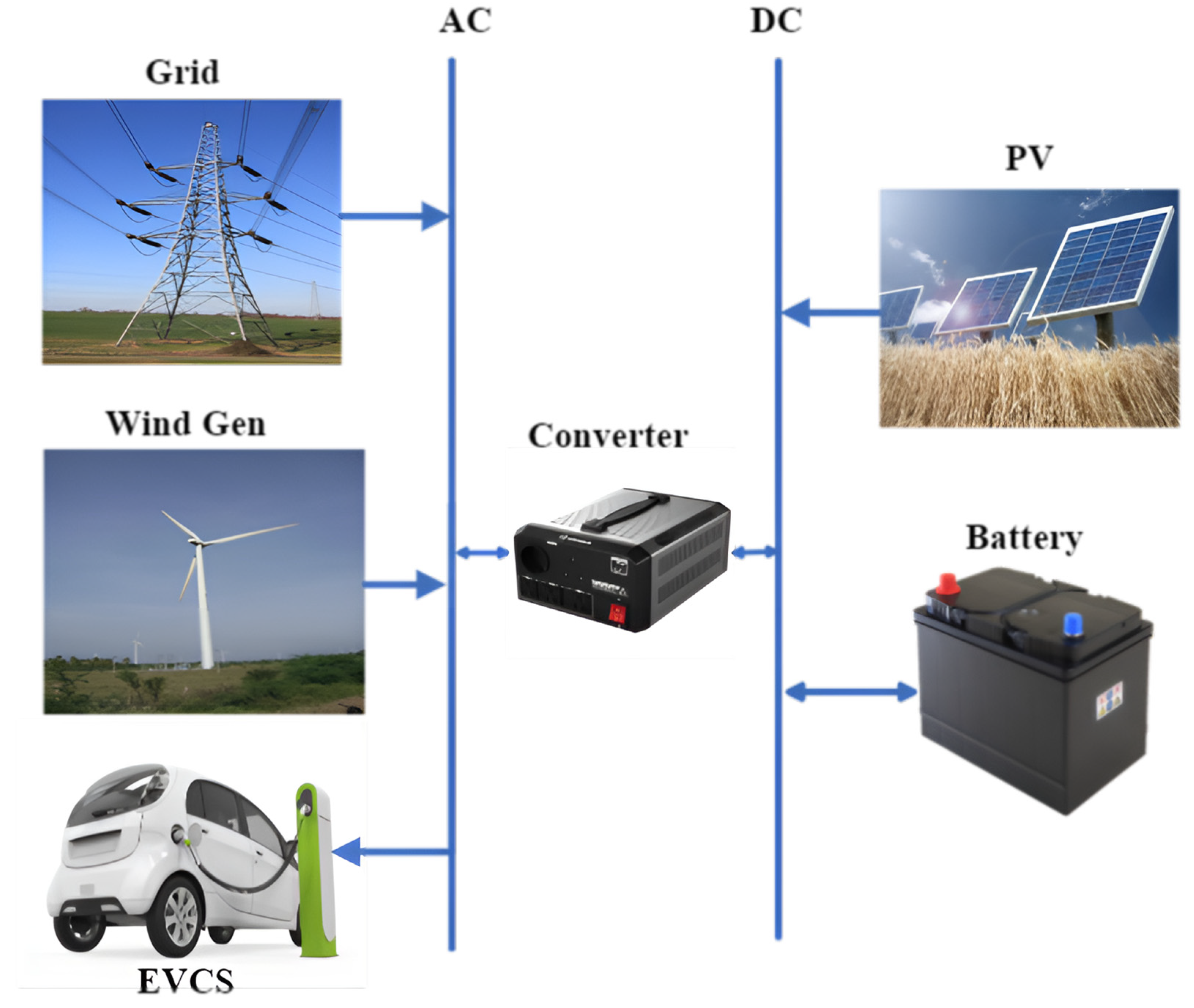
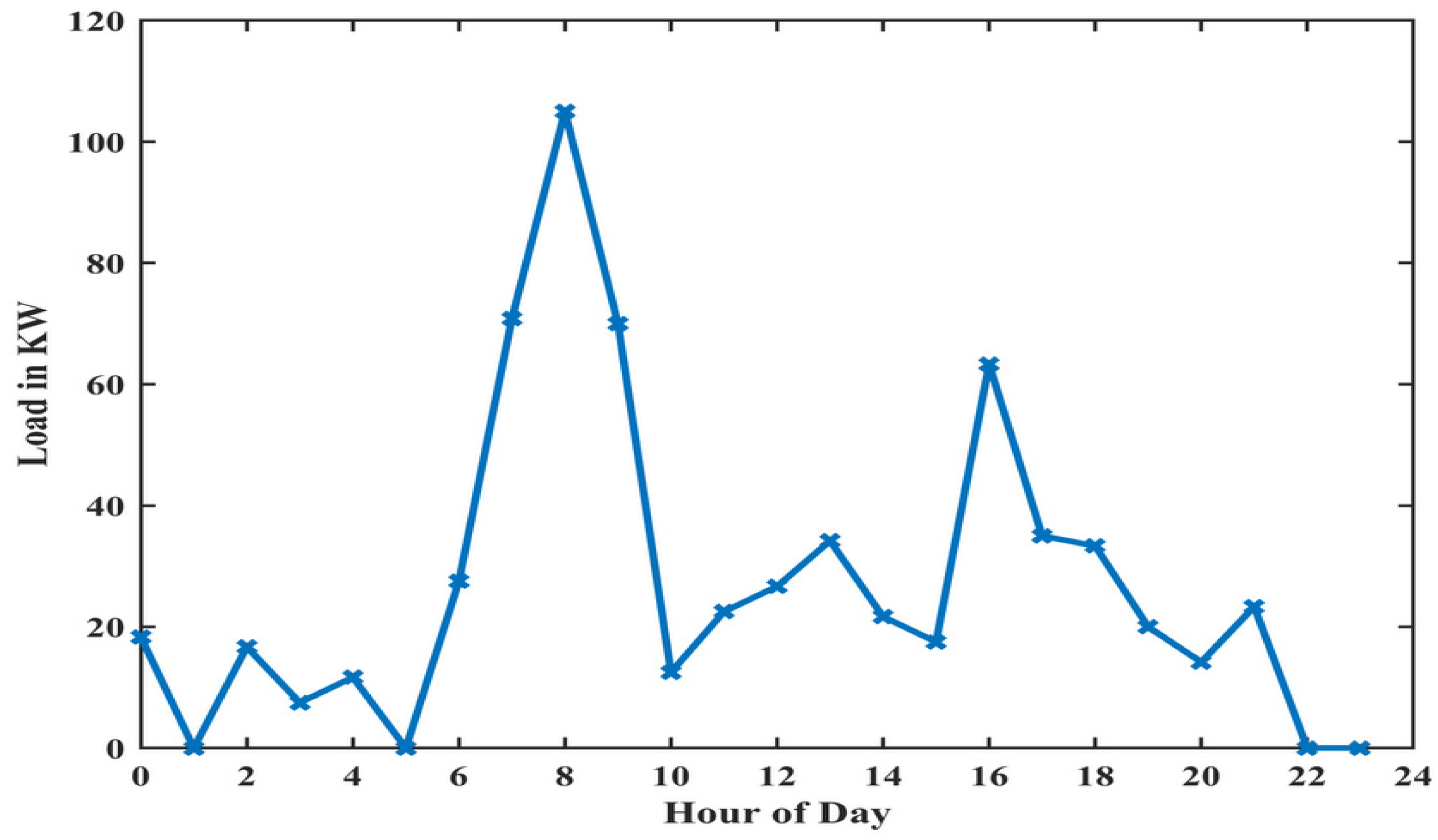
2.3. System Description
3. Results and Discussion

| Component | Size | Capital Cost ($/kW) | Replacement Cost ($/kW) | O&M Cost ($/kW) | Lifetime | Other Parameters |
|---|---|---|---|---|---|---|
| PV | 300 kW 200 kW | 3000 | 2500 | 100 | 25 years | Derating factor, 88% |
| Wind | 167 kW 109 kW | 3000 | 3000 | 70 | 20 years | Hub height, 17 m |
| Converter | 118 kW 126 kW 120 kW 158 kW | 300 | 300 | -- | 15 years | Converter efficiency, 98% Rectifier efficiency, 95% |
| Battery | 3122 kWh 1607 kWh 1710 kWh 1029 kWh | 550 | 550 | 10 | 10 years | Properties per unit voltage, 12 V Maximum capacity, 83.4 Ah |
| Component | PV (kWh/Year) | % of Electricity | PV–wind (kWh/Year) | % of Electricity |
|---|---|---|---|---|
| Production | ||||
| PV | 502,516 | 100 | 498,417 | 90 |
| Wind | -- | -- | 53,221 | 10 |
| Total | 502,516 | 100 | 551,637 | 100 |
| Consumption | ||||
| EV Load | 237,801 | 47.4 | 237,801 | 43.2 |
| Excess Electricity | 264,715 | 52.6 | 313,836 | 56.8 |
| % of Renewable Fraction | 100% | 100% | ||
| Component | PV–Grid (kWh/Year) | % of Electricity | PV–Wind–Grid (kWh/Year) | % of Electricity |
|---|---|---|---|---|
| Production | ||||
| PV | 502,516 | 92 | 497,281 | 87.3 |
| Wind | -- | -- | 34,737 | 6.1 |
| Grid Purchases | 40,790 | 8 | 37,850 | 6.64 |
| Total | 543,306 | 100 | 569,868 | 100 |
| Consumption | ||||
| EV Load | 237,792 | 57.2 | 237,755 | 48.4 |
| Grid Sales | 178,054 | 42.8 | 253,495 | 51.6 |
| Total | 415,846 | 100 | 491,250 | 100 |
| % of Renewable Fraction | 90.2% | 92.3% | ||
3.1. Impacts of Sell-Back Price
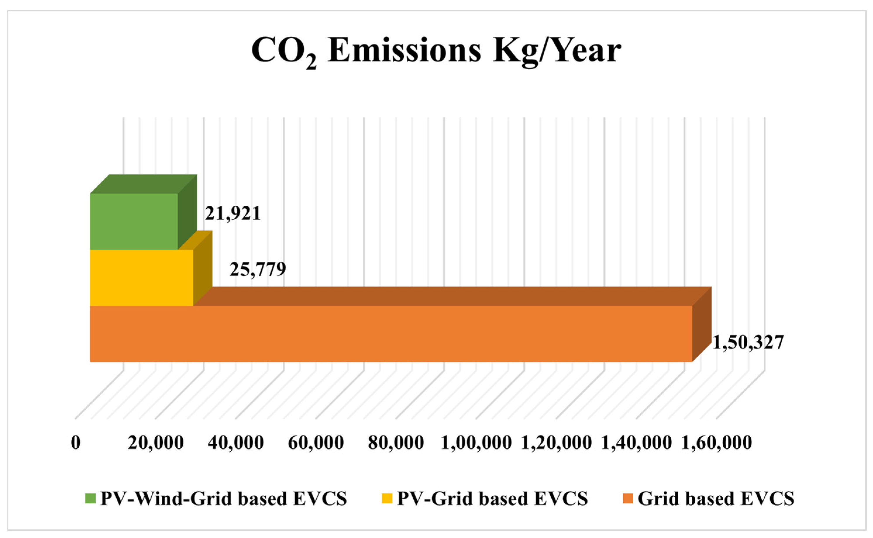
3.2. Environmental Analysis
4. Smart Monitoring of Distribution Networks Using µPMUs with EVCSs and DGs
- Type 1 only inject active power into the system;
- Type 2 only inject reactive power;
- Type 3 inject both active and reactive power;
- Type 4 inject active power but absorb reactive power.
- Scenario 1: IEEE 33-bus system without EVCSs and without integrating DGs (Base Case);
- Scenario 2: IEEE 33-bus system with EVCS load and without integrating DGs;
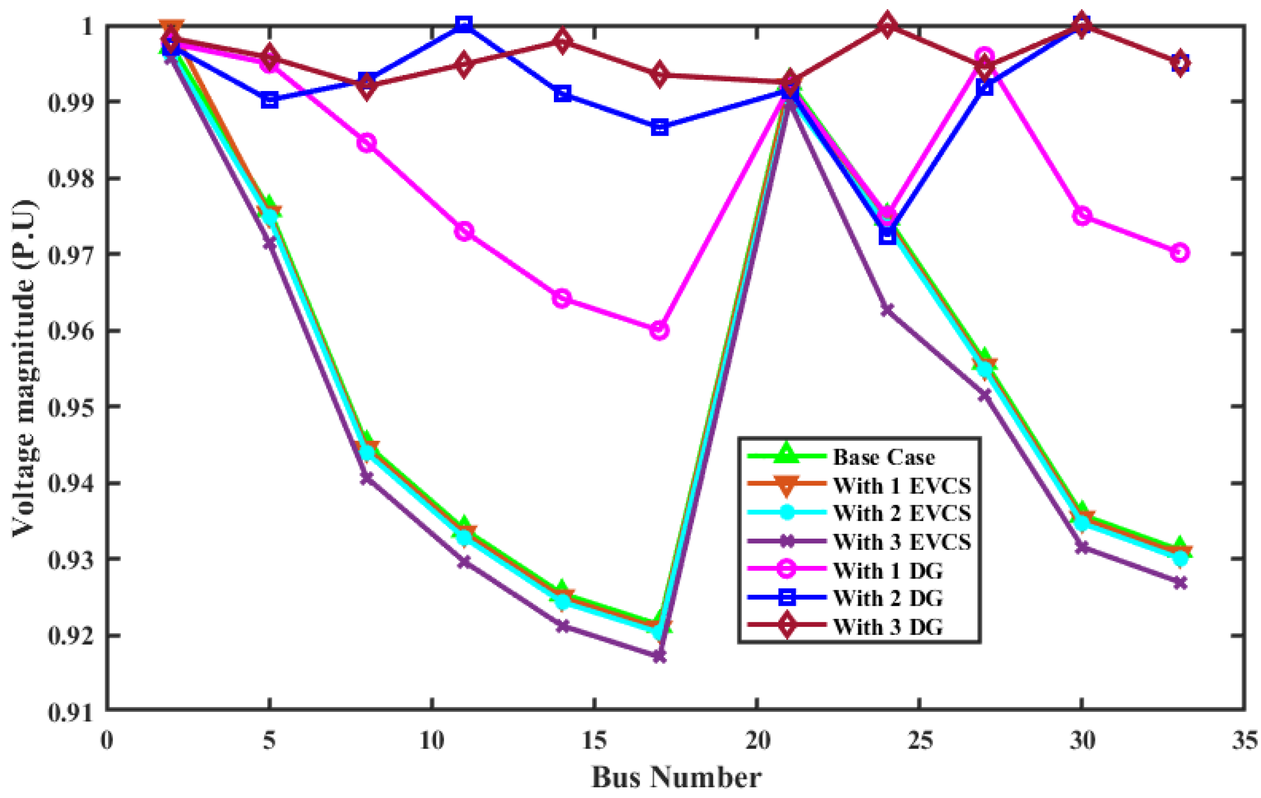
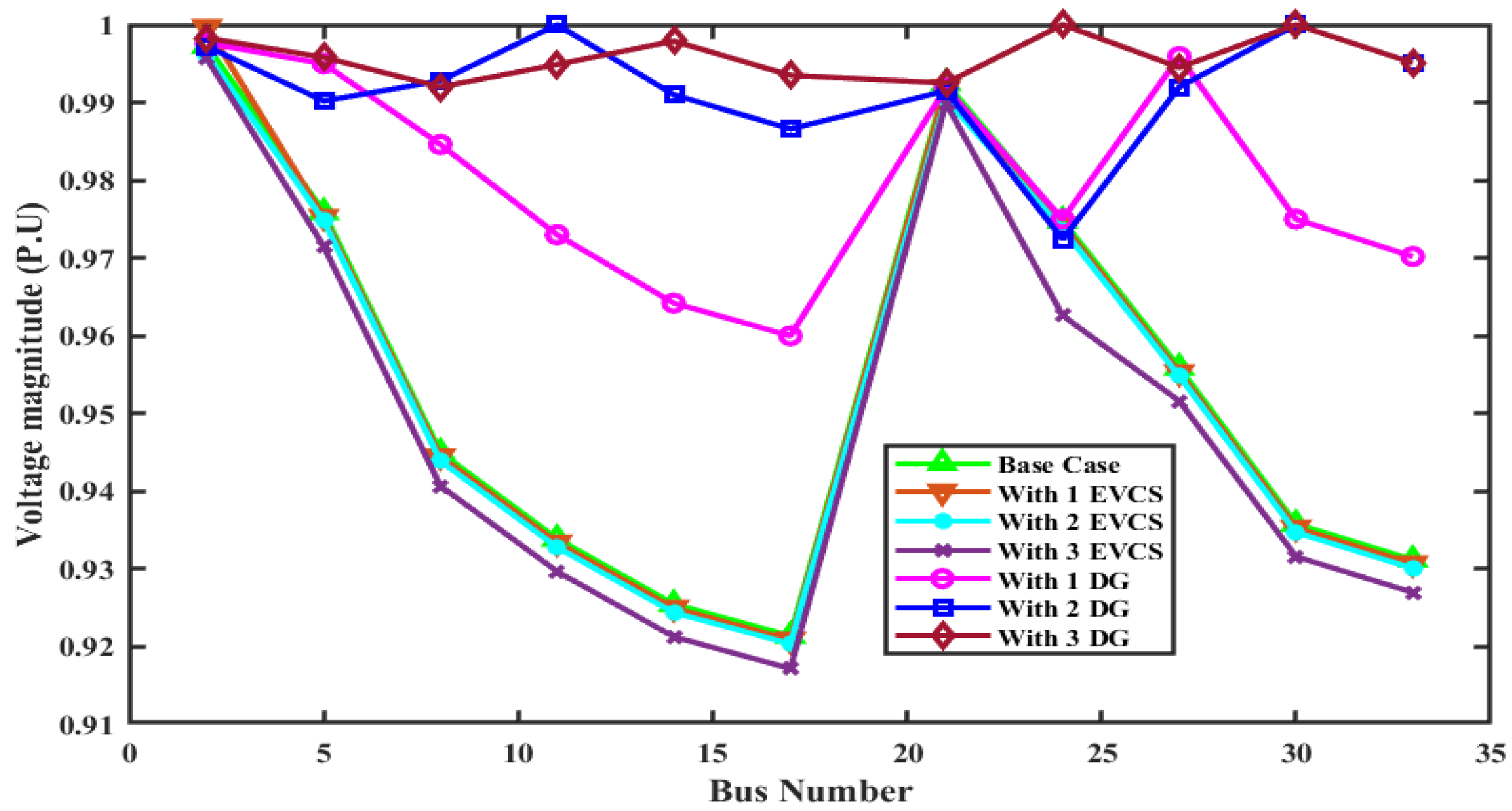
- Scenario 3: IEEE 33-bus system with EVCS load and type-1 DGs;
- Scenario 4: IEEE 33-bus system with EVCS load and type-2 DGs;
- Scenario 5: IEEE 33-bus system with EVCS load and type-3 DGs;
- Scenario 6: IEEE 33-bus system with EVCS load and type-4 DGs.
- Scenario 1: IEEE 33-bus system without EVCSs and without integrating DGs (Base Case).
- Scenario 2: IEEE 33-bus system with EVCS load and without integrating DGs
- Scenario 3: IEEE 33-bus system with EVCS load and type-1 DGs
| Type 1 | Voltage Magnitude (p.u) by Injecting Only Active Power | ||||||
|---|---|---|---|---|---|---|---|
| Bus No. | Base Case | 1 EVCS 975 kW at Bus 2 | 2 EVCSs 975 kW at Buses 2 and 19 | 3 EVCSs 975 kW at Buses 2, 19, and 25 | 1 DG with 2589.6 kW at Bus 6 | 2 DGs with 1898.7 kW at Bus 6 and 649.9 kW at Bus 14 | 3 DGs with 790 kW at Bus 13, 1070 kW at Bus 24, and 1010 kW at Bus 30 |
| 2 | 1 | 0.9994 | 0.9989 | 0.9983 | 0.9998 | 0.9998 | 1 |
| 5 | 0.9760 | 0.9754 | 0.9748 | 0.9709 | 0.9880 | 0.988 | 0.9874 |
| 8 | 0.9405 | 0.9399 | 0.9392 | 0.9351 | 0.9670 | 0.9751 | 0.9724 |
| 11 | 0.9274 | 0.9268 | 0.9262 | 0.9221 | 0.9543 | 0.9723 | 0.9716 |
| 14 | 0.9175 | 0.9169 | 0.9163 | 0.9121 | 0.9447 | 0.9729 | 0.9716 |
| 17 | 0.9127 | 0.9121 | 0.9114 | 0.9072 | 0.94 | 0.9683 | 0.9670 |
| 21 | 0.9952 | 0.9946 | 0.9930 | 0.9924 | 0.9940 | 0.9940 | 0.9942 |
| 24 | 0.9756 | 0.9750 | 0.9745 | 0.9616 | 0.9719 | 0.9718 | 0.9827 |
| 27 | 0.9531 | 0.9525 | 0.9519 | 0.9478 | 0.9793 | 0.9792 | 0.9780 |
| 30 | 0.9300 | 0.9294 | 0.9287 | 0.9246 | 0.9568 | 0.9567 | 0.9711 |
| 33 | 0.9246 | 0.9240 | 0.9234 | 0.9192 | 0.9516 | 0.9515 | 0.9660 |
| Type 1 | Voltage Magnitude (p.u) by Injecting Only Active Power | ||||||
|---|---|---|---|---|---|---|---|
| Bus No. | Base Case | 1 EVCS 975 kW at Bus 2 | 2 EVCSs 975 kW at Bus 2 and 19 | 3 EVCSs 975 kW at Buses 2, 19, and 25 | 1 DG with 2589.6 kW at Bus 6 | 2 DGs with 1898.7 kW at Bus 6 and 649.9 kW at Bus 14 | 3 DGs with 790 kW at Bus 13, 1070 kW at Bus 24, and 1010 kW at Bus 30 |
| 2 | 0.9973 | 0.9997 | 0.9962 | 0.9956 | 0.9976 | 0.99976 | 0.9983 |
| 5 | 0.9759 | 0.9753 | 0.9748 | 0.9715 | 0.995 | 0.995 | 0.9959 |
| 8 | 0.945 | 0.9445 | 0.9439 | 0.9407 | 0.9846 | 0.9954 | 0.992 |
| 11 | 0.9339 | 0.9334 | 0.9328 | 0.9297 | 0.973 | 0.9956 | 0.9949 |
| 14 | 0.9255 | 0.925 | 0.9244 | 0.9213 | 0.9642 | 1 | 0.0997 |
| 17 | 0.9214 | 0.9209 | 0.9204 | 0.9172 | 0.96 | 0.9956 | 0.9935 |
| 21 | 0.9925 | 0.992 | 0.9904 | 0.9899 | 0.9919 | 0.9919 | 0.9925 |
| 24 | 0.9748 | 0.9743 | 0.9737 | 0.9626 | 0.975 | 0.975 | 1 |
| 27 | 0.9559 | 0.9553 | 0.9548 | 0.9516 | 0.9959 | 0.9959 | 0.9945 |
| 30 | 0.9358 | 0.9353 | 0.9347 | 0.9316 | 0.975 | 0.975 | 1 |
| 33 | 0.9312 | 0.9307 | 0.9301 | 0.927 | 0.9702 | 0.9702 | 0.9951 |
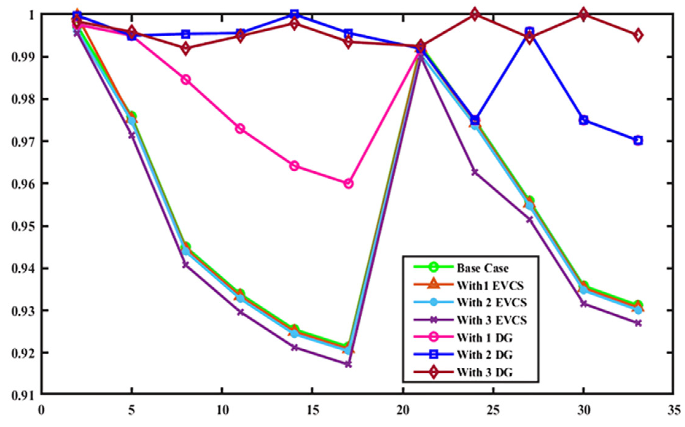
- Type 1: Injecting only active power.
- Scenario 4: IEEE 33-bus system with EVCS load and type-2 DGs
| Type 2 | Voltage Magnitude (p.u) by Injecting Only Active Power | ||||||
|---|---|---|---|---|---|---|---|
| Bus No. | Base Case | 1 EVCS 975 kW at Bus 2 | 2 EVCSs 975 kW at Bus 2 and 19 | 3 EVCSs 975 kW at Buses 2, 19, and 25 | 1 DG with 2589.6 kW at Bus 6 | 2 DGs with 1898.7 kW at Bus 6 and 649.9 kW at Bus 14 | 3 DGs with 790 kW at Bus 13, 1070 kW at Bus 24, and 1010 kW at Bus 30 |
| 2 | 1 | 0.9994 | 0.9989 | 0.9983 | 0.9987 | 0.9987 | 0.9989 |
| 5 | 0.9760 | 0.9754 | 0.9748 | 0.9709 | 0.9766 | 0.9777 | 0.9783 |
| 8 | 0.9405 | 0.9399 | 0.9392 | 0.9351 | 0.9471 | 0.9547 | 0.9541 |
| 11 | 0.9274 | 0.9268 | 0.9262 | 0.9221 | 0.9342 | 0.9463 | 0.9450 |
| 14 | 0.9175 | 0.9169 | 0.9163 | 0.9121 | 0.9243 | 0.9370 | 0.9383 |
| 17 | 0.9127 | 0.9121 | 0.9114 | 0.9072 | 0.9195 | 0.9322 | 0.9336 |
| 21 | 0.9952 | 0.9946 | 0.9930 | 0.9924 | 0.9928 | 0.9929 | 0.9930 |
| 24 | 0.9756 | 0.9750 | 0.9745 | 0.9616 | 0.9643 | 0.9648 | 0.9690 |
| 27 | 0.9531 | 0.9525 | 0.9519 | 0.9478 | 0.9617 | 0.9637 | 0.9638 |
| 30 | 0.9300 | 0.9294 | 0.9287 | 0.9246 | 0.9543 | 0.9540 | 0.9539 |
| 33 | 0.9246 | 0.9240 | 0.9234 | 0.9192 | 0.9491 | 0.9488 | 0.9487 |
| Type 2 | Voltage Magnitude (p.u) by Injecting Only Reactive Power | ||||||
|---|---|---|---|---|---|---|---|
| Bus No. | Base Case | 1 EVCS 975 kW at Bus 2 | 2 EVCSs 975 kW at Bus 2 and 19 | 3 EVCSs 975 kW at Buses 2, 19, and 25 | 1 DG with 2589.6 kW at Bus 6 | 2 DGs with 1898.7 kW at Bus 6 and 649.9 kW at Bus 14 | 3 DGs with 790 kW at Bus 13, 1070 kW at Bus 24, and 1010 kW at Bus 30 |
| 2 | 0.9973 | 0.9997 | 0.9962 | 0.9956 | 0.9968 | 0.99972 | 0.9983 |
| 5 | 0.9759 | 0.9753 | 0.9748 | 0.9715 | 0.9853 | 0.9901 | 0.9958 |
| 8 | 0.945 | 0.9445 | 0.9439 | 0.9407 | 0.9667 | 0.9921 | 0.992 |
| 11 | 0.9339 | 0.9334 | 0.9328 | 0.9297 | 0.9553 | 0.9987 | 0.9949 |
| 14 | 0.9255 | 0.925 | 0.9244 | 0.9213 | 0.9467 | 0.9923 | 0.9979 |
| 17 | 0.9214 | 0.9209 | 0.9204 | 0.9172 | 0.9425 | 0.988 | 0.9935 |
| 21 | 0.9925 | 0.992 | 0.9904 | 0.9899 | 0.991 | 0.9914 | 0.9925 |
| 24 | 0.9748 | 0.9743 | 0.9737 | 0.9626 | 0.9698 | 0.9724 | 1 |
| 27 | 0.9559 | 0.9553 | 0.9548 | 0.9516 | 0.9842 | 0.9917 | 0.9945 |
| 30 | 0.9358 | 0.9353 | 0.9347 | 0.9316 | 1 | 1 | 1 |
| 33 | 0.9312 | 0.9307 | 0.9301 | 0.927 | 0.9951 | 0.9951 | 0.9951 |
- Type 1: Injecting only reactive power.
- Scenario 5: IEEE 33-bus system with EVCS load and type-3 DGs
| Type 3 | Voltage Magnitude (p.u) by Injecting Only Active and Reactive Power | ||||||
|---|---|---|---|---|---|---|---|
| Bus No. | Base Case | 1 EVCS 975 kW at Bus 2 | 2 EVCSs 975 kW at Bus 2 and 19 | 3 EVCSs 975 kW at Buses 2, 19, and 25 | 1 DG with 2589.6 kW at Bus 6 | 2 DGs with 1898.7 kW at Bus 6 and 649.9 kW at Bus 14 | 3 DGs with 790 kW at Bus 13, 1070 kW at Bus 24, and 1010 kW at Bus 30 |
| 2 | 1 | 0.9994 | 0.9989 | 0.9983 | 1.0004 | 1.0002 | 1.0006 |
| 5 | 0.9760 | 0.9754 | 0.9748 | 0.9709 | 0.9956 | 0.9945 | 0.9936 |
| 8 | 0.9405 | 0.9399 | 0.9392 | 0.9351 | 0.9826 | 0.9971 | 0.9878 |
| 11 | 0.9274 | 0.9268 | 0.9262 | 0.9221 | 0.9702 | 1.0035 | 0.9892 |
| 14 | 0.9175 | 0.9169 | 0.9163 | 0.9121 | 0.9607 | 0.9944 | 0.9911 |
| 17 | 0.9127 | 0.9121 | 0.9114 | 0.9072 | 0.9561 | 0.9899 | 0.9866 |
| 21 | 0.9952 | 0.9946 | 0.9930 | 0.9924 | 0.9945 | 0.9944 | 0.9947 |
| 24 | 0.9756 | 0.9750 | 0.9745 | 0.9616 | 0.9753 | 0.9745 | 0.9913 |
| 27 | 0.9531 | 0.9525 | 0.9519 | 0.9478 | 0.9947 | 0.9987 | 0.9905 |
| 30 | 0.9300 | 0.9294 | 0.9287 | 0.9246 | 0.9726 | 1.0131 | 0.9933 |
| 33 | 0.9246 | 0.9240 | 0.9234 | 0.9192 | 0.9675 | 0.0082 | 0.9883 |
| Type 3 | Voltage Magnitude (p.u) by Injecting Only Active and Reactive Power | ||||||
|---|---|---|---|---|---|---|---|
| Bus No. | Base Case | 1 EVCS 975 kW at Bus 2 | 2 EVCSs 975 kW at Bus 2 and 19 | 3 EVCSs 975 kW at Buses 2, 19, and 25 | 1 DG with 2589.6 kW at Bus 6 | 2 DGs with 1898.7 kW at Bus 6 and 649.9 kW at Bus 14 | 3 DGs with 790 kW at Bus 13, 1070 kW at Bus 24, and 1010 kW at Bus 30 |
| 2 | 0.9973 | 0.9997 | 0.9962 | 0.9956 | 0.9976 | 0.9972 | 0.9983 |
| 5 | 0.9759 | 0.9753 | 0.9748 | 0.9715 | 0.995 | 0.9902 | 0.9958 |
| 8 | 0.945 | 0.9445 | 0.9439 | 0.9407 | 0.9846 | 0.9928 | 0.992 |
| 11 | 0.9339 | 0.9334 | 0.9328 | 0.9297 | 0.973 | 1 | 0.9949 |
| 14 | 0.9255 | 0.925 | 0.9244 | 0.9213 | 0.9642 | 0.991 | 0.9979 |
| 17 | 0.9214 | 0.9209 | 0.9204 | 0.9172 | 0.96 | 0.9866 | 0.9935 |
| 21 | 0.9925 | 0.992 | 0.9904 | 0.9899 | 0.9919 | 0.9915 | 0.9925 |
| 24 | 0.9748 | 0.9743 | 0.9737 | 0.9626 | 0.975 | 0.9724 | 1 |
| 27 | 0.9559 | 0.9553 | 0.9548 | 0.9516 | 0.9959 | 0.992 | 0.9945 |
| 30 | 0.9358 | 0.9353 | 0.9347 | 0.9316 | 0.975 | 1 | 1 |
| 33 | 0.9312 | 0.9307 | 0.9301 | 0.927 | 0.9702 | 0.9951 | 0.9951 |
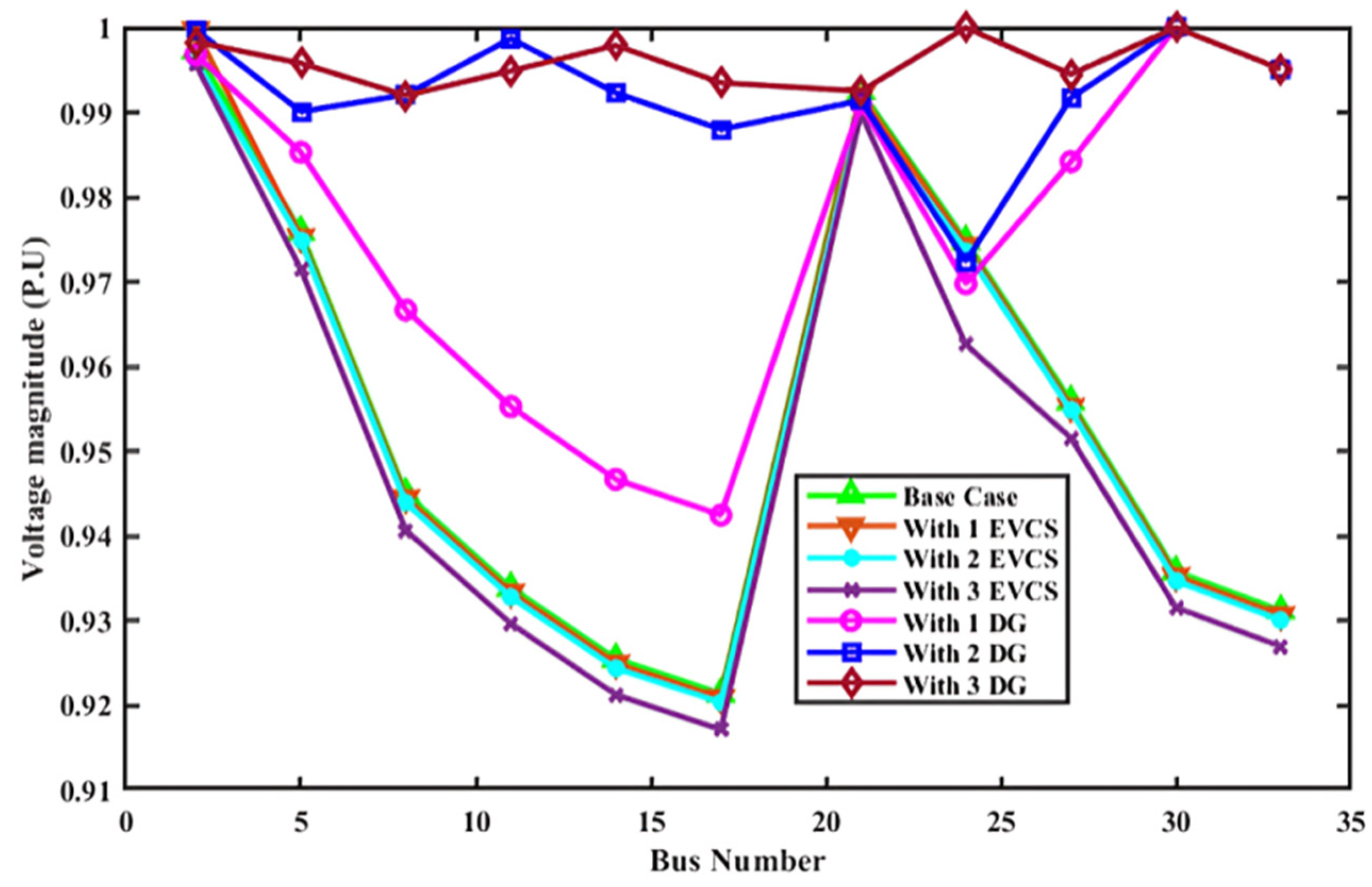
- Type 3: Injecting active and reactive power.
- Scenario 6: IEEE 33-bus system with EVCS load and type-4 DGs
- Type 4: Injecting only reactive power.
| Execution Time Using Forward/Backward Algorithm (seconds) | Execution Time Using µPMUs (seconds) | |
|---|---|---|
| Base Case | 19.59 | 5.93 |
| 1 EVCS | 19.64 | 5.64 |
| 2 EVCS | 19.75 | 5.65 |
| 3 EVCS | 19.98 | 5.78 |
| Type 1 | ||
| 1 DG | 19.76 | 5.68 |
| 2 DGs | 19.95 | 5.80 |
| 3 DGs | 19.98 | 6.25 |
| Type 2 | ||
| 1 DG | 19.79 | 5.68 |
| 2 DGs | 19.88 | 5.80 |
| 3 DGs | 19.89 | 6.00 |
| Type 3 | ||
| 1 DG | 19.82 | 5.89 |
| 2 DGs | 19.88 | 5.80 |
| 3 DGs | 19.92 | 6.06 |
| Type 4 | ||
| 1 DG | 19.07 | 5.95 |
| 2 DGs | 20.07 | 6.03 |
| 3 DGs | 21.22 | 6.12 |
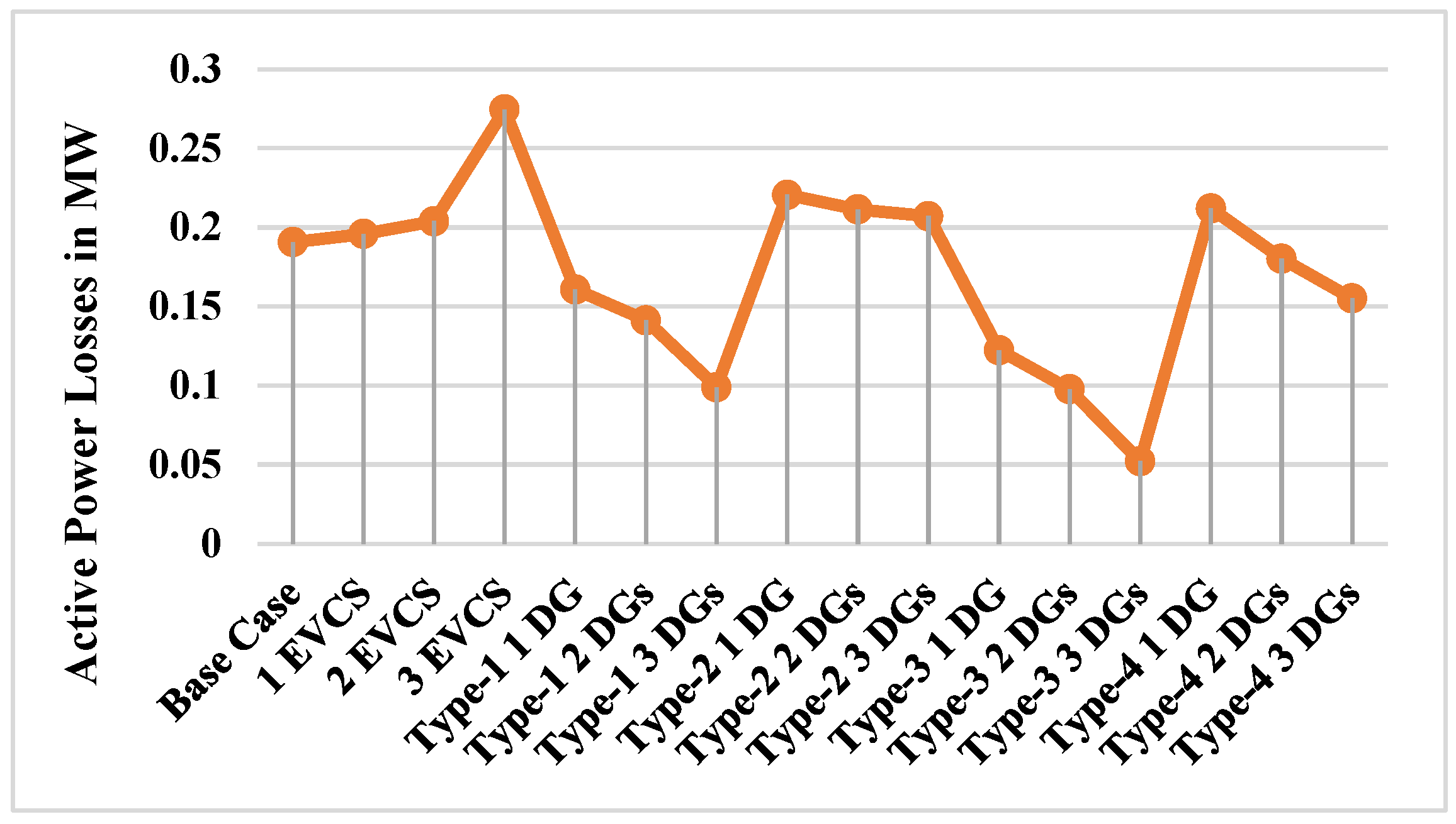
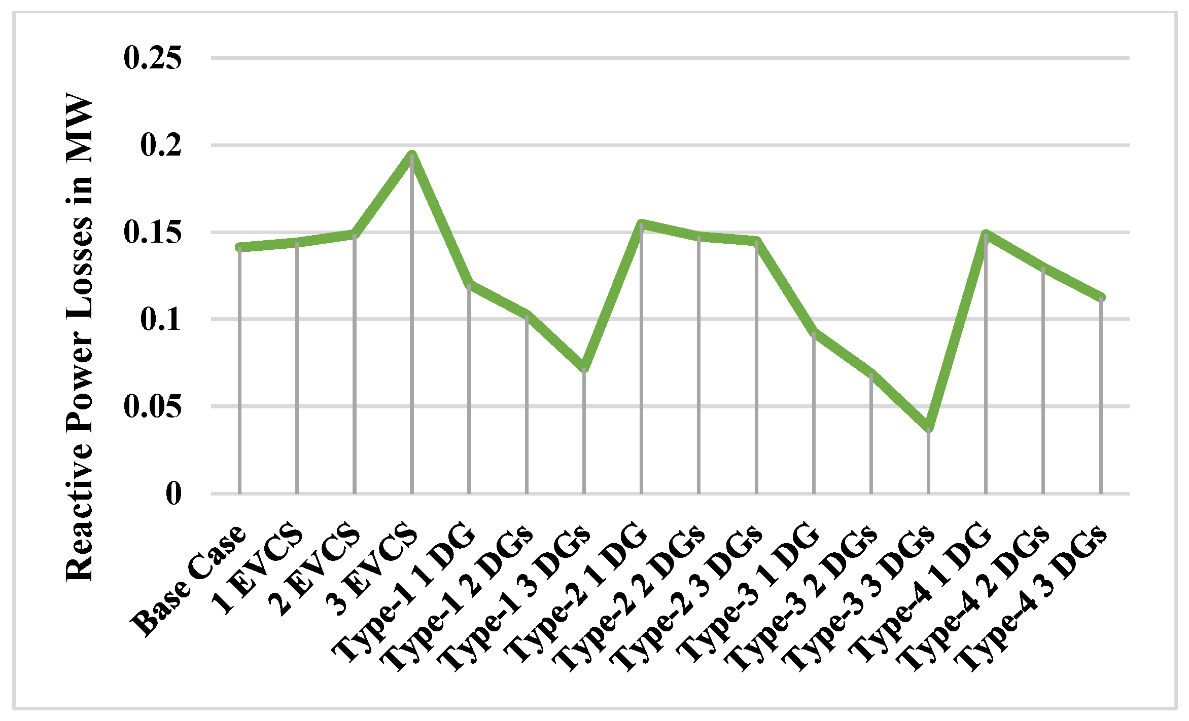
| Installed Capacity of DG | Total Active Power Loss (MW) | Total Reactive Power Loss (MW) | Loss Reduction in % | |
|---|---|---|---|---|
| Base Case | ---- | 0.19061 | 0.14123 | ---- |
| 1 EVCS | 975 kW at bus 2 | 0.19578 | 0.14393 | |
| 2 EVCSs | 975 kW at bus 2 and bus 19 | 0.20382 | 0.14884 | |
| 3 EVCSs | 975 kW at bus 2, bus 19, and bus 25 | 0.27459 | 0.19431 | |
| Type 1 | ||||
| 1 DG | 2589.6 kW at bus 6 | 0.16078 | 0.11992 | 41.44% |
| 2 DGs | 1898.7 kW at bus 6 649.9 kW at bus 14 | 0.14121 | 0.10256 | 48.57% |
| 3 DGs | 790 kW at bus 13 1070 kW at bus 24 1010 kW at bus 30 | 0.09893 | 0.07198 | 63.97% |
| Type 2 | ||||
| 1 DG | 1230 kvar at bus 30 | 0.22053 | 0.15477 | 19.68% |
| 2 DGs | 430 kvar at bus 12 1040 kvar at bus 30 | 0.21135 | 0.14741 | 23.03% |
| 3 DGs | 360 kvar at bus 13 510 kvar at bus 24 1020 kvar at bus 30 | 0.20708 | 0.14479 | 24.58% |
| Type 3 | ||||
| 1 DG | 2558.2 kW/1761.1 kvar at bus 6 | 0.12233 | 0.092437 | 55.44% |
| 2 DGs | 1171.2 kW/188.1 kvar at bus 11 1095.4 kW/1667.0 kvar at bus 30 | 0.09763 | 0.06890 | 64.44% |
| 3 DGs | 537.8 kW/597.3 kvar at bus 13 1058.9 kW/832.9 kvar at bus 24 967.7 kW/832.6 kvar at bus 30 | 0.05219 | 0.03769 | 80.99% |
| Type 4 | ||||
| 1 DG | 1095 kW/−235 kvar at bus 13 | 0.211983 | 0.14876 | 22.8% |
| 2 DGs | 1171.2 kW/−188.1 kvar at bus 11 1095.4 kW/−266.0 kvar at bus 30 | 0.180175 | 0.12967 | 34.38% |
| 3 DGs | 663.07 kW/−217.9 kvar at bus 13 1400 kW/−460.16 kvar at bus 24 717.08 kW/ −235.69 kvar at bus 30 | 0.15506 | 0.11258 | 43.53% |
5. Conclusions
Author Contributions
Funding
Data Availability Statement
Conflicts of Interest
Abbreviations
| RE | Renewable Energy |
| µPMU | Micro Phasor Measurement Unit |
| EVCS | Electric Vehicle Charging Station |
| CAGR | Compound Annual Growth Rate |
| BU | Billion Units |
| MU | Million Units |
| DG | Distributed Generator |
| PV | Photovoltaic |
| V2G | Vehicle to Grid |
| COE | Cost of Energy |
| NPV | Net Present Value |
References
- Electric Power Survey Report 2022. Available online: https://cea.nic.in/wpcontent/uploads/ps___lf/2022/11/20th_EPS____Report___Final___16.11.2022.pdf (accessed on 16 November 2022).
- Final Report on National Electricity Plan 2022–2032. Available online: https://mnre.gov.in/policies-and-regulations/policies-and-guidelines/centre (accessed on 12 March 2024).
- Report on All India Installed Capacity. Available online: https://cea.nic.in/wp-content/uploads/installed/2023/05/IC_May_2023.pdf (accessed on 31 May 2023).
- Mandal, S.; Das, B.K.; Hoque, N. Optimum sizing of a stand-alone hybrid energy system for rural electrification in Bangladesh. J. Clean. Prod. 2018, 200, 12–27. [Google Scholar] [CrossRef]
- Akram, F.; Asghar, F.; Majeed, M.A.; Amjad, W.; Manzoor, M.O.; Munir, A. Techno-economic optimization analysis of stand-alone renewable energy system for remote areas. Sustain. Energy Technol. Assess. 2020, 38, 100673. [Google Scholar] [CrossRef]
- Kiwan, S.; Al-Nimr, M.; Salim, I. A hybrid solar chimney/photovoltaic thermal system for direct electric power production and water distillation. Sustain. Energy Technol. Assess. 2020, 38, 100680. [Google Scholar] [CrossRef]
- Carvajal-Romo, G.; Valderrama-Mendoza, M.; Rodríguez-Urrego, D.; Rodríguez-Urrego, L. Assessment of solar and wind energy potential in La Guajira, Colombia: Current status, and future prospects. Sustain. Energy Technol. Assess. 2019, 36, 100531. [Google Scholar] [CrossRef]
- Nandi, S.K.; Ghosh, H.R. A wind–PV-battery hybrid power system at Sitakunda in Bangladesh. Energy Policy 2009, 37, 3659–3664. [Google Scholar] [CrossRef]
- Darus, Z.; Hashim, N.A.; Manan, S.A.; Rahman, M.A.; Maulud, K.A.; Karim, O.A. The development of hybrid integrated renewable energy system (wind and solar) for sustainable living at Perhentian Island, Malaysia. Eur. J. Soc. Sci. 2009, 9, 557–563. [Google Scholar]
- Das, H.S.; Tan, C.W.; Yatim, A.; Lau, K.Y. Feasibility analysis of hybrid photovoltaic/battery/fuel cell energy system for an indigenous residence in East Malaysia. Renew. Sustain. Energy Rev. 2017, 76, 1332–1347. [Google Scholar] [CrossRef]
- Isa, N.M.; Das, H.S.; Tan, C.W.; Yatim, A.; Lau, K.Y. A techno-economic assessment of a combined heat and power photovoltaic/fuel cell/battery energy system in Malaysia hospital. Energy 2016, 112, 75–90. [Google Scholar] [CrossRef]
- Eid, A. Utility integration of PV-wind-fuel cell hybrid distributed generation systems under variable load demands. Int. J. Electr. Power Energy Syst. 2014, 62, 689–699. [Google Scholar] [CrossRef]
- Heydari, A.; Askarzadeh, A. Techno-economic analysis of a PV/biomass/fuel cell energy system considering different fuel cell system initial capital costs. Sol. Energy 2016, 133, 409–420. [Google Scholar] [CrossRef]
- Bukar, A.L.; Tan, C.W. A review on stand-alone photovoltaic-wind energy system with fuel cell: System optimization and energy management strategy. J. Clean. Prod. 2019, 221, 73–88. [Google Scholar] [CrossRef]
- Tan, Q.; Mei, S.; Ye, Q.; Ding, Y.; Zhang, Y. Optimization model of a combined wind–PV–thermal dispatching system under carbon emissions trading in China. J. Clean. Prod. 2019, 225, 391–404. [Google Scholar] [CrossRef]
- Murugaperumal, K.; Srinivasn, S.; Prasad, G.S. Optimum design of hybrid renewable energy system through load forecasting and different operating strategies for rural electrification. Sustain. Energy Technol. Assess. 2019, 37, 100613. [Google Scholar] [CrossRef]
- Raghuwanshi, S.S.; Arya, R. Reliability evaluation of stand-alone hybrid photovoltaic energy system for rural healthcare centre. Sustain. Energy Technol. Assess. 2020, 37, 100624. [Google Scholar] [CrossRef]
- Mhandu, S.R.; Longe, O.M. Techno-Economic Analysis of Hybrid PV-Wind-Diesel-Battery Standalone and Grid-Connected Microgrid for Rural Electrification in Zimbabwe. In Proceedings of the 2022 IEEE Nigeria 4th International Conference on Disruptive Technologies for Sustainable Development (NIGERCON), Lagos, Nigeria, 5–7 April 2022. [Google Scholar]
- Nienhueser, I.A.; Qiu, Y. Economic and environmental impacts of providing renewable energy for electric vehicle charging—A choice experiment study. Appl. Energy 2016, 180, 256–268. [Google Scholar] [CrossRef]
- Shaaban, M.F.; El-Saadany, E.F. Accommodating high penetrations of PEVs and renewable DG considering uncertainties in distribution systems. IEEE Trans. Power Syst. 2013, 29, 259–270. [Google Scholar] [CrossRef]
- Rahman, M.M.; Al-Ammar, E.A.; Das, H.S.; Ko, W. Technical Assessment of Plug-In Hybrid Electric Vehicle Charging Scheduling for Peak Reduction. In Proceedings of the 2019 10th International Renewable Energy Congress (IREC), Sousse, Tunisia, 26–28 March 2019. [Google Scholar]
- Shafiq, S.; Al-Awami, A.T. Reliability and economic assessment of renewable micro-grid with V2G electric vehicles coordination. In Proceedings of the 2015 IEEE Jordan Conference on Applied Electrical Engineering and Computing Technologies (AEECT), Amman, Jordan, 3–5 November 2015. [Google Scholar]
- Habib, S.; Kamran, M.; Rashid, U. Impact analysis of vehicleto- grid technology and charging strategies of electric vehicles on distribution networks—A review. J. Power Sources 2015, 277, 205–214. [Google Scholar] [CrossRef]
- Fathabadi, H. Novel solar powered electric vehicle charging station with the capability of vehicle-to-grid. Sol. Energy 2017, 142, 136–143. [Google Scholar] [CrossRef]
- Hafez, O.; Bhattacharya, K. Optimal design of electric vehicle charging stations considering various energy resources. Renew. Energy 2017, 107, 576–589. [Google Scholar] [CrossRef]
- Nazari, M.A.; Blazek, V.; Prokop, L.; Misak, S.; Prabaharan, N. Electric vehicle charging by use of renewable energy technologies: A comprehensive and updated review. Comput. Electr. Eng. 2024, 118, 109401. [Google Scholar] [CrossRef]
- Marinescu, C. Progress in the development and implementation of residential EV charging stations based on renewable energy sources. Energies 2022, 16, 179. [Google Scholar] [CrossRef]
- Ihm, J.; Amghar, B.; Chun, S.; Park, H. Optimum design of an electric vehicle charging station using a renewable power generation system in South Korea. Sustainability 2023, 15, 9931. [Google Scholar] [CrossRef]
- Narasipuram, R.P.; Mopidevi, S. A technological overview & design considerations for developing electric vehicle charging stations. J. Energy Storage 2021, 43, 103225. [Google Scholar] [CrossRef]
- Ashraf, I.; Al Sharari, H.; Tariq, M.; Tabish, S. Grid-Assisted Rooftop Solar PV System: A Step toward Green Medina, KSA. Smart Sci. 2018, 7, 130–138. [Google Scholar] [CrossRef]
- Moria, H. Techno-Economic Optimization of Solar/Wind Turbine System for Remote Mosque in Saudi Arabia Highway: Case Study. Int. J. Eng. Res. 2019, 8, 78–84. [Google Scholar] [CrossRef]
- Alghamdi, A.H.S. Technical and Economic Analysis of Solar Energy Application for a Hospital Building in Dammam, Saudi Arabia. Master’s Thesis, Auckland University of Technology, Auckland, New Zealand, 2018. [Google Scholar]
- HOMER Grid. 2020. Available online: https://www.homerenergy.com/products/pro/docs/latest/index.html (accessed on 10 October 2020).
- Koski, J. Defectiveness of weighting method in multicriterion optimization of structures. Commun. Appl. Numer. Methods 1985, 1, 333–337. [Google Scholar] [CrossRef]
- Shah, D.N. Synchrophasor Technology: Addressing Integration of Renewable with Synchronous Grid by Real Time Monitoring through WAMS. In Proceedings of the 2nd International Conference on Large-Scale Grid Integration of Renewable Energyin India, New Delhi, India, 4–6 September 2019; Available online: https://regridintegrationindia.org/wp-content/uploads/sites/14/2019/11/10A_2_RE_India19_029_paper_Shah_D.pdf (accessed on 17 September 2024).
- Khalil, L.; Bhatti, K.L.; Awan, M.A.I.; Riaz, M.; Khalil, K.; Alwaz, N. Optimization and designing of hybrid power system using HOMER pro. Mater. Today Proc. 2020, 47, S110–S115. [Google Scholar] [CrossRef]
- Himabindu, N.; Hampannavar, S.; Deepa, B.; Longe, O.M.; Mansani, S.; Komanapalli, V. Assessment of microgrid integrated biogas–photovoltaic powered Electric Vehicle Charging Station (EVCS) for sustainable future. Energy Rep. 2023, 9, 139–143. [Google Scholar] [CrossRef]
- Final Report on the Study and Development of Emission Factor (Ef) for Indian Electrical Grid in 2021–2022. Available online: https://cea.nic.in/wpcontent/uploads/baseline/2023/01/Approved_report_emission__2021_22.pdf (accessed on 16 March 2024).
- Himabindu, N.; Hamoannavar, S.; Deppa, B.; Swapna, M. Analysis of microgrid integrated Photovoltaic (PV) Powered Electric Vehicle Charging Stations (EVCS) under different solar irradiation conditions in India: A way towards sustainable development and growth. Energy Rep. 2021, 7, 8534–8547. [Google Scholar] [CrossRef]
- Central Electricity Authority (India), Draft National Electricity Plan (Volume 1: Generation). 2022. Available online: http://www.cea.nic.in/reports/committee/nep/nep_dec.pdf (accessed on 8 September 2022).
- State Wise Estimated Solar Power Potential in the Country; Tech. Rep. No. 22/02/2014-15/Solar-RD (Misc.); Solar R&D Division, Ministry of New & Renewable Energy, Government of India: New Delhi, India, 2014; Available online: http://www.indiaenvironmentportal.org.in/files/file/Statewise-Solar-Potential-NISE_0.pdf (accessed on 9 March 2024).
- NIWE. Estimation of Installable Wind Power Potential at 80 m Level in India; Technical Report; National Institute of Wind Energy, India: Tamil Nadu, India, 2024; Available online: https://niwe.res.in/assets/Docu/India's_Wind_Potential_Atlas_at_120m_agl.pdf (accessed on 9 March 2024).
- Pradeep, S. Role of monetary policy on CO2 emissions in India. SN Bus. Econ. 2021, 2, 3. [Google Scholar] [CrossRef]
- Hampannavar, S.; Deepa, B.; Swapna, M. Micro Phasor Measurement Unit (μPMU) Placement for Maximum Observability in Smart Distribution Network. In Proceedings of the 2021 IEEE PES/IAS PowerAfrica, Virtual, 23–27 August 2021. [Google Scholar]
| Parameters | Stand-Alone System | Grid-Connected System | |||
|---|---|---|---|---|---|
| PV Analysis Values | PV–Wind Analysis Values | PV–Grid Analysis Values | PV–Wind–Grid Analysis Values | ||
| Technological Parameter | kWh generation | 502,516 kWh | 498,417 kWh | 502,516 kWh | 497,281 kWh |
| Economic Parameter | COE ($) | 1.44 | 1.13 | 0.517 | 0.385 |
| NPC ($) | 4.42 M | 3.47 M | 2.78 M | 2.45 M | |
| Initial Cost ($) | 2.65 M | 2.32 M | 1.88 M | 1.83 M | |
| Operating Cost ($) | 136,600 | 89,345 | 70,015 | 47,678 | |
| Environmental Parameter | CO2 Emissions (kg/year) | -- | -- | 25,779 | 21,921 |
| Scenarios | Bus Number and Size | Active Power Loss (Mw) | Reactive Power Loss (MVar) |
|---|---|---|---|
| Base case | --- | 0.19061 | 0.14123 |
| 1 EVCS | 975 kW at bus 2 | 0.19578 | 0.14393 |
| 2 EVCSs | 975 kW at bus 2 and bus 19 | 0.20382 | 0.14884 |
| 3 EVCSs | 975 kW at bus 2, bus 19, and bus 25 | 0.27459 | 0.19431 |
| Type 4 | Voltage Magnitude (p.u) by Injecting Only Active Power and Absorbing Reactive Power | ||||||
|---|---|---|---|---|---|---|---|
| Bus No. | Base Case | 1 EVCS 975 kW at Bus 2 | 2 EVCSs 975 kW at Buses 2 and 19 | 3 EVCSs 975 kW at Buses 2, 19, and 25 | 1 DG with 2589.6 kW at Bus 6 | 2 DGs with 1898.7 kW at Bus 6 and 649.9 kW at Bus 14 | 3 DGs with 790 kW at Bus 13, 1070 kW at Bus 24, and 1010 kW at Bus 30 |
| 2 | 1 | 0.9994 | 0.9989 | 0.9983 | 0.9989 | 0.9995 | 0.9997 |
| 5 | 0.9760 | 0.9754 | 0.9748 | 0.9709 | 0.9772 | 0.9839 | 0.9828 |
| 8 | 0.9405 | 0.9399 | 0.9392 | 0.9351 | 0.9576 | 0.9713 | 0.9588 |
| 11 | 0.9274 | 0.9268 | 0.9262 | 0.9221 | 0.9587 | 0.9741 | 0.9538 |
| 14 | 0.9175 | 0.9169 | 0.9163 | 0.9121 | 0.9604 | 0.9646 | 0.9504 |
| 17 | 0.9127 | 0.9121 | 0.9114 | 0.9072 | 0.9557 | 0.9600 | 0.9458 |
| 21 | 0.9952 | 0.9946 | 0.9930 | 0.9924 | 0.9930 | 0.9937 | 0.9938 |
| 24 | 0.9756 | 0.9750 | 0.9745 | 0.9616 | 0.9656 | 0.9697 | 0.9802 |
| 27 | 0.9531 | 0.9525 | 0.9519 | 0.9478 | 0.9593 | 0.9744 | 0.9674 |
| 30 | 0.9300 | 0.9294 | 0.9287 | 0.9246 | 0.9363 | 0.9655 | 0.9529 |
| 33 | 0.9246 | 0.9240 | 0.9234 | 0.9192 | 0.9310 | 0.9603 | 0.9477 |
| Type 4 | Voltage Magnitude (p.u) by Injecting Active Power and Absorbing Reactive Power | ||||||
|---|---|---|---|---|---|---|---|
| Bus No. | Base Case | 1 EVCS 975 kW at Bus 2 | 2 EVCSs 975 kW at Buses 2 and 19 | 3 EVCSs 975 kW at Buses 2, 19, and 25 | 1 DG with 2589.6 kW at Bus 6 | 2 DGs with 1898.7 kW at Bus 6 and 649.9 kW at Bus 14 | 3 DGs with 790 kW at Bus 13, 1070 kW at Bus 24, and 1010 kW at Bus 30 |
| 2 | 0.9973 | 0.9997 | 0.9962 | 0.9956 | 0.9964 | 0.9972 | 0.9983 |
| 5 | 0.9759 | 0.9753 | 0.9748 | 0.9715 | 0.9807 | 0.9902 | 0.9958 |
| 8 | 0.945 | 0.9445 | 0.9439 | 0.9407 | 0.9781 | 0.9928 | 0.992 |
| 11 | 0.9339 | 0.9334 | 0.9328 | 0.9297 | 0.9887 | 1 | 0.9949 |
| 14 | 0.9255 | 0.925 | 0.9244 | 0.9213 | 0.9979 | 0.991 | 0.9979 |
| 17 | 0.9214 | 0.9209 | 0.9204 | 0.9172 | 0.9935 | 0.9866 | 0.9935 |
| 21 | 0.9925 | 0.992 | 0.9904 | 0.9899 | 0.9907 | 0.9915 | 0.9925 |
| 24 | 0.9748 | 0.9743 | 0.9737 | 0.9626 | 0.9675 | 0.9724 | 1 |
| 27 | 0.9559 | 0.9553 | 0.9548 | 0.9516 | 0.9688 | 0.992 | 0.9945 |
| 30 | 0.9358 | 0.9353 | 0.9347 | 0.9316 | 0.9484 | 1 | 1 |
| 33 | 0.9312 | 0.9307 | 0.9301 | 0.927 | 0.9438 | 0.9951 | 0.9951 |
Disclaimer/Publisher’s Note: The statements, opinions and data contained in all publications are solely those of the individual author(s) and contributor(s) and not of MDPI and/or the editor(s). MDPI and/or the editor(s) disclaim responsibility for any injury to people or property resulting from any ideas, methods, instructions or products referred to in the content. |
© 2024 by the authors. Published by MDPI on behalf of the World Electric Vehicle Association. Licensee MDPI, Basel, Switzerland. This article is an open access article distributed under the terms and conditions of the Creative Commons Attribution (CC BY) license (https://creativecommons.org/licenses/by/4.0/).
Share and Cite
B, D.; Hampannavar, S.; Mansani, S. Smart Monitoring of Microgrid-Integrated Renewable-Energy-Powered Electric Vehicle Charging Stations Using Synchrophasor Technology. World Electr. Veh. J. 2024, 15, 432. https://doi.org/10.3390/wevj15100432
B D, Hampannavar S, Mansani S. Smart Monitoring of Microgrid-Integrated Renewable-Energy-Powered Electric Vehicle Charging Stations Using Synchrophasor Technology. World Electric Vehicle Journal. 2024; 15(10):432. https://doi.org/10.3390/wevj15100432
Chicago/Turabian StyleB, Deepa, Santoshkumar Hampannavar, and Swapna Mansani. 2024. "Smart Monitoring of Microgrid-Integrated Renewable-Energy-Powered Electric Vehicle Charging Stations Using Synchrophasor Technology" World Electric Vehicle Journal 15, no. 10: 432. https://doi.org/10.3390/wevj15100432
APA StyleB, D., Hampannavar, S., & Mansani, S. (2024). Smart Monitoring of Microgrid-Integrated Renewable-Energy-Powered Electric Vehicle Charging Stations Using Synchrophasor Technology. World Electric Vehicle Journal, 15(10), 432. https://doi.org/10.3390/wevj15100432