StegNet: Mega Image Steganography Capacity with Deep Convolutional Network

Abstract

Traditional image steganography often leans interests towards safely embedding hidden information into cover images with payload capacity almost neglected. This paper combines recent deep convolutional neural network methods with image-into-image steganography. It successfully hides the same size images with a decoding rate of 98.2% or bpp (bits per pixel) of 23.57 by changing only 0.76% of the cover image on average. Our method directly learns end-to-end mappings between the cover image and the embedded image and between the hidden image and the decoded image. We further show that our embedded image, while with mega payload capacity, is still robust to statistical analysis.

1. Introduction

Image steganography, aiming at delivering a modified cover image to secretly transfer hidden information inside with little awareness of the third-party supervision, is a classical computer vision and cryptography problem. Traditional image steganography algorithms go to their great length to hide information into the cover image while little consideration is tilted to payload capacity, also known as the ratio between hidden and total information transferred. The payload capacity is one significant factor to steganography methods because if more information is to be hidden in the cover, the visual appearance of the cover is altered further and thus the risk of detection is higher (The source code is available at: https://github.com/adamcavendish/StegNet-Mega-Image-Steganography-Capacity-with-Deep-Convolutional-Network).

The most commonly used image steganography for hiding large files during transmission is embedding a RAR archive (Roshal ARchive file format) after a JPEG (Joint Photographic Experts Group) file. In such way, it can store an infinite amount of extra information theoretically. However, the carrier file must be transmitted as it is, since any third-party alteration to the carrier is going to destroy all the hidden information in it, even just simply read out the image and save it again will corrupt the hidden information.

To maximize the payload capacity while still resistible to simple alterations, pixel level steganography is majorly used, in which LSB (least significant bits) method [1], BPCS [2] (Bit Plane Complexity Segmentation), and their extensions are in dominant. LSB-based methods can achieve a payload capacity of up to 50%, or otherwise, a vague outline of the hidden image would be exposed (see Figure 1). However, most of these methods are vulnerable to statistical analysis, and therefore it can be easily detected.

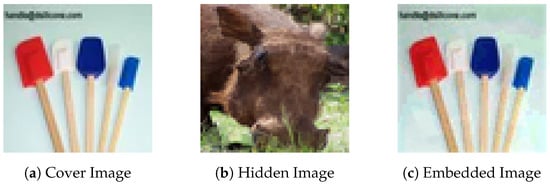
Figure 1. Vague Outline Visible in 4-bit LSB Steganography Embedded-Cover-Diversity = 50%, Hidden-Decoded-Diversity = 50%, Payload Capacity = 12 bpp.

Some traditional steganography methods with balanced attributes are hiding information in the JPEG DCT components. For instance, A. Almohammad’s work [3] provides around 20% of payload capacity (based on the patterns) and still remains undetected through statistical analysis.

Most secure traditional image steganography methods recently have adopted several functions to evaluate the embedding localizations in the image, which enables content-adaptive steganography. HuGO [4] defines a distortion function domain by giving every pixel a changing cost or embedding impact based on its effect. It uses a weighted norm to represent the feature space. WOW (Wavelet Obtained Weights) [5] embeds information according to the textural complexity of the image regions. Work [6,7] have discussed some general ways of content-adaptive steganography to avoid statistical analysis. Work [8] is focusing on content-adaptive batched steganography. These methods highly depend on the patterns of the cover image, and therefore the average payload capacity can be hard to calculate.

The major contributions of our work are as follows: (i) We propose a methodology to apply neural networks for image steganography to embed image information into image information without any help of traditional steganography methods; (ii) Our implementation raises image steganography payload capacity to an average of 98.2% or 23.57 bpp (bits per pixel), changing only around 0.76% of the cover image (See Figure 2); (iii) We propose a new cost function named variance loss to suppress noise pixels generated by generator network; (iv) Our implementation is robust to statistical analysis and 4 other widely used steganography analysis methods.

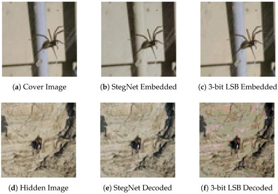
Figure 2. StegNet and 3-bit LSB Comparison Embedded-Cover-Diversity = 0.76%, Hidden-Decoded- Diversity = 1.8%, Payload Capacity = 23.57 bpp.

The decoded rate is calculated by

$$\mathrm{Decoded}\mathrm{Rate}=1-\frac{{\sum }_{i=1}^N{\sum }_{j=1}^M\left|H_{i,j}-D_{i,j}\right|}{N\times M},$$

(1)

the cover changing rate is calculated by

$$\mathrm{Cover}\mathrm{Changing}\mathrm{Rate}=\frac{{\sum }_{i=1}^N{\sum }_{j=1}^M\left|C_{i,j}-E_{i,j}\right|}{N\times M}$$

(2)

and the bpp (bits per pixel) is calculated by

$$\mathrm{Capacity}=\mathrm{Decoded}\mathrm{Rate}\times 8\times 3\left(\mathrm{bpp}\right)$$

(3)

where $C,H,E,D$ symbols stand for the cover image (C), the hidden image (H), the embedded image (E) and the decoded image (D) in correspondence, and “8, 3” stands for number of bits per channel and number of channels per pixel respectively.

This paper is organized as follows. Section 2 will describe traditional high-capacity steganography methods and the convolution neural network used by this paper. Section 3 will unveil the secret why the neural network can achieve the amount of capacity encoding and decoding images. The architecture and experiments of our neural network are discussed in Section 4 and Section 5, and finally, we’ll make a conclusion and put forward some future works in Section 6.

2. Related Work

2.1. Steganography Methods

Most steganography methods can be grouped into three basic types, which is image domain steganography, transform domain steganography and file-format-based steganography. Image domain ones have an advantage of simplicity and better payload capacity while being more likely to be detected. Transform domain ones usually have a more complex algorithm but hides pretty well through third-party analysis. File-format-based ones depend very much on the file format which makes it quite fragile to alterations.

2.2. JPEG RAR Steganography

The JPEG RAR Steganography is a kind of file-format-based steganography, which uses a feature in these two file format specifications (JPEG [9] and RAR [10]).

After the JPEG file has scanned the segment of EOI (End Of Image) (0xd9 in hex format), all the remaining segments are ignored (skipped), and therefore any information is allowed to be appended afterward. A RAR file [10] has the magic file header “0x52 0x61 0x72 0x21 0x1a 0x07 0x00” in hex format (“Rar!” as characters) and the parser will ignore all the information before the file header. It is possible to dump the binary of the RAR file after the JPEG file, and it’ll apparently act as if it is a JPEG image file while it is actually also a RAR archive. However, the method is very fragile to any file alterations. Third-party surveillance might truncate useless information to save transmission resource or apply some image alterations to attack potential steganography. Any alteration will crash the steganography, and all hidden information is lost.

2.3. LSB (Least Significant Bit) Method

LSB (Least Significant Bit)-based methods [1] are the most commonly used image domain steganography methods which hide information at the pixel level. Most LSB methods aim at altering parts of the cover image to such an extent that human visual system can barely notice. These methods are motivated by the fact that the visual part of most figures is dominated by the highest bits of each pixel, and the LSB bits (the underlined part of one pixel as shown in Figure 3) are statistically similar to randomly generated data, and therefore, hiding information via altering LSB cannot change the visual result apparently.

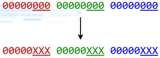
Figure 3. LSB Explaination.

The embedding operation of LSB method for the least bit single channel image is described as follows:

$$S_i=(C_i\wedge {\mathrm{FE}}_{\mathrm{HEX}})\vee ((M_i\wedge {80}_{\mathrm{HEX}})>>7)$$

where $S_i$, $C_i$ and $M_i$ are the ith pixel of image after steganography, ith pixel of cover image and ith bit of the hiding message.

Since the least significant bits of the image data should look like random data, there are major two schemes in distributing the hiding data. The first kind of methods is to put in the hiding message sequentially after encrypting or compressing to achieve the randomness. The second kind of methods is scattering the hiding data by adopting a mutually acknowledged random seed by which generates the actual hiding sequence [11].

2.4. JPEG Steganography

JPEG steganography, i.e., Chang’s work [12] and A. Almohammad’s work [3], is a part of transform domain steganography. JPEG format examines an image in $8\times 8$ blocks of pixels, converts from RGB color space into YCrCb (luminance and chrominance) color space, applies DCT (Discrete Cosine Transformation), quantizes the result, and entropy encodes the rest. After lossy compression, which is after quantization, the hidden information is hidden into the quantized DCT components, which serves as an LSB embedding in the transformed domain. As a result, it is quite hard to detect using statistical analysis and comparably lower payload capacity to LSB method.

2.5. Convolutional Neural Network

Convolutional neural network [13], though dates back to the 1990s, is now trending these years after AlexNet [14] won the championship of ImageNet competition. It has successfully established new records in many fields like classification [15], object segmentation [16], etc. A lot of factors boosted the progress including the development of modern GPU hardware, the work of ReLU (Rectified Linear Unit) [17] and its extensions, and finally, the abundance of training data [18]. Our work also benefits a lot from these factors.

The convolution operation is not solely used in neural networks, but also widely used in traditional computer vision methods. For instance, gaussian smoothing kernel is extensively used for image blurring and noise reduction, which, in implementation, is equal to applying a convolution between the original image and a gaussian function. Many other contributions in traditional methods are handcrafted patterns, kernels or filter combinations, i.e., the Sobel-Feldman filter [19] for edge detection, Log-Gabol filter [20] for texture detection, HOG [21] for object detection, etc.

However, designing and tuning handcrafted patterns are highly technical and might be effective for only some tasks. On the contrary, convolutional neural networks have the advantage of automatically creating patterns for specific tasks through back-propagation [22] on its own, and even further, high-level features can be easily learned through combinations of convolution operations [23,24,25].

2.6. Autoencoder Neural Network

Our method is inspired by traditional autoencoder neural networks [26], which was originally trained to generate an output image the same as input image in appearance. It is usually made up of two neural networks, one encoding network $h=f\left(x\right)$ and one decoding network $d=g\left(h\right)$, restricted under $d=x$, who finally can learn the conditional probability distribution of $p\left(h\right|x)$ and $p\left(x\right|h)$ correspondently. The autoencoder architecture has shown the ability to extract salient features in from images seen through shrinking hidden layer (h)’s dimension, which has been applied to various fields, i.e., denoising [27], dimension reduction [28], image generation [29], etc.

2.7. Neural Network for Steganography

Recently there are some works on applying neural networks for steganography. El-Emam [30] and Saleema [31] work on using neural networks to refine the embedded image generated via traditional steganography methods, i.e., LSB method. Volkhonskiy’s [32] and Shi’s [33] work focus on generating secure cover images for traditional steganography methods to apply image steganography. Baluja [34] is working on the same field as StegNet. However, the hidden image is slightly visible on residual images of the generated embedded images. Moreover, his architecture uses three networks which requires much more GPU memory and takes more time to embed.

3. Convolutional Neural Network for Image Steganography

3.1. High-order Transformation

In image steganography, we argue that we should not only focus on where to hide information, which most traditional methods work on, but we should also focus on how to hide it.

Most traditional steganography methods usually directly embed hidden information into parts of pixels or transformed correspondances. The transformation regularly occurs in where to hide, either actively applied in the steganography method or passively applied because of file format. As a result, the payload capacity is highly related and restricted to the area of the texture-rich part of the image detected by the handcoded patterns.

DCT-based steganography is one of the most famous transform domain steganography. We can consider the DCT process in JPEG lossy compression process as a kind of one-level high-order transformation which works at a block level, converting each $8\times 8$ or $16\times 16$ block of pixel information into its corresponding frequency-domain representation. Even hiding in DCT transformed frequency-domain data, traditional works [3,12] embed hidden information in mid-frequency band via LSB-alike methods, which eventually cannot be eluded.

While in contrast, deep convolution neural network makes multi-level high-order transformations possible for image steganography. Figure 4 shows the receptive field of one high-level kernel unit in a demo of a three-layer convolutional neural network. After lower-level features are processed by kernels and propagated through activations along middle layers, the receptive field of final higher-level kernel unit is able to absorb 5 lower-level features of the first layer and form its own higher-level feature throughout the training process.

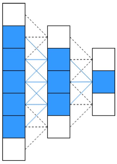
Figure 4. Receptive Field of Convolutional Neural Network.

3.2. Trading Accuracy for Capacity

Traditional image steganography algorithms mostly embed hidden information as it is or after applying lossless transformations. After decoding, the hidden information is extracted as it is or after the corresponding detransformations are applied. Therefore, empirically speaking, it is just as file compression methods, where lossless compression algorithms usually cannot outperform lossy compression algorithms in capacity.

We need to think in a “lossy” way in order to embed almost equal amount of information into the cover. The model needs to learn to compress the cover image and the hidden image into an embedding of high-level features and converts them into an image that appears as similar as the cover image, which comes to the vital idea of trading accuracy for capacity.

Trading accuracy for capacity means that we do not limit our model in reconstructing at a pixel-level accuracy of the hidden image, but aiming at “recreating” a new image with most of the features in it with a panoramic view, i.e., the spider in the picture, the pipes’ position relatively correct, the outline of the mountain, etc.

In other words, the traditional approaches work in lossless ways, which after some preprocessing to the hidden image, the transformed data is crammed into the holes prepared in the cover image. However, StegNet approach decoded image has no pixel-wise relationship with the hidden image at all, or strictly speaking, there is no reasonable transformation between each pair of corresponding pixels, but the decoded image as a whole can represent the original hidden image’s meaning through neural network’s reconstruction.

In the encoding process, the model needs to transform from a low-level massive amount of pixel-wise information into some high-level limited sets of featurewise information with an understanding of the figure, and come up with a brand new image similar to the cover apparently but with hidden features embedded. In the decoding process, on the contrary, the model is shown only the embedded figure, from which both cover and hidden high-level features are extracted, and the hidden image is rebuilt according to network’s own comprehension.

As shown in Figure 5 and Figure 6, StegNet is not applying LSB-like or simple merging methods to embed the hidden information into the cover. The residual image is neither simulating random noise (LSB-based approach, see Figure 7) nor combining recognizable hidden image inside. The embedded pattern is distributed across the whole image and even magnified 5 to 10 times, the residual image is similar to the cover image visually which can help decrease the abnormality exposed to the human visual system and finally avoid to be detected.

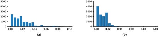
Figure 5. Residual image histograms shows that the residual error is distributed across the images. (a) Residual between cover and embedded; (b) Residual between hidden and decoded.

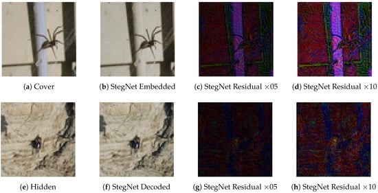
Figure 6. StegNet residual images “$\times 05$” and “$\times 10$” are the pixel-wise enhancement ratio.

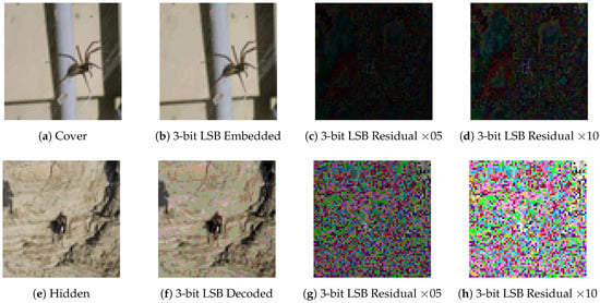
Figure 7. 3-bit LSB residual images “$\times 05$” and “$\times 10$” are the pixel-wise enhancement ratio.

The residual image is computed via

$$R(I_1,I_2)=\frac{\left|I_1-I_2\right|}{max\left|I_1-I_2\right|},$$

(4)

and the magnification or the enhancement operation is achieved via

$$E(I,M)=\mathrm{clip}(I·M,0,1),$$

(5)

where I takes residual images, which are effectively normalized to $[0,1]$ and M is the magnification ratio, which 5 and 10 are chosen visualize the differences in this paper.

4. Architecture

4.1. Architecture Pipeline

The whole processing pipeline is shown in Figure 8, which consists of two almost identical neural network structure responsible for encoding and decoding. The identical structures are taken from Autoencoder [26], GAN [35], etc., which help the neural network model similar high-level features of images in their latent space. The details of embedding and decoding structure are described in Figure 9. In the embedding procedure, the cover image and the hidden image are concatenated by channel while only the embedded image is shown to the network. Two parts of the network are both majorly made up of one lifting layer which lifts from figure channels to a uniform of 32 channels, six $3\times 3$ basic building blocks raising features into high-dimensional latent space and one reducing layer which transforms features back to image space.

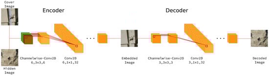
Figure 8. StegNet Processing Pipeline.

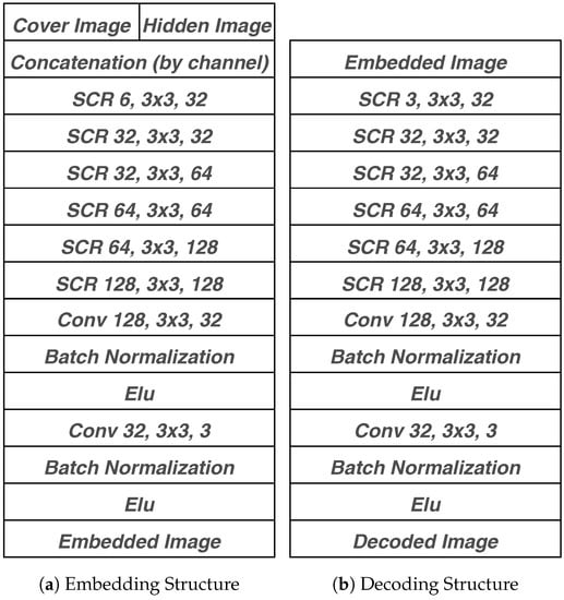
Figure 9. StegNet Network Architecture.

The basic building block named “Separable Convolution with Residual Block” (abbreviated as “SCR” in the following context) has the architecture as Figure 10. We adopt batch-normalization [36] and exponential linear unit (ELU) [37] for quicker convergence and better result.

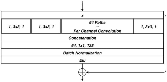
Figure 10. Separable Convolution with Residual Block.

4.2. Separable Convolution with Residual Block

Our work adopt the state of the art neural network structure, the skip connections in Highway Network [38], ResNet [39] and ResNeXt [40], and separable convolution [41] together to form the basic building block “SCR”.

The idea behind separable convolution [41] originated from Google’s Inception models [42,43] (see Figure 11 for its building blocks), and the hypothesis behind is that “cross-channel correlations and spatial correlations are decoupled”. Further, in Xception architecture [41], it makes an even stronger hypothesis that “cross-channel correlations and spatial correlations can be mapped completely separately”. Together with skip-connections [39] the gradients are preserved in backpropagation process via skip-connections to frontier layers and as a result, ease the problem of vanishing gradients.

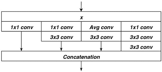
Figure 11. Basic Building Block in Inception v3.

4.3. Training

Learning the end-to-end mapping function from cover and hidden image to embedded image and embedded image to decoded image requires the estimation of millions of parameters in the neural network. It is achieved via minimizing the weighted loss of $L_1$-loss between the cover and the embedded image, $L_1$-loss between the hidden and the decoded image, and their corresponding variance losses (variance should be computed across images’ height, width and channel). $C,H,E,D$ symbols stand for the cover image (C), the hidden image (H), the embedded image (E) and the decoded image (D) in correspondence (See Equations (6)–(8)).

$$\begin{array}{cccc}\hfill E_i& =F_{\mathrm{CE}}(C_i,H_i;{\mathsf{\Theta }}_{\mathrm{CE}})\hfill & \hfill D_i& =F_{\mathrm{ED}}(E_i;{\mathsf{\Theta }}_{\mathrm{ED}})\hfill \end{array}$$

(6)

$$\begin{array}{cccc}\hfill L_{\mathrm{CE}}& =\frac{1}{n}\sum _{i=1}^n\left|E_i-C_i\right|\hfill & \hfill L_{\mathrm{HD}}& =\frac{1}{n}\sum _{i=1}^n\left|D_i-H_i\right|\hfill \end{array}$$

(7)

$$\mathrm{Loss}=\frac{1}{4}(L_{\mathrm{CE}}+L_{\mathrm{HD}}+\mathrm{Var}\left(L_{\mathrm{CE}}\right)+\mathrm{Var}\left(L_{\mathrm{HD}}\right))$$

(8)

$L_{\mathrm{CE}}$ is used to minimize the difference between the embedded image and the cover image, while $L_{\mathrm{HD}}$ is for the hidden image and the decoded image. Choosing only to decode the hidden image while not both the cover and the hidden images are under the consideration that the embedded image should be a concentration of high-level features apparently similar to the cover image whose dimension is half the shape of those two images, and some trivial information has been lost. It would have pushed the neural network to balance the capacity in embedding the cover and the hidden if both images are extracted at the decoding process.

Furthermore, adopting variance losses helps to give a hint to the neural network that the loss should be distributed throughout the image, but not putting at some specific position (See Figure 12 for differences between. The embedded image without variance loss shows some obvious noise spikes (blue points) in the background and also some around the dog nose).

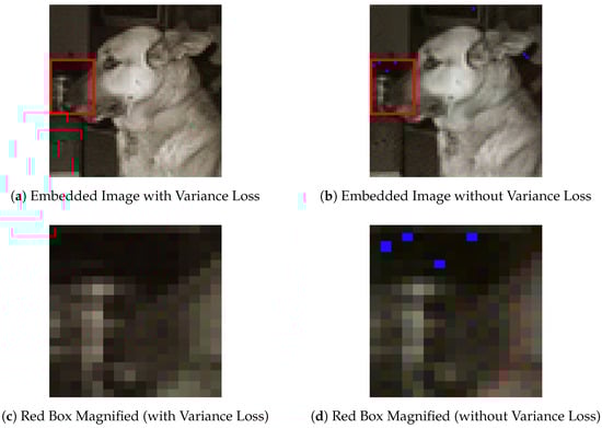
Figure 12. Variance Loss Effect on Embedding Results.

5. Experiments

5.1. Environment

Our work is trained on one NVidia GTX1080 GPU and we adopt a batch size of 64 using Adam optimizer [44] with learning rate at ${10}^{-5}$. We use no image augmentation and restrict model’s input image to $64\times 64$ in height and width because of memory limit. Training with resized $64\times 64$ ImageNet can yield pretty good results. We use 80% of the ImageNet dataset for training and the remaining for testing to verify the generalization ability of our model. Figure 13 shows the result of applying StegNet steganography method on a batch of images.

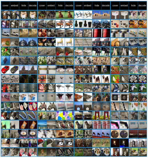
Figure 13. One batch Steganography Example.

5.2. Statistical Analysis

The encoded and decoded images comparison between StegNet and LSB method are presented in Figure 2. They are very similar though, however, there is one critical flaw about the LSB method, in that it does not suffer through statistical analysis, and therefore LSB method is usually combined with transformations of the hidden image, i.e., compression, randomization, etc.

Figure 14 is a comparison of histogram analysis between LSB method and our work. It shows a direct view of robustness of StegNet against statistical analysis, which the StegNet embedded’s histogram and the cover image’s histogram are much more matching.

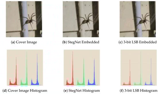
Figure 14. Histogram Comparison between StegNet and Plain LSB.

A more all-around test is conducted through StegExpose [45], which combines several decent algorithms to detect LSB-based steganography, i.e., sample pair analysis [46], RS analysis [47], chi-square attack [48] and primary sets [49]. The detection threshold is its hyperparameter, which is used to balance true positive rate and false positive rate of the StegExpose’s result. The test is performed with linear interpolation of detection threshold from 0.00 to 1.00 with 0.01 as the step interval.

Figure 15 is the ROC curve, where true positive stands for an embedded image correctly identified that there are hidden data inside while false positive means a clean figure falsely classified as an embedded image. The figure is plotted in red-dash-line-connected scatter data, showing that StegExpose can only work a little better than random guessing, the line in green. In other words, the proposed steganography method can better resist StegExpose attack.

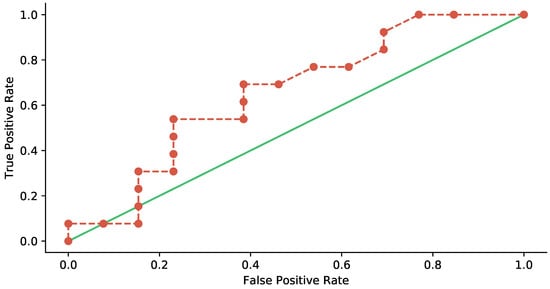
Figure 15. ROC Curves: Detecting Steganography via StegExpose.

6. Conclusions and Future Work

We have presented a novel deep learning approach for image steganography. We show that the conventional image steganography methods mostly do not serve with good payload capacity. The proposed approach, StegNet, creates an end-to-end mapping from the cover image, hidden image to embedded image and from embedded image to decoded image. It has achieved superior performance than traditional methods and yet remains quite robust.

As seen in Figure 13, there is still some noise generated at non-texture-rich areas, i.e., plain white or plain black parts. The variance loss adopted by StegNet might not be the optimal solution to loss distribution.

In addition to the idea of “trading accuracy for capacity”, the embedded image does not need to be even visually similar to the cover image. The only requirement to the embedded image is to pass the third-party supervision and the hidden image should be successfully decoded after the transmission is complete, and therefore the embedded image can look similar to anything that is inside the cover image dataset while can look nothing related to anything that is inside the hidden image dataset. Some of the state of the art generative models in neural networks can help achieve it, i.e., Variational Autoencoders [29,50], Generative Adversarial Networks [35,51,52], etc.

Some work is needed for non-equal sized images steganography since “1:1” image steganography is huge for traditional judgment; however, the ability of neural networks still remains to be discovered. Whether it is possible to generate approaches for even better capacity, or with a better visual quality for even safer from detections. Some other work is needed for non-image hidden information steganography, i.e., text information, binary data. In addition to changing the hidden information type, the cover information type may also vary from text information to even videos. Furthermore, some work is needed for applying StegNet on lossy-compressed image file formats or third-party spatial translations, i.e., cropping, resizing, stretching, etc.

References

- Mielikainen, J. Lsb matching revisited. IEEE Signal Process. Lett. 2006, 13, 285–287. [Google Scholar] [CrossRef]
- Kawaguchi, E.; Eason, R. Principle and applications of BPCS-Steganography. In Proceedings of the SPIE 3528, Multimedia Systems and Applications, Boston, MA, USA, 22 January 1999. [Google Scholar]
- Almohammad, A.; Hierons, R.M.; Ghinea, G. High Capacity Steganographic Method Based Upon JPEG. In Proceedings of the Third International Conference on Availability, Reliability and Security, Barcelona, Spain, 4–7 March 2008. [Google Scholar]
- Pevný, T.; Filler, T.; Bas, P. Using High-Dimensional Image Models to Perform Highly Undetectable Steganography. In Information Hiding; Lecture Notes in Computer Science; Springer: Berlin/Heidelberg, Germany, 2010; pp. 161–177. [Google Scholar]
- Holub, V.; Fridrich, J. Designing steganographic distortion using directional filters. In Proceedings of the 2012 IEEE International Workshop on Information Forensics and Security (WIFS), Tenerife, Spain, 2–5 December 2012; pp. 234–239. [Google Scholar]
- Holub, V.; Fridrich, J.; Denemark, T. Universal distortion function for steganography in an arbitrary domain. EURASIP J. Inf. Secur. 2014, 2014. [Google Scholar] [CrossRef]
- Sedighi, V.; Cogranne, R.; Fridrich, J. Content-Adaptive Steganography by Minimizing Statistical Detectability. IEEE Trans. Inf. Forensics Secur. 2016, 11, 221–234. [Google Scholar] [CrossRef]
- Cogranne, R.; Sedighi, V.; Fridrich, J. Practical strategies for content-adaptive batch steganography and pooled steganalysis. In Proceedings of the 2017 IEEE International Conference on Acoustics, Speech and Signal Processing (ICASSP), New Orleans, LA, USA, 5–9 March 2017; pp. 2122–2126. [Google Scholar]
- Digital Compression and Coding of Continuous-Tone Still Images: Requirements and Guidelines; Technical Report ISO/IEC 10918-1:1994; Joint Photographic Experts Group Committee: La Jolla, CA, USA, 1994.
- Roshal, A. RAR 5.0 Archive Format. 2017. Available online: https://www.rarlab.com/technote.htm (accessed on 5 October 2017).
- Juneja, M.; Sandhu, P. Designing of robust image steganography technique based on LSB insertion and encryption. In Proceedings of the IEEE International Conference on Advances in Recent Technologies in Communication and Computing, Kerala, India, 27–28 October 2009; pp. 302–305. [Google Scholar]
- Chang, C.C.; Chen, T.S.; Chung, L.Z. A steganographic method based upon JPEG and quantization table modification. Inf. Sci. 2002, 141, 123–138. [Google Scholar] [CrossRef]
- Lecun, Y.; Boser, B.; Denker, J.S.; Henderson, D.; Howard, R.E.; Hubbard, W.; Jackel, L.D. Backpropagation applied to hand-written zip code recognition. Neural Comput. 1989, 1, 541–551. [Google Scholar] [CrossRef]
- Krizhevsky, A.; Sutskever, I.; Hinton, G.E. Imagenet classification with deep convolutional neural networks. In Proceedings of the 25th International Conference on Neural Information Processing Systems, Lake Tahoe, NV, USA, 3–6 December 2012; pp. 1097–1105. [Google Scholar]
- Hu, J.; Shen, L.; Sun, G. Squeeze-and-Excitation Networks. arXiv, 2017; arXiv:1709.01507. [Google Scholar]
- Li, Y.; Qi, H.; Dai, J.; Ji, X.; Wei, Y. Fully Convolutional Instance-aware Semantic Segmentation. arXiv, 2017; arXiv:1611.07709. [Google Scholar]
- Nair, V.; Hinton, G.E. Rectified linear units improve restricted Bolzmann machines. In Proceedings of the 27th International Conference on Machine Learning, Haifa, Israel, 21–24 June 2010; Volume 27, pp. 807–814. [Google Scholar]
- Deng, J.; Dong, W.; Socher, R.; Li, L.J.; Li, K.; Fei-Fei, L. ImageNet: A Large-Scale Hierarchical Image Database. In Proceedings of the IEEE Conference on Computer Vision and Pattern Recognition, Miami, FL, USA, 20–25 June 2009. [Google Scholar]
- Sobel, I.; Feldman, G. An Isotropic 3 × 3 Image Gradient Operator. In Pattern Classification and Scene Analysis; Wiley: Hoboken, NJ, USA, 1973; pp. 271–272. [Google Scholar]
- Fischer, S.; Sroubek, F.; Perrinet, L.U.; Redondo, R.; Cristóbal, G. Self-invertible 2D log-Gabor wavelets. Int. J. Comput. Vis. 2007, 75, 231–246. [Google Scholar] [CrossRef]
- Dalal, N.; Triggs, B. Histograms of oriented gradients for human detection. In Proceedings of the IEEE Computer Society Conference on Computer Vision and Pattern Recognition, San Diego, CA, USA, 20–25 June 2005; Volume 1, pp. 886–893. [Google Scholar]
- Rumelhart, D.E.; Hinton, G.E.; Williams, R.J. Learning representations by back-propagating errors. Nature 1986, 323, 533. [Google Scholar] [CrossRef]
- Zeiler, M.D.; Fergus, R. Visualizing and Understanding Convolutional Networks. In Proceedings of the Computer Vision—ECCV 2014, Zurich, Switzerland, 6–12 September 2014; Volume 8689, pp. 818–833. [Google Scholar] [CrossRef]
- Olah, C.; Mordvintsev, A.; Schubert, L. Feature Visualization. Distill 2017. [Google Scholar] [CrossRef]
- Mahendran, A.; Vedaldi, A. Understanding Deep Image Representations by Inverting Them. arXiv, 2015; arXiv:1412.0035. [Google Scholar]
- Hinton, G.E.; Zemel, R.S. Autoencoders, minimum description length and Helmholtz free energy. In Proceedings of the Advances in Neural Information Processing Systems, Denver, Colorado, 28 November–1 December 1994; pp. 3–10. [Google Scholar]
- Vincent, P.; Larochelle, H.; Bengio, Y.; Manzagol, P.A. Extracting and composing robust features with denoising autoencoders. In Proceedings of the 25th International Conference on Machine Learning, Helsinki, Finland, 5–9 July 2008; pp. 1096–1103. [Google Scholar]
- Wang, W.; Huang, Y.; Wang, Y.; Wang, L. Generalized autoencoder: A neural network framework for dimensionality reduction. In Proceedings of the IEEE Conference on Computer Vision and Pattern Recognition Workshops, Columbus, OH, USA, 23–28 June 2014; pp. 490–497. [Google Scholar]
- Kingma, D.P.; Welling, M. Auto-Encoding Variational Bayes. arXiv, 2013; arXiv:1312.6114. [Google Scholar]
- El-emam, N.N. Embedding a large amount of information using high secure neural based steganography algorithm. Int. J. Inf. Commun. Eng. 2008, 4, 223–232. [Google Scholar]
- Saleema, A.; Amarunnishad, T. A New Steganography Algorithm Using Hybrid Fuzzy Neural Networks. Procedia Technol. 2016, 24, 1566–1574. [Google Scholar] [CrossRef]
- Volkhonskiy, D.; Nazarov, I.; Borisenko, B.; Burnaev, E. Steganographic Generative Adversarial Networks. arXiv, 2017; arXiv:1703.05502. [Google Scholar]
- Shi, H.; Dong, J.; Wang, W.; Qian, Y.; Zhang, X. SSGAN: Secure Steganography Based on Generative Adversarial Networks. arXiv, 2017; arXiv:1707.01613. [Google Scholar]
- Baluja, S. Hiding Images in Plain Sight: Deep Steganograph. In Advances in Neural Information Processing Systems 30; Guyon, I., Luxburg, U.V., Bengio, S., Wallach, H., Fergus, R., Vishwanathan, S., Garnett, R., Eds.; Curran Associates, Inc.: Red Hook, NY, USA, 2017; pp. 2069–2079. [Google Scholar]
- Goodfellow, I.; Pouget-Abadie, J.; Mirza, M.; Xu, B.; Warde-Farley, D.; Ozair, S.; Courville, A.; Bengio, Y. Generative adversarial nets. In Proceedings of the Advances in neural information processing systems, Montreal, QC, Canada, 8–13 December 2014; pp. 2672–2680. [Google Scholar]
- Ioffe, S.; Szegedy, C. Batch Normalization: Accelerating Deep Network Training by Reducing Internal Covariate Shift. In Proceedings of the 32nd International Conference on International Conference on Machine Learning—Volume 37, Lille, France, 6–11 July 2015; pp. 448–456. [Google Scholar]
- Clevert, D.A.; Unterthiner, T.; Hochreiter, S. Fast and Accurate Deep Network Learning by Exponential Linear Units (ELUs). arXiv, 2015; arXiv:1511.07289. [Google Scholar]
- Srivastava, R.K.; Greff, K.; Schmidhuber, J. Highway Networks. arXiv, 2015; arXiv:1505.00387. [Google Scholar]
- He, K.; Zhang, X.; Ren, S.; Sun, J. Deep Residual Learning for Image Recognition. arXiv, 2016; arXiv:1512.03385. [Google Scholar]
- Xie, S.; Girshick, R.; Dollár, P.; Tu, Z.; He, K. Aggregated Residual Transformations for Deep Neural Networks. arXiv, 2017; arXiv:1611.05431. [Google Scholar]
- Chollet, F. Xception: Deep Learning with Depthwise Separable Convolutions. arXiv, 2016; arXiv:1610.02357. [Google Scholar]
- Szegedy, C.; Liu, W.; Jia, Y.; Sermanet, P.; Reed, S.; Anguelov, D.; Erhan, D.; Vanhoucke, V.; Rabinovich, A. Going deeper with convolutions. arXiv, 2015; arXiv:1409.4842. [Google Scholar]
- Szegedy, C.; Ioffe, S.; Vanhoucke, V.; Alemi, A.A. Inception-v4, inception-resnet and the impact of residual connections on learning. arXiv, 2017; arXiv:1602.07261. [Google Scholar]
- Kingma, D.; Ba, J. Adam: A Method for Stochastic Optimization. arXiv, 2014; arXiv:1412.6980. [Google Scholar]
- Boehm, B. StegExpose - A Tool for Detecting LSB Steganography. arXiv, 2014; arXiv:1410.6656. [Google Scholar]
- Dumitrescu, S.; Wu, X.; Wang, Z. Detection of LSB steganography via sample pair analysis. IEEE Trans. Signal Process. 2003, 51, 1995–2007. [Google Scholar] [CrossRef]
- Fridrich, J.; Goljan, M. Reliable Detection of LSB Steganography in Color and Grayscale Images. U.S. Patent 6,831,991, 14 December 2004. [Google Scholar]
- Westfeld, A.; Pfitzmann, A. Attacks on steganographic systems. In Proceedings of the International workshop on information hiding, Dresden, Germany, 29 September–1 October 1999; pp. 61–76. [Google Scholar]
- Dumitrescu, S.; Wu, X.; Memon, N. On steganalysis of random LSB embedding in continuous-tone images. In Proceedings of the 2002 International Conference on Image Processing, Rochester, NY, USA, 22–25 September 2002; Volume 3, pp. 641–644. [Google Scholar]
- Makhzani, A.; Shlens, J.; Jaitly, N.; Goodfellow, I. Adversarial Autoencoders. In Proceedings of the International Conference on Learning Representations, San Juan, Puerto Rico, 2–4 May 2016. [Google Scholar]
- Arjovsky, M.; Chintala, S.; Bottou, L. Wasserstein generative adversarial networks. In Proceedings of the International Conference on Machine Learning, Sydney, Australia, 6–8 August 2017; pp. 214–223. [Google Scholar]
- Berthelot, D.; Schumm, T.; Metz, L. BEGAN: Boundary Equilibrium Generative Adversarial Networks. arXiv, 2017; arXiv:1703.10717. [Google Scholar]
© 2018 by the authors. Licensee MDPI, Basel, Switzerland. This article is an open access article distributed under the terms and conditions of the Creative Commons Attribution (CC BY) license (http://creativecommons.org/licenses/by/4.0/).