Interest of a Full-Waveform Flown UV Lidar to Derive Forest Vertical Structures and Aboveground Carbon

Abstract
:1. Introduction
2. Instrumental Set-Up and Strategy
2.1. ULA Carrier

| Characteristics | Details |
|---|---|
| Maximal scientific payload | 120 kg |
| Flight speed | 17 to 40 m s−1 (62 to 144 km h−1) |
| Endurance | 4 h at 20 m s−1 (3 h at 40 m s−1) |
| Gross weight | 450 kg |
| Flight altitude | between 0.2 and 5.8 km agl |
| Climb rate | 6.5 m s−1 |
| Electric supply (2 × 12 V batteries) | 24 V/~400 W |
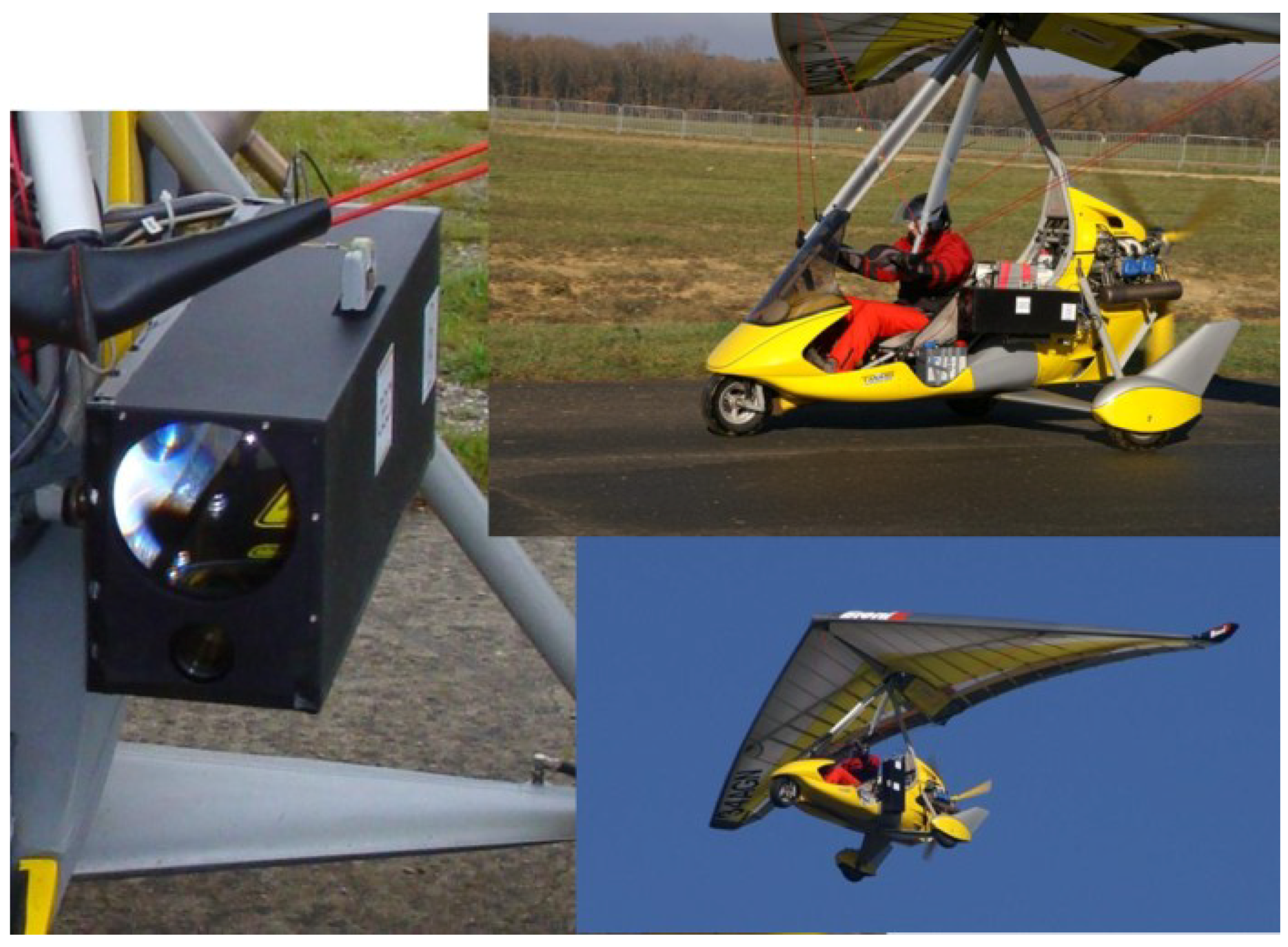
2.2. Scientific Payload
| Characteristics | Details |
|---|---|
| Wavelength | 355 nm |
| Mean energy per pulse | ~7 mJ |
| Pulse repetition frequency (PRF) | 1–100 Hz |
| Pulse duration | ~6 ns |
| Beam diameter | 20 mm |
| Diameter footprint at a flying altitude of 300 m agl | 2.20 m |
| Reception diameter | 150 mm |
| Reception optical density (OD) | 3.7 |
| Filter bandwidth | 0.3 nm |
| Field of view | ~4 mrad |
| Detector | Photomultiplicator |
| Detection mode | Analog |
| Vertical sampling | 0.75 m |
| Weight of the optical head | ~20 kg |
| Weight of the electronics | ~15 kg |
| Electric supply (2 × 12 V batteries) | 24 V/~400 W |
| Characteristics | Details |
|---|---|
| GPS | |
| Receiver type | 50 channels L1 frequency; C/A code Galileo L1; Open Service |
| GPS update rate | 4 Hz |
| Start-up time cold start | 29 s |
| Tracking sensitivity | −160 dBm |
| Timing accuracy | 50 ns RMS |
| AHRS | |
| Static accuracy (roll/pitch) | <0.5 deg |
| Static accuracy (heading) | <1 deg |
| Dynamic accuracy | 1 deg RMS |
| Angular resolution | 0.05 deg |
| Dynamic range: | |
| -Pitc | ±90 deg |
| -Roll/Heading | ±180 deg |
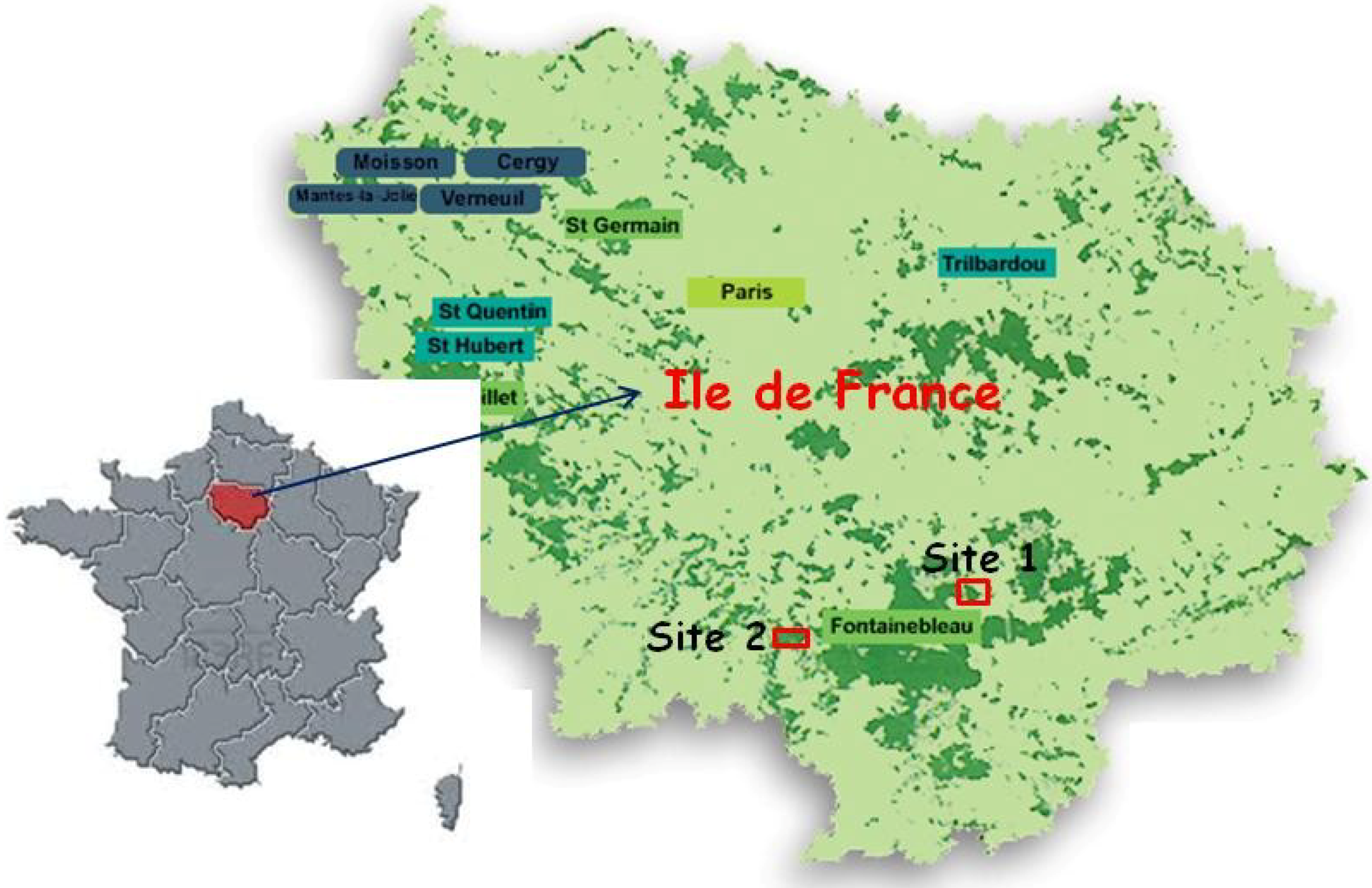
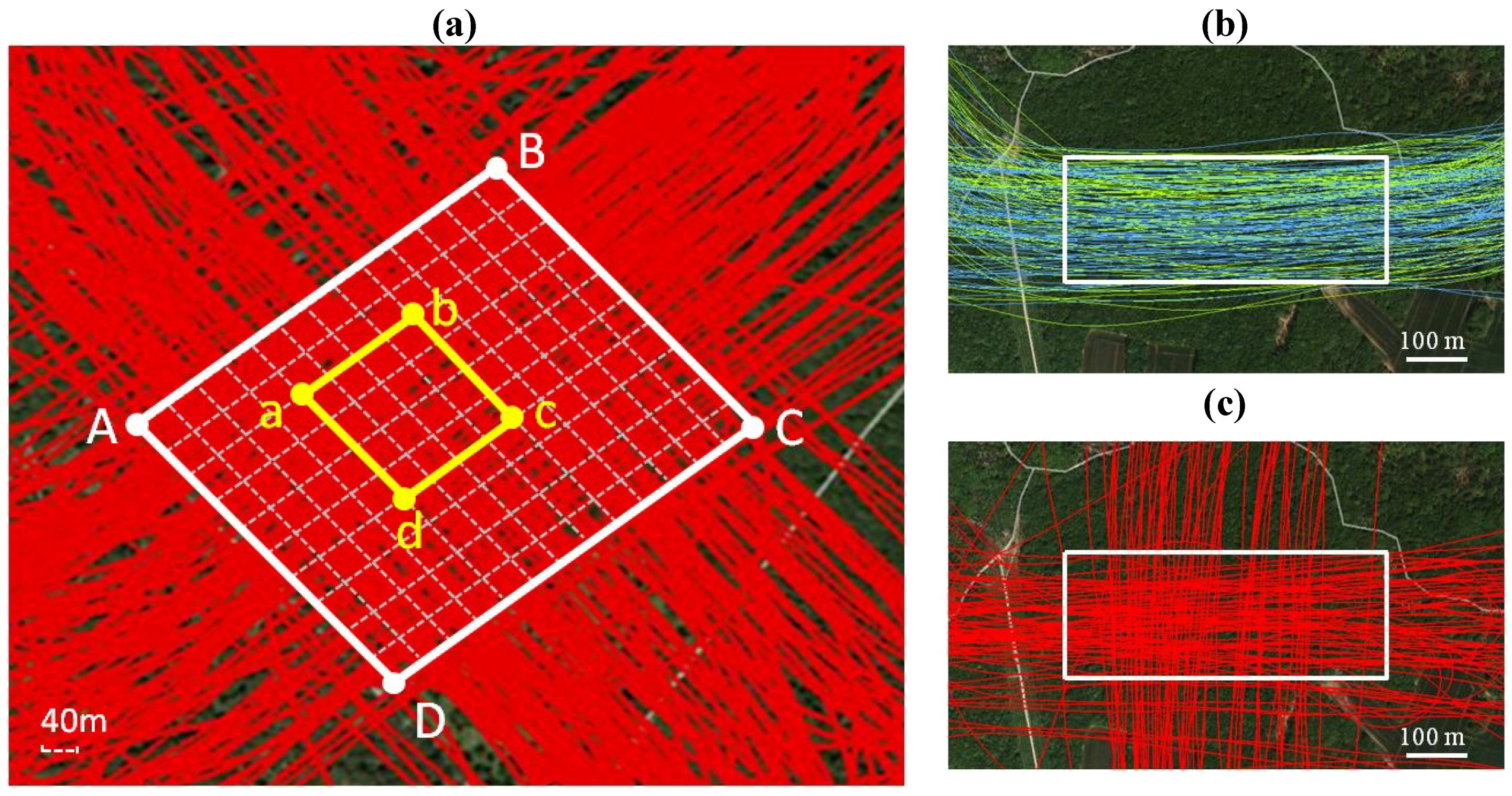
2.3. Forest Sites and Sampling Strategy

3. Theory
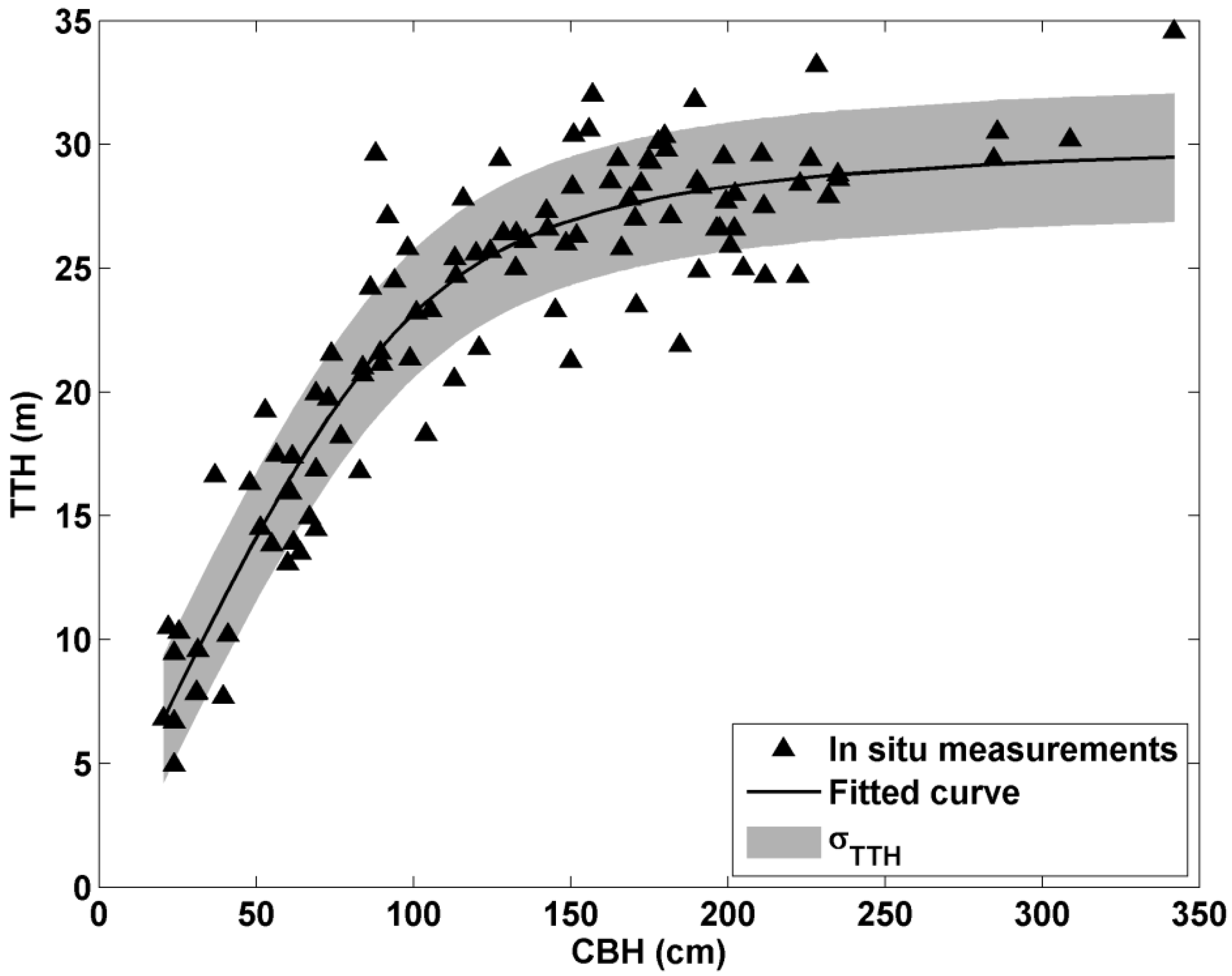
3.1. Tree Top Height (TTH) Retrieval from Lidar Measurements


 and
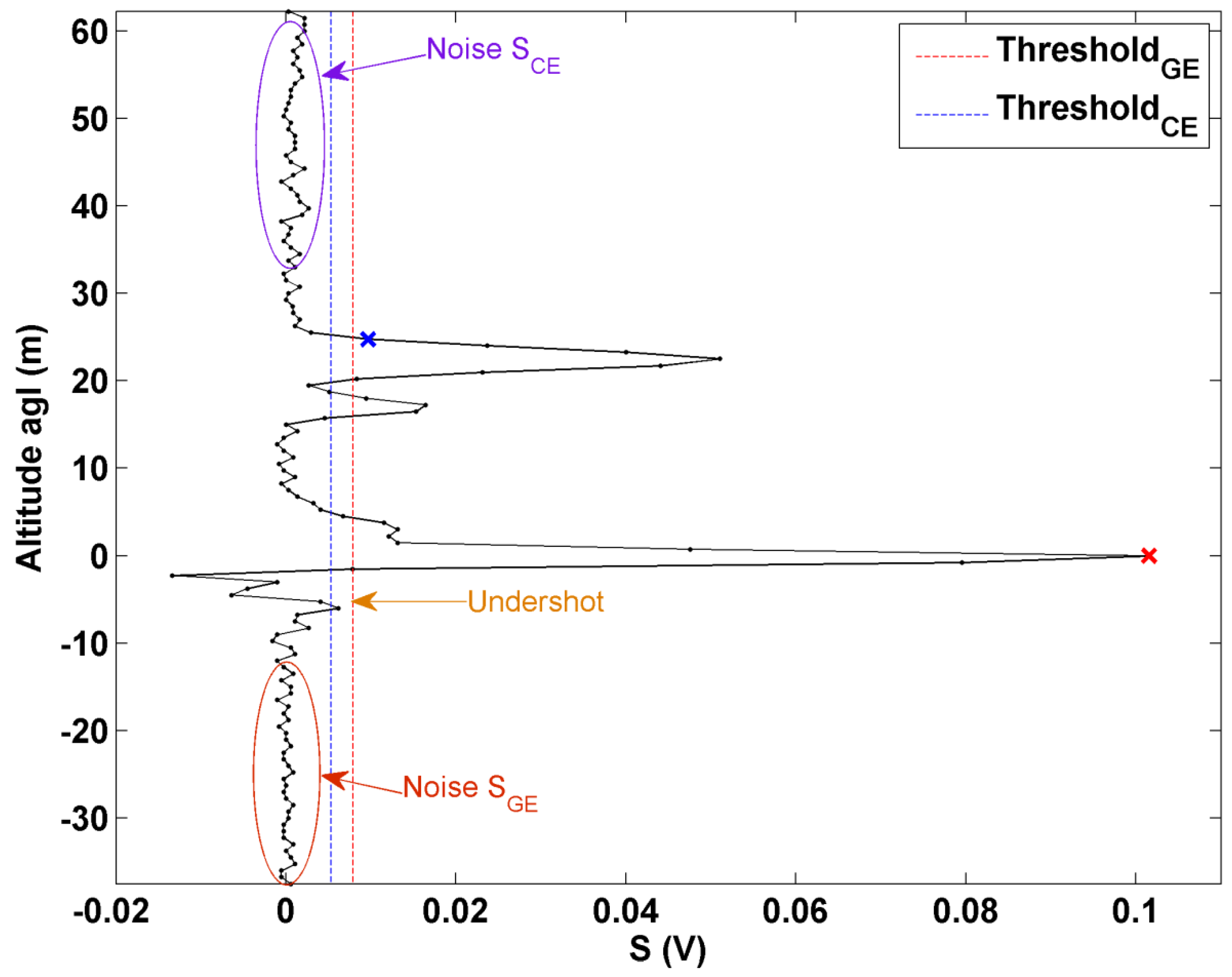
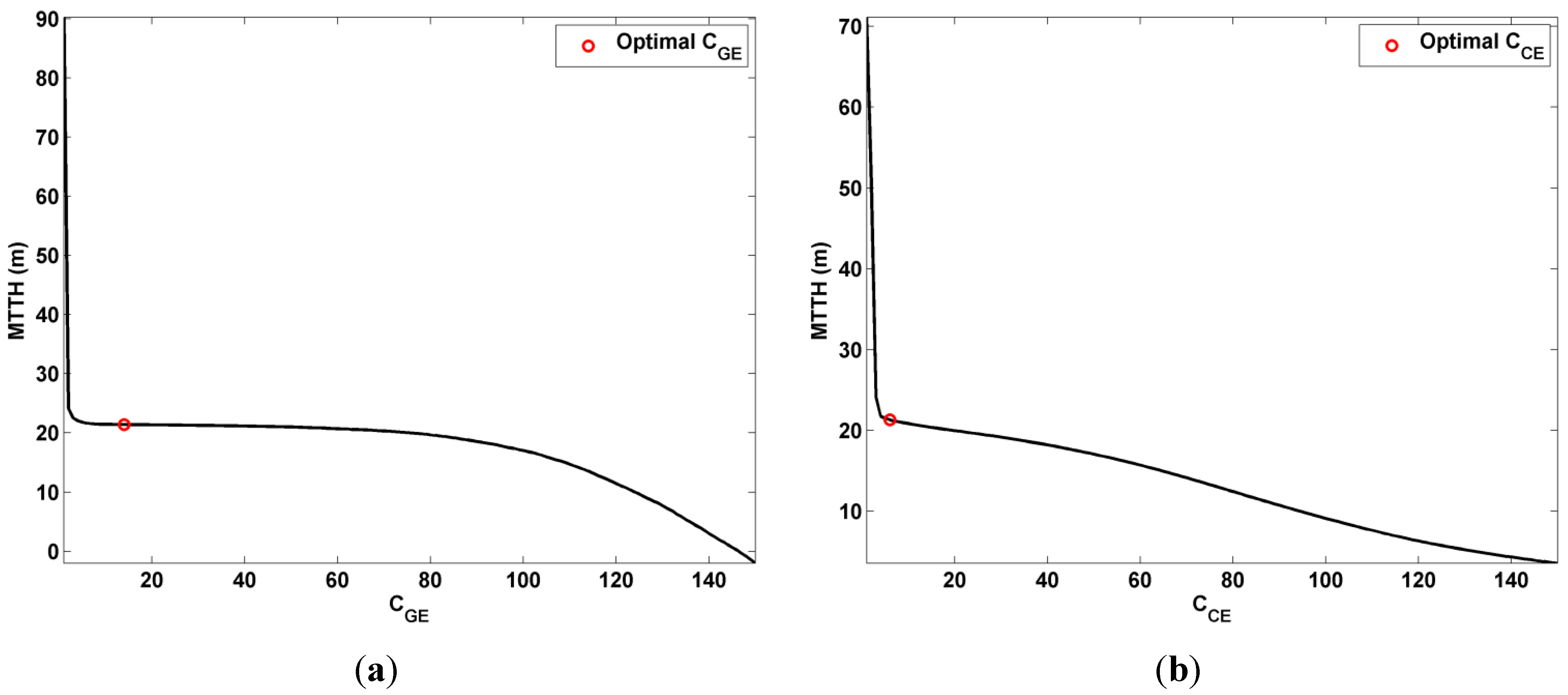
and  are the mean value and the standard deviation of SN (the noise signal), respectively, under the ground level for the GE (x = GE) and above the canopy top for the CE (x = CE). CGE and CCE are coefficients that are optimized by seeking the minimum relative residue on the mean tree top height (MTTH) retrieval following an iterative approach. Note that the lidar GE waveform should be calibrated by using the return laser pulse in the nadir/zenith direction over a flat surface such as the tarmac of the aerodrome from where the ULA took off.
3.2. Quadratic Mean Canopy Height (QMCH) Retrieval from Lidar Measurements


3.3. Aboveground Carbon (AGC) Retrieval from Field Measurements


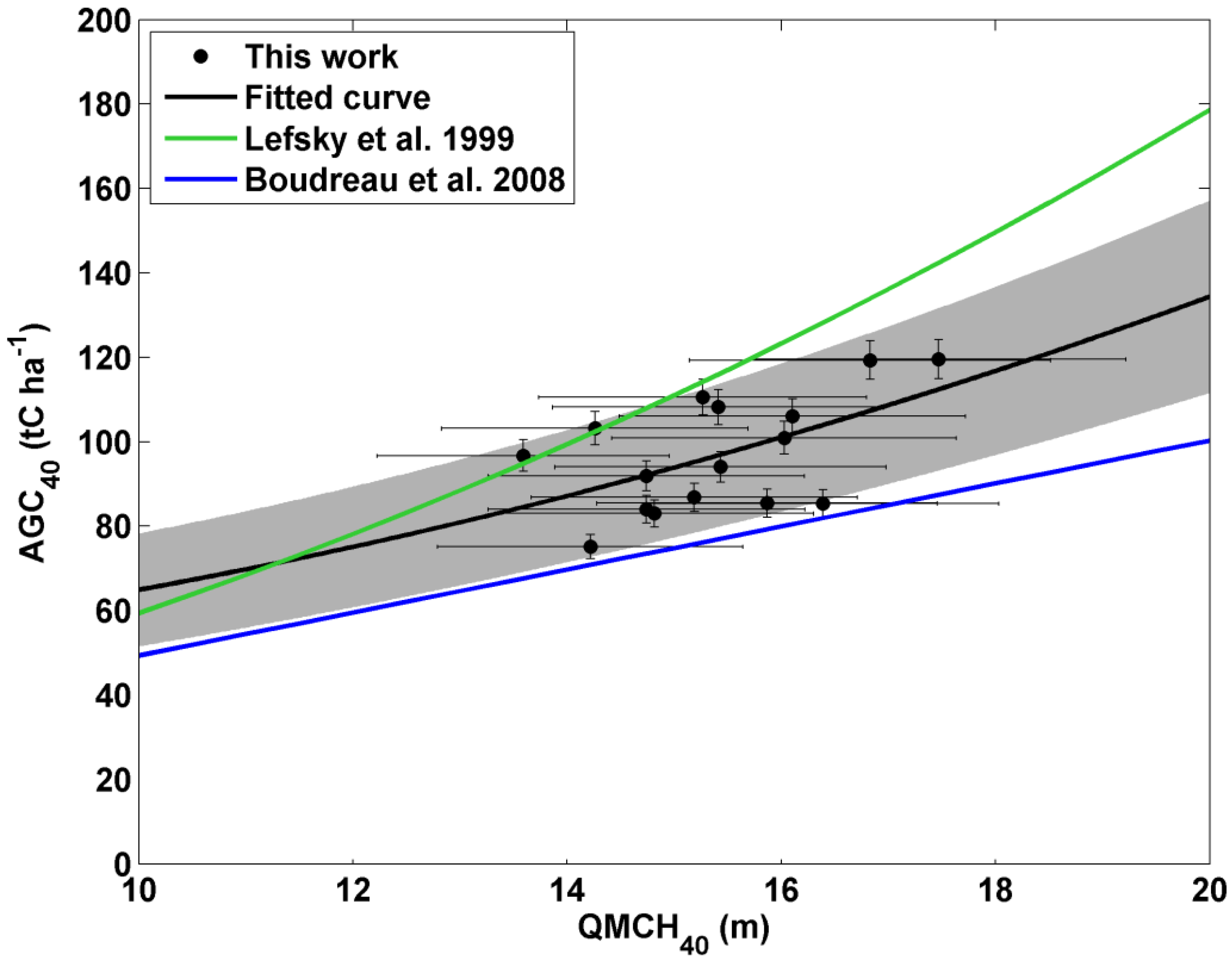
3.4. AGC Estimation via QMCH
4. Experimental Results and Uncertainties for Airborne Full-Waveform UV Lidar Measurements
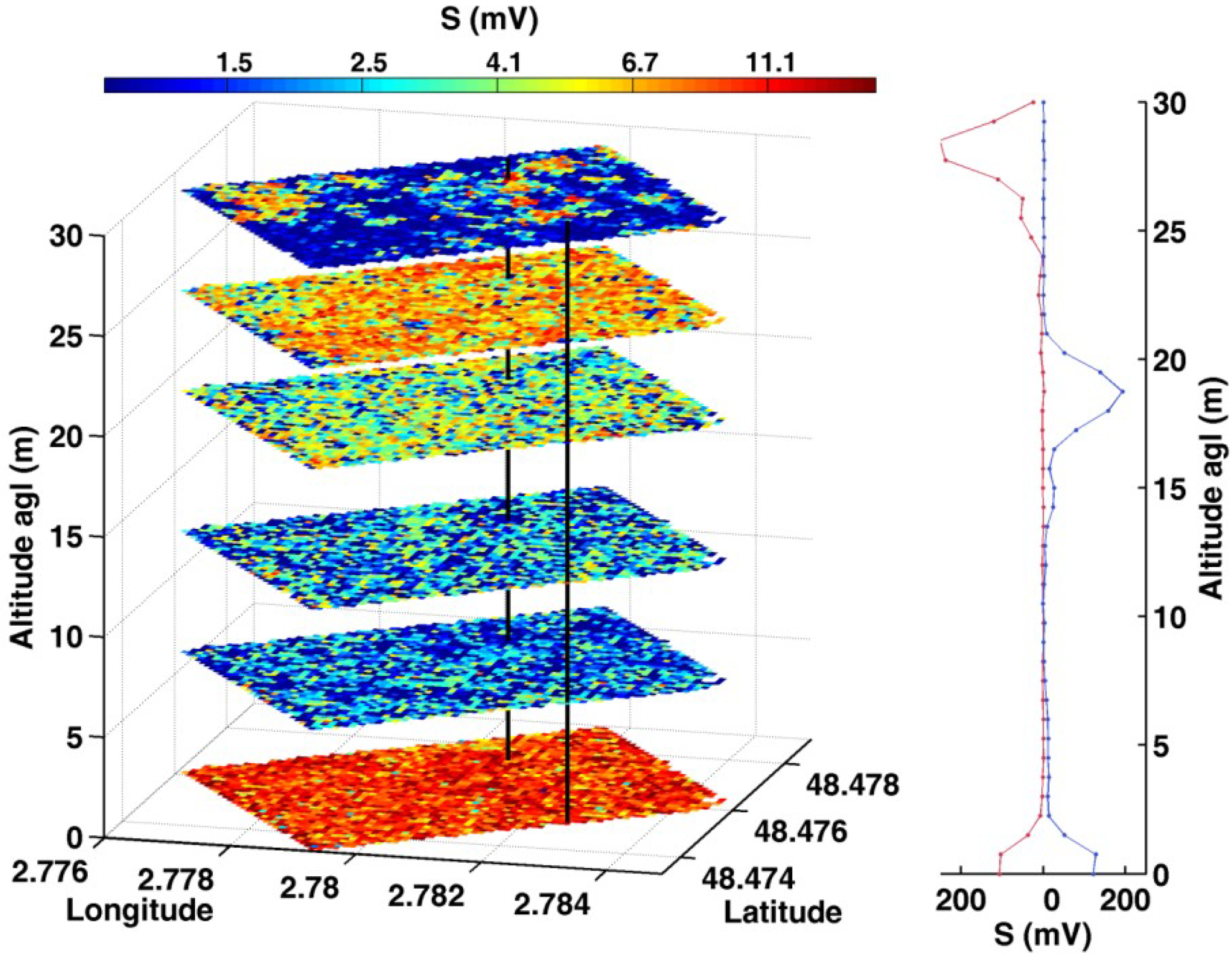
4.1. Forest Vertical Structures and Related Uncertainties
4.1.1. Thresholds Detection and Forest Vertical Structures

4.1.2. Uncertainties and Validation

| Uncertainty | Value | Uncertainty Elements | Estimate Sources |
|---|---|---|---|
| εTTH_lidar | 1.2 m | σTTH_lidar = 0.8 m, BTTH_lidar = 0.87 m | Lidar simulation (Monte Carlo) |
| εTTH_estimate | 2.6 m | σTTH_estimate(σTTH_field, σCBH_field) = 0.3 m, with σTTH_field = 1 m and σCBH_field = 0.02 m | Field measurements |
| σTTH_estimate(Regression) = 2.6 m | Regression fit | ||
| εAGCt_field | 9% | εAGCt_field(σTTH_estimate, σCBH_field) = 8% | Equation (11) |
| εAGCt_field(σα, σβ, σγ) = 4% | Allometric relationships Equation (11) | ||
| εAGC40_field | 4% | εAGC40_field(εAGCt_field) | Simulation (Monte Carlo) |
| εQMCH | 10% | σQMCH(SNR, Detection) = 10% | Lidar measurements |
| σQMCH(εGPS, εAHRS) = 0.12 m, with εGPS = 5 m and εAHRS = 3.6 m | Geolocation measurements | ||
| εAGC40_lidar | 16 tC ha‑1 | εAGC40_lidar(Regression)= 12 tC ha‑1 | Regression fit Equation (13), Figure 8 |
| εAGC40_lidar(εQMCH) = 11% | Equation (13) |
4.2. AGC Assessment and Related Uncertainties
4.2.1. Field-Derived AGC and Related Uncertainties
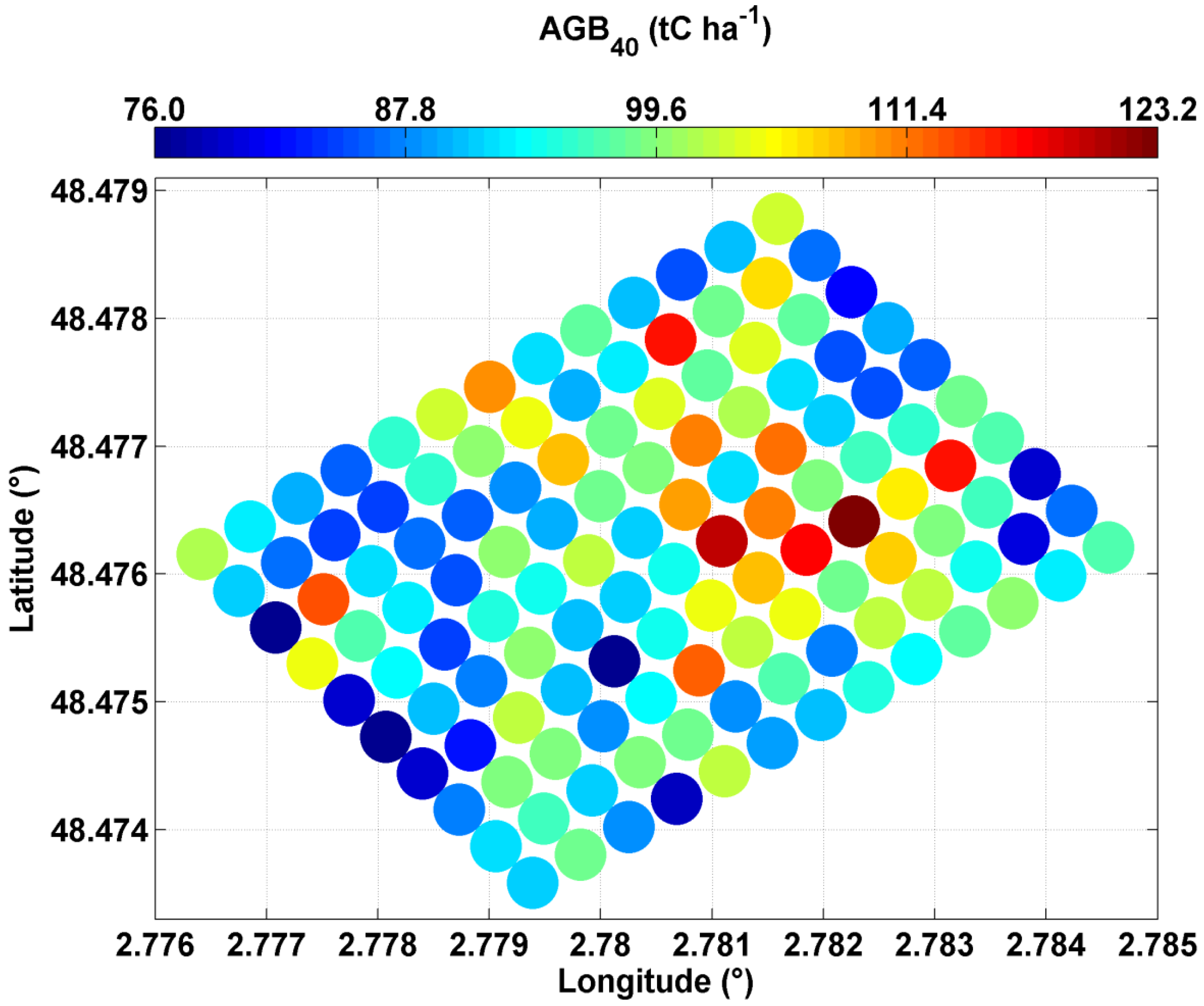
4.2.2. Lidar-Estimated AGC and Related Uncertainties
4.2.2.1. Uncertainties on the Lidar-Derived QMCH


4.2.2.2. Uncertainties on the Lidar-Derived AGC40
4.2.2.3. Discussion of the AGC40 and Its Uncertainty
| Location | Forest type | AGC (tC ha−1) | σAGC (tC ha−1) | Data type | References |
|---|---|---|---|---|---|
| Fontainebleau forest, France | Deciduous trees (oak, hornbeam) | 96 | 16 | LMe | This work |
| Fontainebleau forest, France | Deciduous trees (oak) | 110 | - | Mo | Le Maire et al. [29] |
| Total (oak, fagus, pinus) | 88.5 | ||||
| Central France | Sessil oak | 106 | - | Mo | Vallet et al. [40] |
| LopéNational Park, centre Gabon | Tropical rainforest | 172.6 | 48.8 | LMe | Mitchard et al. [41] |
| North America | Deciduous forest (oaks, hickories, beechs, tulip-populars) | 118 | 37.6 | LMe | Lefsky et al. [31] |
| Western cascades of Oregon, Pacific Northwest | Young conifer forests | 106.5 | 33.5 | FMe | Means et al. [17] |
| Mature conifer forests | 246 | 86 | |||
| North Island, New Zealand | Radiata pine dominated forests | 117 | 23 | LMe | Stephens et al. [42] |
| Southeastern Norway, Norway | Boreal forest | 50.6 | 0.8 | LMe | Næsset et al. [43] |
| Spruce, Scots pine | 58 | 1.85 | FMe |
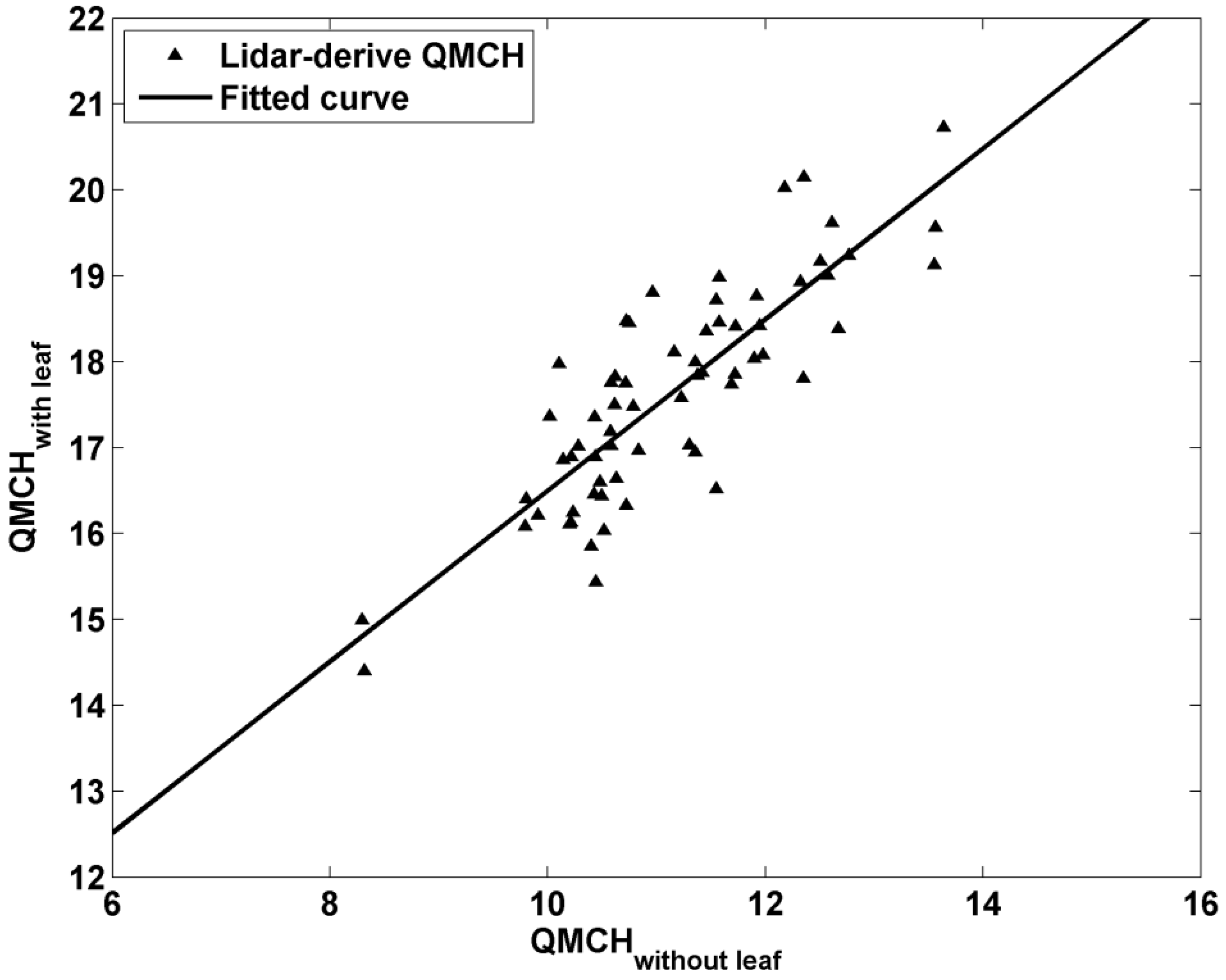
4.3. Leaf Effect

5. Conclusions
Acknowledgments
Author Contributions
Conflicts of Interest
References
- Anonymous. Climate Change 2013: The Physical Science Basis. Intergovernmental Panel on Climate Change (IPCC): Geneva, Switzerland, 2013; Chapter 6; pp. 465–570. [Google Scholar]
- Gibbs, H.K.; Brown, S.; Niles, J.O.; Foley, J.A. Monitoring and estimating tropical forest carbon stocks: Making REDD a reality. Environ. Res. Lett. 2007, 2, 045023. [Google Scholar] [CrossRef]
- MacArthur, R.H.; MacArthur, J.W. On Bird Species Diversity. Ecology 1961, 42, 594–598. [Google Scholar] [CrossRef]
- Lefsky, M.A.; Cohen, W.B. Lidar remote sensing of above- ground biomass in three biomes. Glob. Ecol. Biogeogr. 2002, 11, 393–399. [Google Scholar] [CrossRef]
- Brown, S.; Pearson, T.; Slaymaker, D.; Ambagis, S.; Moore, N.; Novelo, D.; Sabido, W. Creating a virtual tropical forest from three-dimensional aerial imagery to estimate carbon stocks. Ecol. Appl. 2005, 15, 1083–1095. [Google Scholar] [CrossRef]
- Cuesta, J.; Chazette, P.; Allouis, T.; Flamant, P.H.; Durrieu, S.; Sanak, J.; Genau, P.; Guyon, D.; Loustau, D.; Flamant, C. Observing the Forest Canopy with a New Ultra-Violet Compact Airborne Lidar. Sensors 2010, 10, 7386–7403. [Google Scholar] [CrossRef]
- Allouis, T.; Durrieu, S.; Chazette, P.; Bailly, J.S.; Cuesta, J.; Véga, C.; Flamant, P.; Couteron, P. Potential of an ultraviolet, medium-footprint lidar prototype for retrieving forest structure. ISPRS J. Photogramm. Remote Sens. 2011, 66, S92–S102. [Google Scholar] [CrossRef]
- Garvin, J.; Bufton, J.; Blair, J.; Harding, D.; Luthcke, S.; Frawley, J.; Rowlands, D. Observations of the earth’s topography from the Shuttle Laser Altimeter (SLA): Laser-pulse echo-recovery measurements of terrestrial surfaces. Phys. Chem. Earth 1998, 23, 1053–1068. [Google Scholar] [CrossRef]
- Harding, D.J.; Lefsky, M.A.; Parker, G.G.; Blair, J.B. Laser altimeter canopy height profiles methods and validation for closed-canopy, broadleaf forests. Remote Sens. Environ. 2001, 76, 283–297. [Google Scholar] [CrossRef]
- Brenner, A.C.; Zwally, H.J.; Bentley, C.R.; Csathó, B.M.; Harding, D.J.; Hofton, M.A.; Minster, J.-B.; Roberts, L.; Saba, J.L.; Thomas, R.H.; et al. Derivation of Range and Range Distributions From Laser Pulse Waveform Analysis for Surface Elevations, Roughness, Slope, and Vegetation Heights. In Geoscience Laser Altimeter System (GLAS) Algorithm Theoretical Basis Document; Version 4.1; Goddard Space Flight Center: Greenbelt, MD, USA, 2003; pp. 1–92. [Google Scholar]
- Schutz, B.E.; Zwally, H.J.; Shuman, C.A.; Hancock, D.; DiMarzio, J.P. Overview of the ICESat Mission. Geophys. Res. Lett. 2005, 32. [Google Scholar] [CrossRef]
- Harding, D.J. ICESat waveform measurements of within-footprint topographic relief and vegetation vertical structure. Geophys. Res. Lett. 2005, 32. [Google Scholar] [CrossRef]
- Lefsky, M.A.; Harding, D.J.; Keller, M.; Cohen, W.B.; Carabajal, C.C.; Del Bom Espirito-Santo, F.; Hunter, M.O.; de Oliveira, R. Estimates of forest canopy height and aboveground biomass using ICESat. Geophys. Res. Lett. 2005, 32, L22S02. [Google Scholar] [CrossRef]
- Zolkos, S.G.; Goetz, S.J.; Dubayah, R. A meta-analysis of terrestrial aboveground biomass estimation using lidar remote sensing. Remote Sens. Environ. 2013, 128, 289–298. [Google Scholar] [CrossRef]
- Wulder, M.A.; White, J.C.; Bater, C.W.; Coops, N.C.; Hopkinson, C.; Chen, G. Lidar plots—A new large-area data collection option: Context, concepts, and case study. Can. J. Remote Sens. 2012, 38, 600–618. [Google Scholar] [CrossRef]
- Le Toan, T.; Quegan, S.; Davidson, M.W.J.; Balzter, H.; Paillou, P.; Papathanassiou, K.; Plummer, S.; Rocca, F.; Saatchi, S.; Shugart, H.; et al. The BIOMASS mission: Mapping global forest biomass to better understand the terrestrial carbon cycle. Remote Sens. Environ. 2011, 115, 2850–2860. [Google Scholar] [CrossRef]
- Means, J.E.; Acker, S.A.; Harding, D.J.; Blair, J.B.; Lefsky, M.A.; Cohen, W.B.; Harmon, M.E.; McKee, W.A. Use of large-footprint scanning airborne Lidar to estimate forest stand characteristics in the western cascades of Oregon. Remote Sens. Environ. 1999, 67, 298–308. [Google Scholar] [CrossRef]
- Grant, R.H.; Heisler, G.M.; Gao, W.; Jenks, M. Ultraviolet leaf reflectance of common urban trees and the prediction of reflectance from leaf surface characteristics. Agric. For. Meteorol. 2003, 120, 127–139. [Google Scholar] [CrossRef]
- Ceccaldi, M.; Delanoë, J.; Hogan, R.J.; Pounder, N.L.; Protat, A.; Pelon, J. From CloudSat-CALIPSO to EarthCare: Evolution of the DARDAR cloud classification and its comparison to airborne radar-lidar observations. J. Geophys. Res. Atmos. 2013, 118, 7962–7981. [Google Scholar] [CrossRef]
- Sugimoto, N.; Nishizawa, T.; Shimizu, A.; Okamoto, H. AEROSOL classification retrieval algorithms for EarthCARE/ATLID, CALIPSO/CALIOP, and ground-based lidars. In Proceedings of the 2011 IEEE International Geoscience and Remote Sensing Symposium (IGARSS), Vancouver, BC, USA, 24–29 July 2011; pp. 4111–4114.
- Ansmann, A.; Wandinger, U.; Le Rille, O.; Lajas, D.; Straume, A.G. Particle backscatter and extinction profiling with the spaceborne high-spectral-resolution Doppler lidar ALADIN: Methodology and simulations. Appl. Opt. 2007, 46, 6606–6622. [Google Scholar] [CrossRef]
- Andersson, E.; Dabas, A.; Endemann, M.; Ingmann, P.; Källén, E.; Offiler, D.; Stoffelen, A. ADM-AEOLUS: Science Report; Clissold, P., Ed.; ESA Communication Production Office: Noordwijk, The Netherlands, 2008. [Google Scholar]
- Air Création. Available online: http://www.aircreation.fr (accessed on 13 June 2014).
- Chazette, P.; Sanak, J.; Dulac, F. New approach for aerosol profiling with a lidar onboard an ultralight aircraft: Application to the African Monsoon Multidisciplinary Analysis. Environ. Sci. Technol. 2007, 41, 8335–8341. [Google Scholar] [CrossRef]
- Quantel. Available online: http://www.quantel-laser.com/ (accessed on 13 June 2014).
- National Instruments. Available online: http://france.ni.com/ (accessed on 13 June 2014).
- Xsens. Available online: http://www.xsens.com/ (accessed on 13 June 2014).
- ONF. Available online: http://www.onf.fr/ (accessed on 13 June 2014).
- Le Maire, G.; Davi, H.; Soudani, K.; François, C.; Le Dantec, V.; Dufrêne, E. Modeling annual production and carbon fluxes of a large managed temperate forest using forest inventories, satellite data and field measurements. Tree Physiol. 2005, 25, 859–872. [Google Scholar] [CrossRef]
- Corif. Available online: http://www.corif.net/site/sitesobs/ (accessed on 13 June 2014).
- Lefsky, M.A.; Harding, D.; Cohen, W.B.; Parker, G.; Shugart, H.H. Surface lidar remote sensing of basal area and biomass in deciduous forests of eastern Maryland, USA. Remote Sens. Environ. 1999, 67, 83–98. [Google Scholar] [CrossRef]
- Chazette, P.; Pelon, J.; Mégie, G. Determination by spaceborne backscatter lidar of the structural parameters of atmospheric scattering layers. Appl. Opt. 2001, 40, 3428–3440. [Google Scholar] [CrossRef]
- Measures, R.M. Laser Remote Sensing: Fundamentals and Applications; Wiley, J., Ed.; Krieger Publishing Company: Malabar, FL, USA, 1984; p. 510. [Google Scholar]
- MacArthur, R.H.; Horn, H.S. Foliage Profile by Vertical Measurements. Ecology 1969, 50, 802–804. [Google Scholar] [CrossRef]
- Brown, S. Measuring carbon in forests: Current status and future challenges. Environ. Pollut. 2002, 116, 363–372. [Google Scholar] [CrossRef]
- De Dhôte, J.-F.; De Hercé, É. Un modèle hyperbolique pour l’ajustement de faisceaux de courbes hauteur–diamètre. Can. J. For. Res. 1994, 24, 1782–1790. [Google Scholar] [CrossRef]
- Vallet, P.; Dhôte, J.F.; Moguédec, G.L.; Ravart, M.; Pignard, G. Development of total aboveground volume equations for seven important forest tree species in France. For. Ecol. Manag. 2006, 229, 98–110. [Google Scholar] [CrossRef]
- Boudreau, J.; Nelson, R.F.; Margolis, H.A.; Beaudoin, A.; Guindon, L.; Kimes, D.S. Regional aboveground forest biomass using airborne and spaceborne LiDAR in Québec. Remote Sens. Environ. 2008, 112, 3876–3890. [Google Scholar] [CrossRef]
- Casella, G.; Berger, R.L. Statistical Inference, 2nd ed.; Duxbury Press: Pacific Grove, CA, USA, 2001; pp. 240–245. [Google Scholar]
- Vallet, P.; Meredieu, C.; Seynave, I.; Bélouard, T.; Dhôte, J.F. Species substitution for carbon storage: Sessile oak versus Corsican pine in France as a case study. For. Ecol. Manag. 2009, 257, 1314–1323. [Google Scholar] [CrossRef]
- Mitchard, E.T.A.; Saatchi, S.S.; White, L.J.T.; Abernethy, K.A.; Jeffery, K.J.; Lewis, S.L.; Collins, M.; Lefsky, M.A.; Leal, M.E.; Woodhouse, I.H.; et al. Mapping tropical forest biomass with radar and spaceborne LiDAR in Lopé National Park, Gabon: Overcoming problems of high biomass and persistent cloud. Biogeosciences 2012, 9, 179–191. [Google Scholar]
- Stephens, P.R.; Watt, P.J.; Loubster, D.; Haywood, A.; Kimberley, M.O. Estimation of carbon stocks in New Zealand planted forests using airborne scanning LiDAR. In Proceedings of the ISPRS Workshop on Laser Scanning 2007 and SilviLaser 2007, Espoo, Finland, 12–14 September 2007.
- Næsset, E.; Gobakken, T.; Solberg, S.; Gregoire, T.G.; Nelson, R.; Ståhl, G.; Weydahl, D. Model-assisted regional forest biomass estimation using LiDAR and InSAR as auxiliary data: A case study from a boreal forest area. Remote Sens. Environ. 2011, 115, 3599–3614. [Google Scholar] [CrossRef]
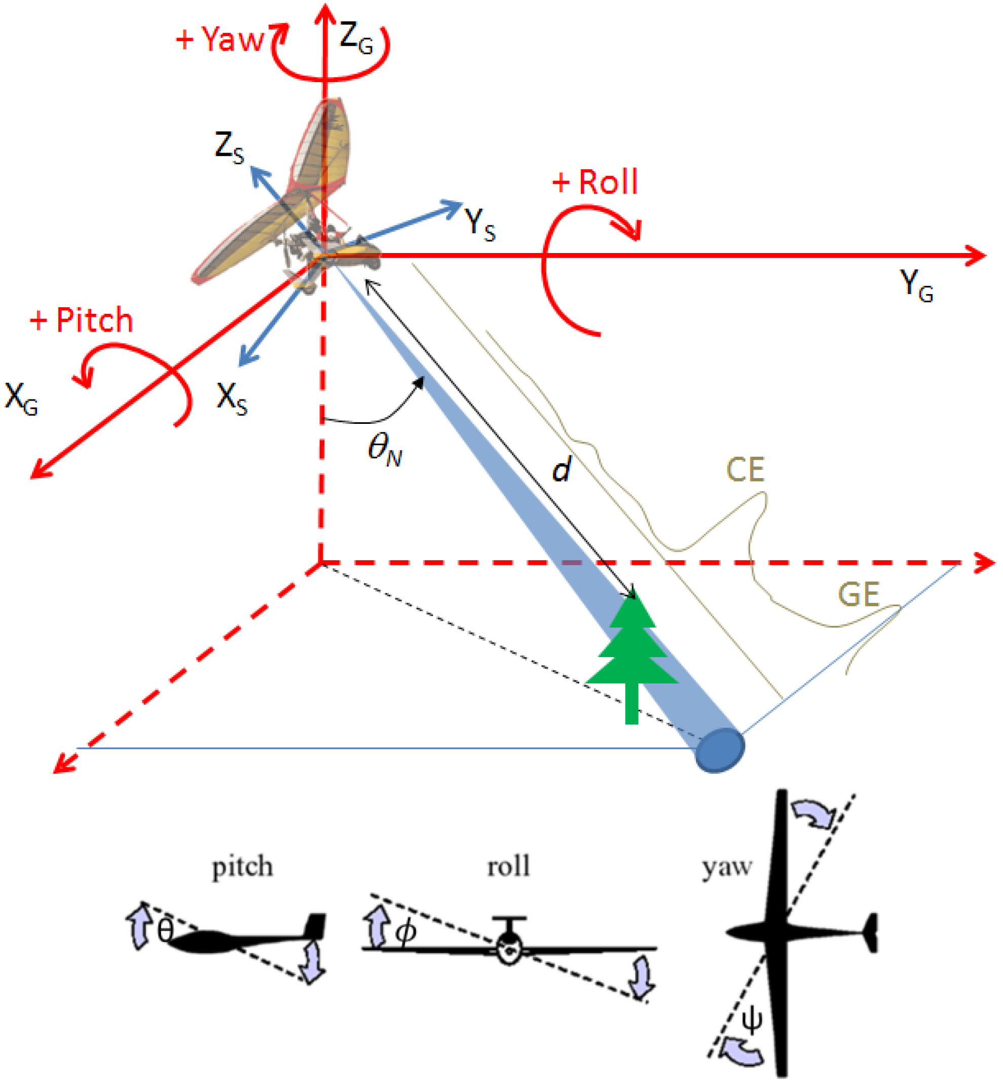
Appendix A: Lidar Ground-Track Location (Geolocation)


© 2014 by the authors; licensee MDPI, Basel, Switzerland. This article is an open access article distributed under the terms and conditions of the Creative Commons Attribution license (http://creativecommons.org/licenses/by/3.0/).
Share and Cite
Shang, X.; Chazette, P. Interest of a Full-Waveform Flown UV Lidar to Derive Forest Vertical Structures and Aboveground Carbon. Forests 2014, 5, 1454-1480. https://doi.org/10.3390/f5061454
Shang X, Chazette P. Interest of a Full-Waveform Flown UV Lidar to Derive Forest Vertical Structures and Aboveground Carbon. Forests. 2014; 5(6):1454-1480. https://doi.org/10.3390/f5061454
Chicago/Turabian StyleShang, Xiaoxia, and Patrick Chazette. 2014. "Interest of a Full-Waveform Flown UV Lidar to Derive Forest Vertical Structures and Aboveground Carbon" Forests 5, no. 6: 1454-1480. https://doi.org/10.3390/f5061454
APA StyleShang, X., & Chazette, P. (2014). Interest of a Full-Waveform Flown UV Lidar to Derive Forest Vertical Structures and Aboveground Carbon. Forests, 5(6), 1454-1480. https://doi.org/10.3390/f5061454