Abstract
In this study, an Improved Zebra Optimization Algorithm (ZOA) is proposed based on the search mechanism of the Sparrow Optimization Algorithm (SSA), the perturbation mechanism of the Particle Swarm Algorithm (PSO), and the adaptive function. Then, Improved Zebra Optimization Algorithm (IZOA) was used to optimize the Deep Hybrid Kernel Extreme Learning Machine Model (DHKELM), and the IZOA-DHKELM was obtained. The model has been used to predict the color of heat-treated wood for different species, temperatures, times, media, and profile types. In this article, the original DHKELM and the ZOA-DHKELM were compared to verify the validity and accuracy of the model. The results indicated that the IZOA-DHKELM decreased the mean absolute error (MAE), root mean square error (RMSE), and mean absolute percentage error (MAPE) by 56.2%, 67.4%, and 34.2%, respectively, while enhancing the coefficient of determination, , to 0.9952 compared to the ZOA-DHKELM. This demonstrated that the model was significantly optimized, with improved generalization ability and prediction accuracy. It can better meet the actual engineering needs.
1. Introduction
Wood is a natural material widely used in construction and furniture production. However, the wood has many defects, such as poor dimensional stability, poor mechanical properties, and uneven wood color, which limit the range of applications. Wood modification can effectively address these natural defects of wood [1]. Wood heat treatment is the most common method of modifying wood. Heat-treated wood, as a special wood treated at high temperatures, has been widely used in outdoor and indoor furniture and other fields in recent years due to its unique carbonization process and excellent anti-corrosion and environmental protection properties [2]. In addition, the color change in heat-treated wood is an important feature of its treatment process, directly affecting the wood’s esthetic degree and practicality. Therefore, the accurate prediction of color changes in heat-treated wood is important for improving production efficiency and product quality.
Heat treatment causes the wood to darken, mostly to a dark brown. This is because heat treatment changes the main chemical composition of the wood. Cellulose, hemicellulose, and lignin are degraded to varying degrees, which leads to an increase in the concentration of phenolics and redox reactions that darken the color of the wood [3]. Heat-treated timber boasts a uniform color both inside and out, enhancing its overall esthetic appeal. In addition, heat-treated wood has better color stability under ultraviolet light than non-heat-treated wood [4]. Scholars have conducted many studies on the color change in heat-treated timber through experiments. A study by Sikora et al. [5] explores how varying heat treatment temperatures impact the color changes in spruce and oak wood. They found that the temperature gradually increased during heat treatment. The surface Lightness (L*) of the wood gradually decreased, and the maximum color difference (∆E) gradually increased. And the total color difference reached the maximum value at 210°. Aydemir et al. [6] investigated the effects of heat treatment on the color change in cypress, tertiary hazel, pendant, beech, cherry, and juniper, which were shown to be significant. Jiang et al. [7] experimentally concluded that heat treatment temperature and time are important factors affecting the color of rubberwood and that the color of rubberwood deepened gradually with the increase in heat treatment temperature and time. Jin et al. [8] conducted a study on how heat treatment affects the color change in various tree species, including pinus pinaster, larch, spruce, and boxwood. The experimental findings highlighted that each tree species exhibited a distinct degree of color transformation following the heat-treatment process. Liu et al. [9] heat-treated samples of eight different color tree species at different temperatures and times. The results showed that the brightness index of wood color parameters was more sensitive to the treatment conditions and decreased with increasing temperature and time, and this trend was the same for all wood samples, but the magnitude of the differences was greater among different wood species. Chen et al. [10] investigated the effects of oxygen content and moisture content on chemical and color changes during the heat treatment of acacia wood. The results show that decreases significantly with heat treatment, and increase gradually, and the total color difference () becomes larger and larger. The studies mentioned above indicate that the process is time-consuming and mention the material and financial resources required to study the color change in heat-treated wood by experimental means. Therefore, the color change in wood during the heat-treatment process can be predicted by mathematical modeling. The industry’s color requirements for heat-treated wood can be met more quickly and efficiently in practical applications [11].
At present, some scholars have studied the color change in heat-treated wood using models. Nguyen et al. [12] predicted the color change in wood in the heat-treatment process by using an artificial neural network model and obtained good prediction results, Li et al. [13] effectively used a support vector machine model to predict the color change in wood during artificial weathering following heat treatment, and Mo et al. [14] successfully predicted the color change in ash wood, yellow wood, and yellow wood in the process of heat treatment with the help of an artificial neural network. They successfully predicted the color changes in ash, boxwood, and red oak during heat treatment. ZOA is characterized by a strong optimization ability and a fast convergence speed although it is a relatively new metaheuristic algorithm. The DHKELM has been widely used for prediction in the past year, and it has been successfully applied in various fields, such as carbon emission and photovoltaic predictions [15,16]. Despite advancements in predictive modeling, the use of ZOA and DHKELMs to forecast the color of heat-treated wood has not yet been explored. Additionally, both ZOA and DHKELMs have certain limitations, and improving and combining these two can continue to optimize and improve how they work together.
This paper proposes an Improved Zebra Optimization Algorithm (IZOA) based on the sparrow search mechanism, particle swarm perturbation mechanism, and adaptive function, which is mainly aimed at the shortcomings of ZOA that it has a high probability of falling into a local optimum, has low flexibility for the speed of searching for the optimum, and is unable to verify its optimal solution. Then, the DHKELM was improved using IZOA, and the IZOA-DHKELM was proposed. This study aimed to effectively predict the color changes in heat-treated wood using the advanced IZOA-DHKELM. Additionally, it sought to showcase the model’s reliability in forecasting the physical properties of heat-treated wood. In addition, it provided some reference for the construction and furniture decoration industries.
2. IZOA-DHKELM Prediction Model
2.1. Basic Mechanisms of Deep Hybrid Kernel Extreme Learning Machine Models
The DHKELM [17] is an Extreme Learning Machine (ELM) model that combines deep learning with kernel methods. In this approach, deep layers are used instead of traditional basis function mappings to increase the complexity and learning ability of the model while still maintaining the efficiency and stability of ELM. Specifically, the DHKELM constructs complex nonlinear mappings through multiple hidden layers, usually parameterized using kernel functions. The DHKELM is improved by the continuous optimization of the ELM model.
(1) Hybrid Kernel Extreme Learning Machine
ELM is a machine learning algorithm for single-hidden layer feedforward neural networks (SLFNs). The network structure of ELM is the same as that of SLFN [18]. Still, traditional feedforward neural networks have obvious drawbacks, such as a slow training speed, easy falling into the local minima, and sensitive selection of the learning rate. The ELM algorithm compensates for these shortcomings by moving away from the tried-and-tested traditional neural network in the training stage to a gradient-based algorithm (backward propagation) but chooses to randomly generate the connection weights of the input layer and the hidden layer and the threshold of the hidden layer neurons. There is no need to adjust in the training process; you only have to set the number of hidden layer neurons, and you can obtain the unique optimal solution. Compared with the previous traditional training methods, the ELM method has the advantages of a fast learning speed and a good generalization ability.
It is assumed that there are N random sample data , where is the input, is the output, and = 1, 2, 3, …, n. The learning process of ELM is characterized by solving for the least squares solution, as shown in Equation (1).
where is the Moore–Penrose generalized inverse transform of matrix , is the target output matrix, and is the output weight matrix.
The ELM has limitations when dealing with more complex datasets, manifested in decreased stability and generalization ability. In contrast, the kernel function’s nonlinear mapping ability is very powerful, so the kernel function is introduced based on the ELM. The specific operation is to replace the random matrix with the kernel matrix, map the low-dimensional input samples to the high-dimensional kernel space, and determine the output weight matrix through the training samples and the kernel function. The Kernel Extreme Learning Machine (KELM) [19], constructed by combining kernel function and ELM, has stronger learning and generalization abilities. In this paper, the kernel function matrix is introduced, and its expression is as follows:
where is the kernel function, and is the kernel matrix.
Therefore, the model output expression of KELM is as follows:
where is the regularization factor, and is the unit matrix.
The kernel function is an important factor affecting KELM’s performance. A single kernel function makes it difficult to adequately learn data with nonlinear characteristics. To further improve KELM’s performance, the Radial Basis Function (RBF) and the Polynomial Kernel (Poly) have been chosen and combined with weighted parameters to create a hybrid kernel function [20].
The RBF can map the input samples to a high-dimensional space with better learning ability, and its kernel function expression is as follows:
where is the parameter of the RBF kernel function.
Poly has good generalization ability, and its kernel function expression is as follows:
where is a constant, and is the number of polynomials.
The expression of the hybrid kernel function after RBF and poly-weighted summation is as follows:
where is the hybrid kernel function weight coefficient.
(2) Deep Hybrid Kernel Extreme Learning Machine
Autoencoder (AE) [21] is a handy unsupervised learning algorithm in deep learning. Its basic idea is the mapping of input data to a low-dimensional potential space and then the reconstruction of the original data from this potential space, i.e., data dimensionality reduction, feature extraction, and data reconstruction. AE has a strong advantage in terms of learning ability and generalization abilities. The ELM is combined with AE. The Extreme Learning Machine Auto-Encoder (ELM-AE) is a variant of the ELM, which can efficiently learn important features from the input data and maintain the symmetry between input and output. The Deep Extreme Learning Machine (DELM) constitutes the ELM-AE as a basic cascade unit, which first performs unsupervised deep feature extraction using the ELM-AE and then supervised classification via the ELM.
The DHKELM combines the features of the DELM and HKELM, and its structure is schematically shown in Figure 1 Its initialization process is shown as follows:
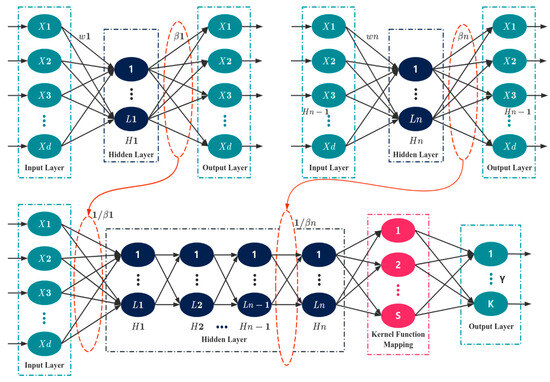
Figure 1.
DHKELM structural diagram.
Step 1: the randomly initialized input weights and bias in the ELM-AE model are orthogonalized.
Step 2: the output matrix and output weights corresponding to the nodes of the implicit layer can be derived by Equations (7) and (8).
where is the activation function, and is the input sample.
Step 3: the implied layer output matrix of the ELM-AE for each layer is calculated by Equation (9).
The output of the DHKELM is as follows:
2.2. The Traditional Zebra Optimization Algorithm
In 2022, Trojovská et al. introduced an innovative approach to solve complex optimization problems: the ZOA metaheuristic algorithm [22]. This concept draws inspiration from the natural behavior of wild zebras. ZOA simulates zebras’ foraging behavior and defense strategies against predator attacks. Considering that ZOA is characterized by strong optimization-seeking capability and high speed of convergence, the algorithm is selected for improvement. Its mathematical modeling process is as follows.
(1) Initialization
Similar to other optimization algorithms, ZOA starts by randomly initializing the population in the optimization space:
where is an individual, is the lower boundary of the search for superiority, is the upper boundary of the search for superiority, and is a random number between [0, 1].
(2) Phase I: Foraging Behavior
In the first phase, population members were updated based on the simulations of zebra behavior when searching for forage. Among zebras, there is a type of zebra called plains zebra, which is a pioneer herbivore. Plains zebras actively choose harder-to-obtain and less nutritious foods when feeding and give up easier-to-obtain and more nutritious foods to other zebras. In ZOA, the best member of the population is considered to be the pioneer zebra, which is responsible for leading the other members of the population towards its position in the search space. Therefore, updating the zebra’s position in the foraging phase can be mathematically modeled using Equation (12) and Equation (13).
where is the pioneer zebra, is a random number between the interval [0, 1], and I is a random value in the set .
(3) Phase II: Defense Strategies Against Predators
In the second phase, zebra defense strategies against predator attacks were simulated to update the position of ZOA population members in the search space. Zebras’ main predators are lions; however, they are also threatened by cheetahs, leopards, wild dogs, and other animals. Crocodiles can also be the potential predators of zebras when they approach water. The zebra’s defense strategy changes depending on the predator. When faced with a lion attack, the zebra choose an escape strategy characterized by fleeing in zigzag routes and random lateral turning movements. When faced with a small predator, such as a wild dog, zebras choose a defense strategy, manifested by other zebras in the population approaching the attacked zebra and working together to build a defense structure against the predator. In the ZOA design, it is assumed that the above two situations occur with equal probability. In this paper, we mathematically model the two defense strategies of zebras, as shown in Equation (14).
where denotes the zebra’s escape strategy against lions, denotes the fending-off strategy against cheetahs and wild dogs, is the number of iterations, is the maximum number of iterations, is a constant of 0.01, is the switching probability of the two strategies with a random value between [0, 1], and is the state of the attacked zebra.
When updating the zebra’s position, if the zebra has a better target value in the new position, it accepts the new position. If the zebra’s target value in the new position is not as good as the target value in the original position, the zebra still maintains the original position. This update condition can be modeled by Equation (15).
2.3. The Improved Zebra Optimization Algorithm
2.3.1. Introduction of a Sparrow Search Mechanism
In the traditional ZOA, the foraging behavior of the zebra herd is drawn from the pioneer zebra, and this exploitation pattern accelerates the convergence of ZOA during the mid and late stages. However, when pioneer zebras are poorly positioned or trapped in local optimalit, the refined search around ZOA will result in the population moving toward early maturity. To address this problem, this paper chooses to refine the search mechanism. Sparrow Optimization Algorithm (SSA) [23] has been proven to have a strong global exploration ability and is widely used in various optimization scenarios. In this paper, based on ZOA, the foraging process of sparrow searchers in SSA is introduced to supplement ZOA, and the proportion of explorers is set to be 70%. The leader position update rule for the SSA can be found in Equation (16):
where is the current best position, is the individual’s current position, and is a random number in the range of [0, 1].
In addition, the safety of the foraging process can be ensured by utilizing the early warning mechanism of SSA, avoiding natural enemies. The position update rule of SSA avoiding natural enemies is shown in Equation (17):
where is the worst position in the population, representing the position where the natural enemy may appear, and is a random number in the range of [0, 1].
The introduction of the sparrow foraging mechanism enriches the search strategy of ZOA, and its S-exponential step is conducive to expanding the search range of the current solution. This solves the problem that ZOA can easily fall into the local optimum.
2.3.2. Introducing an Adaptive Exponential Function Instead of the Escape Factor
The search speed of ZOA greatly affects its search quality. In the traditional ZOA, its speed is mainly affected by the evasion factor . And is a constant of 0.01, which leads to the search speed not being adjusted with the search process. It is considered that ZOA has different requirements for the search speed at different search stages. In the early search stage, searching as many solutions as possible in the largest possible search range at a fast speed is necessary. When entering the middle and late stages of the search, the search quality needs to be improved by reducing the search speed to avoid omitting the better solutions. Therefore, in this paper, the evasion factor is adjusted from a constant to a nonlinearly decreasing exponential function, as shown in Equation (18):
As shown in Figure 2, the escape factor decreases gradually from 0.6 to converge to 0.1 as increases.
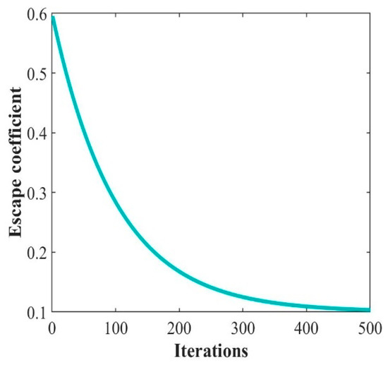
Figure 2.
Trend of decreasing escape factor .
2.3.3. Introduction of Particle Swarm Perturbation Mechanism
In the search optimization process, ZOA consistently explores the search space to identify improved solutions based on the existing ones. However, whether the current solution is optimal at the moment and whether the new solution searched afterward is better than the current optimal solution cannot be verified. The particle swarm perturbation mechanism can achieve the verification of the ZOA solution through the reverse search and has been applied many times in previous algorithm improvements. Therefore, the speed update rule of the Particle Swarm Algorithm is introduced to verify the optimal solution instantly, as shown in Equation (19) [24]:
where is the inertia weight, are random numbers in the interval [0, 1], is the velocity vector of particle in the dth dimension in the kth iteration, is the individual learning factor, is the population learning factor, is the historical optimal position of particle in the dth dimension in the kth iteration, is the particle in the kth iteration position vector in the dth dimension, and is the historical optimal position of population in the dth dimension in the kth iteration.
In summary, the Improved Zebra Optimization Algorithm (IZOA) is quoted by combining the search mechanism of SSA, the adaptive exponential function, and the perturbation mechanism of PSO in the improvement of the traditional ZOA in terms of three perspectives of globalization, search speed, and optimal solution verification.
2.4. The IZOA-DHKELM
This research introduces an enhanced Zebra Optimization Algorithm aimed at optimizing a Deep Hybrid Kernel Extreme Learning Machine Model, developed using MATLAB (2020b). The process is as follows. Firstly, the inputs and outputs of the model are determined. To effectively organize your sample data, it should be divided into two distinct categories: a training set and a testing set. Then, 70% of the data for training purposes and 30% for testing should be allocated. The entire dataset should be normalized to ensure consistent and meaningful results. Next, the parameters are set, the number of hidden layers of the model is set to three layers, the type of ELM-AE activation function is sigmoid, the two types of kernel function of the top hybrid kernel limit learning machine are RBF kernel function and Poly kernel function, and the parameter optimization range is determined according to the type of kernel function. Then, the population parameters are optimized using the Improved Zebra Optimization Algorithm, setting the number of populations to 30 and the maximum number of iterations to 50, calculating the fitness values of the populations, and updating their speed, position, and other parameters to determine the end conditions of the optimal parameters. The IZOA-DHKELM’s prediction performance is thoroughly evaluated using the test dataset. If the predicted values meet the set requirements, they will be the output. If not, the parameters will continue to be optimized until the end conditions are met. The process is shown in Figure 3.
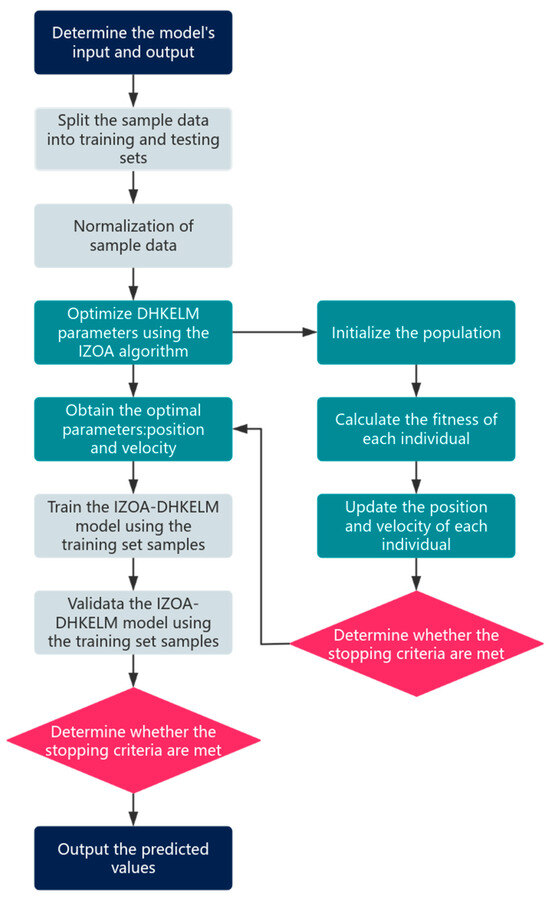
Figure 3.
IZOA-DHKELM flowchart.
3. Experimental
3.1. Data Collection and Pre-Processing
The literature [25] provided test data for this paper. The literature tested pinus pinaster and eucalyptus wood for changes in wood color under different heat treatment conditions. The color data before heat treatment are shown in Appendix A, Table A1, and the dataset after heat treatment is shown in Appendix A, Table A2.
The experimental procedure in the literature [25] is as follows. Test samples of pinus pinaster and eucalyptus cubes with edges of about 40 mm were cut from radial boards with smooth surfaces, with a total of 150 samples of each species. The samples were sandpapered and kept in a conditioned room at a temperature of 20 °C and 50% relative humidity until stabilized. Before heat treatment, the color of the samples was measured radially, tangentially, and cross-sectionally. The specimens were then heat-treated as follows: (1) in an oven with air and (2) in an autoclave without air for steam heat treatment. The air heat treatment was carried out in an electric oven with natural convection exhaust of hot air through the ko ports in the oven wall, at temperatures ranging from 170 to 200 °C, for a treatment time of 2–24 h. Treatments were started at ambient temperature with a ramp-up time of approximately 1 h. Four replications were performed for each treatment time/temperature condition. Steam heat treatment was performed in an autoclave at 190–210 °C for 2–12 h. The autoclave had a capacity of 0.5 m3 and an area of 1.0 m2 and was heated by regulating the entry of a mixture of superheated steam (370–380 °C) and saturated steam (150–160 °C). The temperature was controlled by assisted heating by a stream of superheated steam in the autoclave sleeve, with three replicates for each time/temperature treatment condition.
In predicting lumber color using the IZOA-DHKELM, we utilized the initial 70% of the data from Table A2 in Appendix A as the training set. The other 30% was used as the test set. Tree species, heat-treatment temperature, heat-treatment time, heat-treatment medium, and test timber profile type were the input parameters, and total color change (∆E) was used as an output parameter. Since the size of the data is different between the four input parameters of the model, the input data were standardized in this article using the min–max normalization method. Equation (20) performs a linear transformation on the original data to map the resultant values to the specified range [26].
is the normalized original data, is the normalized value, is the maximum value of the initial data, and is the minimum value. The process of data normalization involves scaling data so that the data consistently fit within the [0, 1] range. This method helps preserve the original data distribution pattern, ensuring accurate analysis and interpretation [27].
3.2. Color Measurement
The following measurements were made in the literature [25] for wood color. The final color of the wood is measured after stabilization in a room at 20 °C and 50% relative humidity radially, tangentially, and cross-sectionally. The Minolta cm-3630 Colorimetric Spectrophotometer is calibrated with the white standard for 0% color and the black standard for 100% color. The color parameters , , and were measured by the CIELAB method [28]. And their changes , and before and after heat treatment were calculated. The total color change (∆E) has been computed according to the formula as follows:
where , , and represents the changes in color coordinates. , , and denote the luminance, red-green coordinate, and yellow-blue coordinate of the untreated specimen, and , , and denote the luminance, red-green coordinate and yellow-blue coordinate of the treated specimen.
3.3. Model Parameter Setting
3.3.1. Metaheuristic Algorithm Parameterization
To assess the effectiveness of IZOA, we conducted a performance comparison with traditional ZOAs and popular metaheuristics (MAs). The preferred algorithm features are as follows: the Golden Jackal Optimization Algorithm (GJO) [29], the Nighthawk Optimization Algorithm (NGO) [30], the Gray Wolf Optimization Algorithm (GWO) [31], and the Honey Badger Optimization Algorithm (HBA) [32]. Table 1 provides the detailed parameter settings for each metaheuristic algorithm. In order to ensure equity, each metaheuristic algorithm was configured with a maximum of 500 iterations and a population size of 30.

Table 1.
Parameter settings of MHA.
3.3.2. IZOA-DHKELM Parameter Setting
In this study, the IZOA-DHKELM adopts a three-layer structure, including the input, implied, and output layers. The input layer consists of five nodes, each representing a different heat treatment temperature, heat treatment time, heat treatment tree species, heat treatment medium, and profile type. The output layer consists of a single node that represents the wood’s color. The model’s population is 30, the maximum number of iterations is 50, and the implicit layer is set to three layers. Determining the type of activation function for the model is also one of the most important steps in the construction of the model. The activation function is essential in a neural network model as it introduces nonlinearities. This ability allows the network to effectively learn and depict intricate patterns and relationships. If there is no activation function, the neural network can only represent linear transformations, greatly restricting the ability of neural networks to express themselves. Commonly used activation functions in the model are tansig, relu, sigmoid, purelin, and so on. This paper highlights the selection of the sigmoid activation function, a popular choice for neural networks. The sigmoid function is chosen for its ability to constrain output values between 0 and 1, making it an ideal tool for addressing nonlinear problems.
When developing a model, it is crucial to establish the optimization boundaries, determine the number of nodes for each layer within the implicit layer, and select the appropriate kernel function. These factors will significantly influence the optimization dimension. Thus, the optimization range should be set in segments. The first is to set the number of nodes in each layer; the number of nodes in the hidden layer determines the complexity and learning ability of the network, and the final setting range is an integer between 1 and 100. The second is the setting of regularization coefficients and weighting coefficients, adding the boundaries of ELM-AE regularization coefficients, HKELM penalty coefficients, and Kernel weighting coefficients, setting the minimum value of 0.001, the maximum value of 1000, and weighting coefficients in the range of 0 to 1. The tuning coefficients help prevent superficial overfitting and improve the model’s ability to generalize. Finally, in the kernel function settings, you need to set the optimization range of the kernel parameters according to the type of the selected kernel function, and you can dynamically adjust the parameter range according to the needs of different combinations. The model constructs a very systematic mechanism for setting the range of nuclear parameters, which is selected by combining various types of atomic functions, specifically RBF kernel and RBF kernel combination, RBF kernel and linear kernel combination, RBF kernel and poly kernel combination, RBF kernel and fluctuation kernel combination, linear kernel and linear kernel combination, linear kernel and poly kernel combination, linear kernel and fluctuation kernel combination, polynomial kernel and polynomial kernel combination, polynomial kernel and fluctuation kernel combination, and fluctuation kernel and fluctuation kernel combination, by assigning the parameters in this way, and it is ensured that the correct kernel parameters and control terms are used. After training on the dataset of this paper, the RBF kernel function and poly kernel function are selected; the RBF kernel can handle complex classification problems, and the poly kernel forces complex nonlinear problems.
3.4. Model Performance Evaluation
In this paper, mean square error (MSE), mean absolute error (MAE), root mean square error (RMSE), mean absolute percentage error (MAPE), and coefficient of determination () have been selected as key indicators for assessing the model’s accuracy and precision. The scores for each evaluation metric were calculated using the following Equation (25)–(29) [33].
where is the actual value of the experimental sample, is the predicted value, represents the volume of data, and is the average of all actual values.
4. Results and Discussion
4.1. Validation of the Effectiveness of the IZOA
To accurately evaluate IZOA compliance and determine the success of IZOA enhancement strategies, we conduct performance testing using the widely recognized 23 sets of test functions [34]. These evaluations ensure that IZOA delivers optimal results and meets industry standards. F1 to F7 are unimodal benchmark test functions, F8 to F13 are multimodal benchmark test functions, and F14 to F23 are composite benchmark test functions. Among them, F1 to F13 dimensions are 30, and F14 to F23 dimensions vary from 2 to 6. In this paper, 4 of the 23 groups of test functions are selected for demonstration. These include the spherical function F1, which is a simple and representative benchmark test function commonly used to test the performance of algorithms on simple convex optimization problems; the cumulative sum of squares function F3, which exists multiple local optimizations, increasing the difficulty of the optimization algorithm, and requires the process to obtain a good global searching due to the discontinuity of the gradient information; the maximum function F4 is a nonsmoothed function whose goal is to find the element of the input vector with the largest absolute value, and although the function itself is relatively simple, solving the maximum problem requires a global search strategy; and hybrid function F13, which has complex nonlinear interactions and requires the optimization algorithm to consider both global and local search strategies, which can effectively evaluate the ability of the algorithm. The detailed description of the selected test functions is shown in Table 2.
Table 2.
Specific information about the test function.
In the experiments, the IZOA has been in comparison with the unenhanced ZOA and several other algorithms with superior performance, including GJO, NGO, GWO, and HBA. The population size was set to 30, with a maximum of 500 iterations, and each algorithm underwent a single independent run. The results of the analysis are shown in Figure 4.
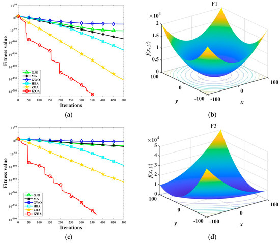
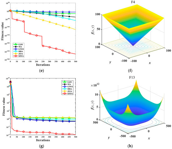
Figure 4.
Convergence curves of each algorithm on different test functions: (a) F1; (b) Fl; (c) F3; (d) F3; (e) F4; (f) F4; (g) F13; and (h) F13.
Figure 4 visualizes each algorithm’s convergence curves in different dimensions and test functions. During the testing process, it becomes evident that GJO, NGO, GWO, and HBA stop iterating before finding the optimal solution, indicating that these algorithms are easily affected by the local optimum. ZOA outperforms the previous algorithms but is also affected by the local optimum, decreasing the solution accuracy. IZOA has the fastest converging speed and highest converging accuracy, with an almost linear convergence process, showing a superior convergence speed. It shows a superior convergence speed for the GJO, NGO, GWO, HBA, and ZOAs. As the IZOA nears the optimal solution, significant enhancements become evident. The remaining algorithms continue to iterate towards the best solution, showcasing IZOA’s remarkable convergence rate.
Meanwhile, IZOA can be very close to the optimal solution for these test functions after reaching the final number of iterations. Simultaneously, after finishing the last set of iterations, the alternative algorithms continue to show a notable difference from the optimal solution. This example highlights the exceptional accuracy and stability of IZOA when tackling high-dimensional problems. It should be discovered how IZOA consistently delivers superior performance in complex scenarios.
4.2. Model Prediction Results
When evaluating algorithm performance, the enhanced IZOA demonstrates an exceptional convergence speed, impressive solution precision, and remarkable stability, especially when addressing high-dimensional problems. The next step is to verify the effectiveness of the IZOA-DHKELM proposed in this paper. Figure 5 shows the fitting curves comparing the predicted and true wood color levels for the IZOA-DHKELM, ZOA-DHKELM, and DHKELMs.
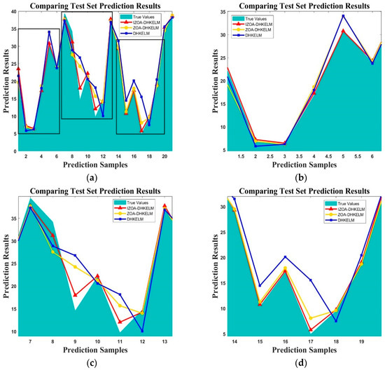
Figure 5.
Comparison of prediction and measured values for every model in the test set: (a) total overview; (b) Region b’s enlarged view; (c) Region c’s enlarged view; and (d) Region d’s enlarged view.
Figure 5 shows that, overall, the IZOA-DHKELM predicts the wood color closest to the actual value, which is better than the ZOA-DHKELM and DHKELMs. This indicates that the model has a high predictability. Local predictions from the IZOA-DHKELM are also closer to the actual values. Of the two models used as comparisons, the fit between the expected and actual values of the ZOA-DHKELM is slightly better than that of the DHKELM, and there is an important gap between DHKELM’s forecast and actual values. This indicates the value of optimizing the predictive model using the original heuristic algorithm.
Figure 6 shows the histogram of the prediction error of the IZOA-DHKELM. The error histogram visualizes the error between the predicted output and the target output. In the error histogram, the horizontal coordinate represents the error value, and the vertical coordinate represents the number of samples corresponding to the error value. Through the error histogram, we can see the error distribution at a glance, which can help us understand and solve the possible problems in the training course. As illustrated in the accompanying figure, the error histogram of the improved model does not show a skewed distribution, i.e., the number of samples on both sides of the zero value is not significantly different, which indicates that the model is well fitted and there is no overfitting or underfitting.
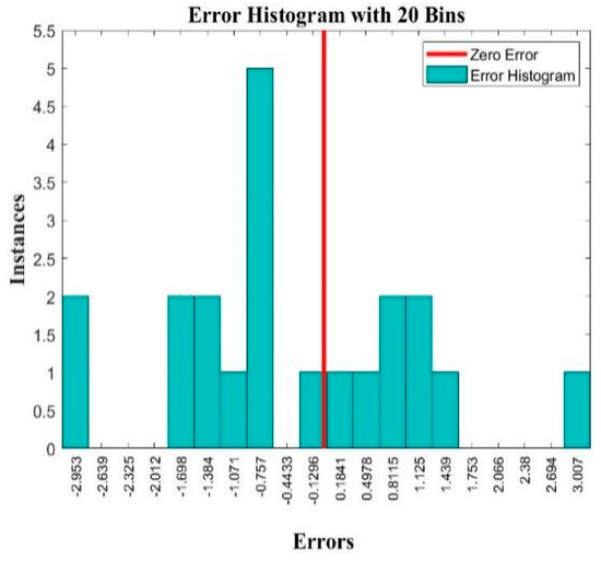
Figure 6.
The adaptation curves of the IZOA-DHKELM.
Figure 7 shows the error behavior of the IZOA-DHKELM on the training and test sets, including absolute and relative errors. The absolute error is the difference between the predicted and actual values, which can visualize the size of the prediction error. Relative error measures the difference between predicted and actual values, highlighting the size of the prediction error across various datasets. When evaluating the prediction model, the absolute error size and the relative error level should be considered, and the combination of the two is more effective. As you can see from Figure 8, in the training process, the IZOA-DHKELM demonstrates absolute and relative errors ranging between −5 and 5; in the testing process, the absolute error of the model is between −2.5 and 2.5, and the relative error is between −0.5 and 0.5, both of which are improved very significantly. The comparison between the training and testing processes shows that, after training, the error control of the IZOA-DHKELM is very impressive, and it is a more stable and trustworthy prediction model.
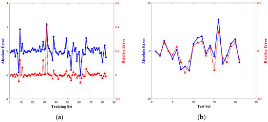
Figure 7.
The absolute and relative errors in the IZOA-DHKELM: (a) training set and (b) test set.
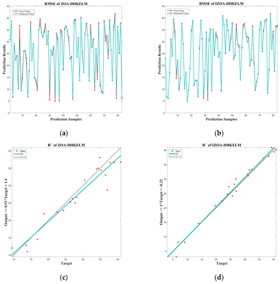
Figure 8.
Analytical plots of RMSE and R for the IZOA-DHKELM and ZOA-DHKELMs: (a) RMSE of ZOA-DHKELM; (b) RMSE of IZOA-DHKELM; (c) of ZOA-DHKELM; and (d) of IZOA-DHKELM.
4.3. Comparative Analysis of Model Performance
To confirm the effectiveness of the proposed IZOA-DHKELM in accurately predicting the color of heat-treated wood, further validation is required. This paper evaluates the model more accurately using four evaluation indexes. They are MAE, RMSE, MAPE, and . Detailed findings for each evaluation metric are presented in Table 3.
Table 3.
Evaluation indicators for each model.
The smaller the MAE, RMSE, and MAPE, the smaller the gap between the model’s predicted and actual values. This indicates that the higher the prediction accuracy of the model, the index of determination is generally between 0 and 1. The closer the value is to 1, the better the model’s predictions align with the actual outcomes, resulting in higher prediction accuracy. The table gives specific information about the various evaluation metrics for different models. The prediction performance of the DHKELM was enhanced to varying degrees by optimizing different metaheuristic algorithms. Nevertheless, the IZOA-DHKELM surpassed all other models in its ability to accurately forecast the color of heat-treated wood. The IZOA-DHKELM was evaluated against the ZOA-DHKELM. Its MAE, RMSE, and MAPE are reduced by 56.2%, 67.4%, and 34.2%, respectively. At the same time, is improved to 0.9952. This suggests that the IZOA has better tweaking features and can better optimize the DHKELM, thus making the IZOA-DHKELM more suitable for predicting the color of heat-treated wood. This paper highlights the effectiveness of three proposed improvements to ZOA, showcasing the dominance of the IZOA. Furthermore, it proves the IZOA-DHKELM’s superiority in accurately predicting the color of heat-treated wood. The number of parameters in a model significantly influences its predictive performance. Generally, a higher number of parameters enhances a model’s capability to process data effectively. In this article, we explore how the IZOA-DHKELM features more parameters than both the ZOA-DHKELM and DHKELMs, leading to improved outcomes. Notably, compared to the ZOA-DHKELM, the IZOA-DHKELM incorporates an additional escape factor “R”, and compared to the DHKELM, it adds specific parameters like and . These enhancements considerably boost the model’s predictive ability, highlighting the importance of parameter optimization for advanced data processing. In addition, Table 4 is a table of the comparative analysis of the IZOA-DHKELM with some published studies on the modeling of color changes during heat treatment of wood from the literature [11,35]. The results indicate that the IZOA-DHKELM outperforms several other models, showcasing significantly improved RMSE and (correlation coefficient) values. It is a trustworthy prediction model.
Table 4.
Performance comparison with published models.
Figure 8 shows the RMSE and analysis of the IZOA-DHKELM and ZOA-DHKELMs. (a) and (b) visualize the difference between the RMSE of the two models. (b) is well fitted and no significant difference between the true and predicted values occurs, while (a) shows substantial differences between the true and predicted values at multiple nodes. The IZOA-DHKELM demonstrates exceptional accuracy, and the ZOA-DHKELM shows poor precision in the prediction process. (c) and (d) are the analysis plots of the two models. It is clear from the plots that (c) has a much better fit; there are no obvious discrete points, and the relationship between predicted and actual values is very strong. In (d), there are multiple points with large deviations, and the fitting effect is reduced. Here, is mainly used to compare the performance of these two models on the same dataset, and it is obvious that the IZOA-DHKELM performs significantly better than the ZOA-DHKELM in this metric of and is more trustworthy.
The results of (a), (b), (c), and (d) reinforce the previous affirmation of the IZOA-DHKELM. In conclusion, the IZOA-DHKELM demonstrates outstanding performance in accurately predicting the color of heat-treated wood, making it a reliable choice for industry professionals.
5. Conclusions
In this paper, the IZOA-DHKELM was constructed to predict the color change in heat-treated wood. The main conclusions are as follows:
- As result of the research conducted, we obtained IZOA. First, IZOA’s global search capability is significantly better than ZOA’s. Second, IZOA’s search speed is adapted to the whole search process, which makes IZOA’s search efficiency significantly higher than ZOA’s. Finally, IZOA’s search accuracy is also higher than ZOA’s.
- The CEC test results reveal that IZOA exhibits a superior local unfolding ability compared to other models. It approaches the optimal solution more quickly and achieves faster convergence. In addition, the fitting accuracy of IZOA is significantly better than several different algorithms and maintains good accuracy and stability when solving high-dimensional problems.
- This study presents an innovative model for forecasting the performance of heat-treated wood. As the first of its kind, this model marks a significant advancement in the field. This is the innovation of this paper. Meanwhile, the results of the comparative analysis of model performance show that, in comparison with the model before improvement, the IZOA-DHKELM has the lowest MAE, RMSE, and MAPE and the highest . This shows that the prediction error of the IZOA-DHKELM is relatively small, and the prediction accuracy is relatively high. And it can better meet the performance requirements of heat-treated wood color prediction. In comparison with some published models for predicting the color change in heat-treated wood, the IZOA-DHKELM has the smallest RMSE and the largest . The model in this paper still has obvious performance advantages.
- However, there are some limitations to this study. Despite the fact that the proposed model has been shown to be superior to other algorithms in the color prediction of heat-treated wood by using metric measures and comparing different algorithms, there is still a lack of relevant statistical tests. The computational cost of adding the enhancements has not yet been analyzed, although IZOA significantly improves the optimization performance. In further research, we aim to continue to improve the model by comparing it with as many metaheuristics as possible. And we will also try to use the model to predict other properties of heat-treated wood, for example, mechanical properties and moisture content. This will help ensure that the model is used in a productive environment.
Author Contributions
Conceptualization, J.L. and W.W.; methodology, J.L.; software, J.L.; validation, J.L., Z.Q. and W.W.; formal analysis, J.L., Y.C. and W.W.; investigation, J.L., Z.Q., J.G. and W.W.; resources, J.L., Y.C. and W.W.; data curation, J.L., Y.C., Z.Q. and J.G.; writing—original draft preparation, J.L.; writing—review and editing, J.L.; visualization, J.L.; supervision, W.W.; project administration, W.W.; funding acquisition, W.W. All authors have read and agreed to the published version of the manuscript.
Funding
This research was supported by the Natural Scientific Foundation of Heilongjiang Province, grant number LC201407.
Data Availability Statement
The data presented in this study are available on request from the corresponding author.
Conflicts of Interest
The authors declare no conflicts of interest.
Appendix A
Table A1.
Color parameters of wood before heat treatment.
Table A1.
Color parameters of wood before heat treatment.
| Transverse | Radial | Tangential | |||||||
|---|---|---|---|---|---|---|---|---|---|
| Eucalypt | |||||||||
| Average | 54.1 | 7.4 | 15.7 | 63.8 | 8.0 | 19.9 | 61.5 | 8.5 | 18.9 |
| Minimum | 48.1 | 5.4 | 14.3 | 56.9 | 6.8 | 16.2 | 53.7 | 6.7 | 16.3 |
| Maximum | 63.6 | 9.6 | 20.3 | 67.4 | 10.1 | 23.0 | 69.9 | 11.7 | 30.4 |
| Standard deviation | 2.7 | 0.9 | 0.9 | 1.9 | 0.7 | 0.9 | 2.7 | 1.1 | 1.4 |
| Pinus pinaster | |||||||||
| Average | 76.1 | 6.9 | 24.1 | 74.3 | 7.6 | 23.3 | 67.3 | 7.2 | 16.3 |
| Minimum | 57.7 | 5.5 | 17.8 | 56.9 | 5.3 | 17.4 | 48.1 | 5.8 | 13.8 |
| Maximum | 80.4 | 9.1 | 27.6 | 78.7 | 11.4 | 28.5 | 72.0 | 8.7 | 19.6 |
| Standard deviation | 4.4 | 0.6 | 2.1 | 4.6 | 1.1 | 3.0 | 5.1 | 0.6 | 1.2 |
Table A2.
Changes in color parameters of heat-treated wood.
Table A2.
Changes in color parameters of heat-treated wood.
| Tree Species | Treatment Medium | Treatment Temperatures/℃ | Treatment Time/h | Profile Direction | /% | /% | |
|---|---|---|---|---|---|---|---|
| Eucalypt | Air | 170 | 2 | Tranv | −17.1 | 9.0 | −8.6 |
| Eucalypt | Air | 170 | 2 | Radial | −10.3 | 23.7 | −1.5 |
| Eucalypt | Air | 170 | 2 | Tang | −18.0 | 16.1 | −5.6 |
| Eucalypt | Air | 170 | 6 | Tranv | −27.9 | 7.8 | −15.5 |
| Eucalypt | Air | 170 | 6 | Radial | −25.0 | 17.3 | −9.1 |
| Eucalypt | Air | 170 | 6 | Tang | −35.0 | 10.9 | −19.7 |
| Eucalypt | Air | 170 | 12 | Tranv | −39.6 | −10.1 | −33.6 |
| Eucalypt | Air | 170 | 12 | Radial | −38.4 | 11.7 | −24.2 |
| Eucalypt | Air | 170 | 12 | Tang | −44.4 | −9.3 | −32.0 |
| Eucalypt | Air | 170 | 24 | Tranv | −45.5 | −8.4 | −35.1 |
| Eucalypt | Air | 170 | 24 | Radial | −50.1 | −5.6 | −40.4 |
| Eucalypt | Air | 170 | 24 | Tang | −50.8 | −4.0 | −37.4 |
| Eucalypt | Air | 180 | 2 | Tranv | −19.6 | 13.3 | −0.2 |
| Eucalypt | Air | 180 | 2 | Radial | −17.3 | 22.2 | −1.7 |
| Eucalypt | Air | 180 | 2 | Tang | −19.4 | 8.0 | −1.2 |
| Eucalypt | Air | 180 | 6 | Tranv | −38.7 | −18.9 | −37.4 |
| Eucalypt | Air | 180 | 6 | Radial | −38.3 | 12.4 | −19.6 |
| Eucalypt | Air | 180 | 6 | Tang | −43.3 | −1.9 | −33.3 |
| Eucalypt | Air | 180 | 12 | Tranv | −44.8 | −16.4 | −39.3 |
| Eucalypt | Air | 180 | 12 | Radial | −45.6 | 8.1 | −28.2 |
| Eucalypt | Air | 180 | 12 | Tang | −50.2 | −17.8 | −44.8 |
| Eucalypt | Air | 180 | 24 | Tranv | −51.5 | −28.3 | −54.1 |
| Eucalypt | Air | 180 | 24 | Radial | −51.7 | 1.1 | −42.1 |
| Eucalypt | Air | 180 | 24 | Tang | −55.6 | −35.0 | −69.5 |
| Eucalypt | Air | 190 | 2 | Tranv | −33.9 | 2.8 | −23.5 |
| Eucalypt | Air | 190 | 2 | Radial | −34.2 | 21.5 | −13.6 |
| Eucalypt | Air | 190 | 2 | Tang | −42.3 | 2.9 | −33.7 |
| Eucalypt | Air | 190 | 6 | Tranv | −45.6 | −26.2 | −45.6 |
| Eucalypt | Air | 190 | 6 | Radial | −49.3 | 1.2 | −37.3 |
| Eucalypt | Air | 190 | 6 | Tang | −51.2 | −22.4 | −56.9 |
| Eucalypt | Air | 190 | 12 | Tranv | −50.2 | −40.5 | −64.2 |
| Eucalypt | Air | 190 | 12 | Radial | −54.4 | −18.6 | −59.9 |
| Eucalypt | Air | 190 | 12 | Tang | −54.3 | −41.2 | −65.7 |
| Eucalypt | Air | 190 | 24 | Tranv | −50.8 | −29.2 | −58.4 |
| Eucalypt | Air | 190 | 24 | Radial | −56.3 | −37.0 | −70.1 |
| Eucalypt | Air | 190 | 24 | Tang | −55.3 | −40.8 | −72.2 |
| Eucalypt | Air | 200 | 2 | Tranv | −38.9 | −8.0 | −31.2 |
| Eucalypt | Air | 200 | 2 | Radial | −36.6 | 16.9 | −18.8 |
| Eucalypt | Air | 200 | 2 | Tang | −43.6 | −7.6 | −37.1 |
| Eucalypt | Air | 200 | 6 | Tranv | −50.5 | −49.6 | −67.9 |
| Eucalypt | Air | 200 | 6 | Radial | −51.6 | −13.5 | −46.7 |
| Eucalypt | Air | 200 | 6 | Tang | −56.0 | −38.7 | −69.8 |
| Eucalypt | Air | 200 | 12 | Tranv | −52.7 | −45.5 | −70.8 |
| Eucalypt | Air | 200 | 12 | Radial | −56.2 | −28.6 | −66.3 |
| Eucalypt | Air | 200 | 12 | Tang | −59.2 | −60.2 | −85.6 |
| Eucalypt | Vapor | 190 | 2 | Tranv | −41.7 | −4.9 | −38.4 |
| Eucalypt | Vapor | 190 | 2 | Radial | −41.6 | 10.2 | 10.2 |
| Eucalypt | Vapor | 190 | 2 | Tang | −36.6 | 10.5 | −22.7 |
| Eucalypt | Vapor | 190 | 6 | Tranv | −43.8 | −6.2 | −37.7 |
| Eucalypt | Vapor | 190 | 6 | Radial | −47.0 | 2.8 | 2.8 |
| Eucalypt | Vapor | 190 | 6 | Tang | −45.5 | 6.6 | −33.4 |
| Eucalypt | Vapor | 190 | 12 | Tranv | −44.0 | −14.5 | −45.7 |
| Eucalypt | Vapor | 190 | 12 | Radial | −46.0 | −4.0 | −4.0 |
| Eucalypt | Vapor | 190 | 12 | Tang | −44.8 | −4.0 | −36.5 |
| Eucalypt | Vapor | 200 | 2 | Tranv | −36.5 | 3.5 | −25.9 |
| Eucalypt | Vapor | 200 | 2 | Radial | −36.3 | 9.7 | −24.6 |
| Eucalypt | Vapor | 200 | 2 | Tang | −37.2 | 16.1 | −22.2 |
| Eucalypt | Vapor | 200 | 6 | Tranv | −50.7 | −16.1 | −50.3 |
| Eucalypt | Vapor | 200 | 6 | Radial | −51.6 | −13.0 | −52.6 |
| Eucalypt | Vapor | 200 | 6 | Tang | −52.7 | −7.7 | −46.6 |
| Eucalypt | Vapor | 200 | 12 | Tranv | −51.5 | −39.0 | −62.9 |
| Eucalypt | Vapor | 200 | 12 | Radial | −54.4 | −23.1 | −58.6 |
| Eucalypt | Vapor | 200 | 12 | Tang | −54.1 | −26.1 | −58.4 |
| Eucalypt | Vapor | 210 | 2 | Tranv | −49.6 | −21.7 | −43.9 |
| Eucalypt | Vapor | 210 | 2 | Radial | −50.4 | −7.5 | −43.7 |
| Eucalypt | Vapor | 210 | 2 | Tang | −49.0 | −22.5 | −45.8 |
| Eucalypt | Vapor | 210 | 6 | Tranv | −53.1 | −42.5 | −64.8 |
| Eucalypt | Vapor | 210 | 6 | Radial | −54.7 | −33.9 | −62.9 |
| Eucalypt | Vapor | 210 | 6 | Tang | −55.8 | −39.0 | −64.4 |
| Eucalypt | Vapor | 210 | 12 | Tranv | −54.5 | −53.2 | −72.7 |
| Eucalypt | Vapor | 210 | 12 | Radial | −56.8 | −38.0 | −67.8 |
| Eucalypt | Vapor | 210 | 12 | Tang | −56.7 | −38.3 | −63.5 |
| Pinus pinaster | Air | 170 | 2 | Tranv | −9.4 | −12.4 | 19.5 |
| Pinus pinaster | Air | 170 | 2 | Radial | −10.5 | 22.8 | 12.2 |
| Pinus pinaster | Air | 170 | 2 | Tang | −12.8 | 26.5 | 22.7 |
| Pinus pinaster | Air | 170 | 6 | Tranv | −19.0 | −5.9 | 25.1 |
| Pinus pinaster | Air | 170 | 6 | Radial | −17.7 | 48.3 | 14.7 |
| Pinus pinaster | Air | 170 | 6 | Tang | −20.7 | 41.7 | 27.1 |
| Pinus pinaster | Air | 170 | 12 | Tranv | −25.2 | −7.9 | 31.5 |
| Pinus pinaster | Air | 170 | 12 | Radial | −28.7 | 83.3 | 14.7 |
| Pinus pinaster | Air | 170 | 12 | Tang | −52.4 | 20.6 | −21.6 |
| Pinus pinaster | Air | 170 | 24 | Tranv | −32.1 | 11.5 | 31.8 |
| Pinus pinaster | Air | 170 | 24 | Radial | −44.7 | 87.2 | −6.5 |
| Pinus pinaster | Air | 170 | 24 | Tang | −45.3 | 71.5 | −8.0 |
| Pinus pinaster | Air | 180 | 2 | Tranv | −15.2 | −0.7 | 24.9 |
| Pinus pinaster | Air | 180 | 2 | Radial | −14.1 | 27.7 | 12.2 |
| Pinus pinaster | Air | 180 | 2 | Tang | −19.4 | 55.5 | 23.7 |
| Pinus pinaster | Air | 180 | 6 | Tranv | −24.3 | 7.4 | 38.3 |
| Pinus pinaster | Air | 180 | 6 | Radial | −34.7 | 83.2 | 11.1 |
| Pinus pinaster | Air | 180 | 6 | Tang | −32.8 | 72.9 | 19.2 |
| Pinus pinaster | Air | 180 | 12 | Tranv | −36.1 | 18.7 | 27.8 |
| Pinus pinaster | Air | 180 | 12 | Radial | −44.3 | 77.2 | −6.4 |
| Pinus pinaster | Air | 180 | 12 | Tang | −47.0 | 76.6 | −8.7 |
| Pinus pinaster | Air | 180 | 24 | Tranv | −40.5 | 32.1 | 29.1 |
| Pinus pinaster | Air | 180 | 24 | Radial | −52.5 | 66.9 | −27.2 |
| Pinus pinaster | Air | 180 | 24 | Tang | −52.1 | 37.8 | −35.0 |
| Pinus pinaster | Air | 190 | 2 | Tranv | −19.4 | −6.4 | 27.1 |
| Pinus pinaster | Air | 190 | 2 | Radial | −23.9 | 70.3 | 21.9 |
| Pinus pinaster | Air | 190 | 2 | Tang | −25.7 | 66.2 | 26.8 |
| Pinus pinaster | Air | 190 | 6 | Tranv | −32.8 | 14.1 | 33.4 |
| Pinus pinaster | Air | 190 | 6 | Radial | −43.1 | 79.4 | −4.4 |
| Pinus pinaster | Air | 190 | 6 | Tang | −38.1 | 72.5 | 15.9 |
| Pinus pinaster | Air | 190 | 12 | Tranv | −45.4 | 12.3 | −0.9 |
| Pinus pinaster | Air | 190 | 12 | Radial | −57.4 | 52.4 | −43.8 |
| Pinus pinaster | Air | 190 | 12 | Tang | −56.3 | 39.0 | −45.8 |
| Pinus pinaster | Air | 190 | 24 | Tranv | −49.4 | 8.1 | −20.7 |
| Pinus pinaster | Air | 190 | 24 | Radial | −58.5 | 30.8 | −53.2 |
| Pinus pinaster | Air | 190 | 24 | Tang | −58.8 | 14.6 | −57.8 |
| Pinus pinaster | Air | 200 | 2 | Tranv | −28.4 | −0.8 | 31.2 |
| Pinus pinaster | Air | 200 | 2 | Radial | −35.3 | 87.4 | 2.6 |
| Pinus pinaster | Air | 200 | 2 | Tang | −33.9 | 64.8 | 12.2 |
| Pinus pinaster | Air | 200 | 6 | Tranv | −44.6 | 9.7 | 3.1 |
| Pinus pinaster | Air | 200 | 6 | Radial | −52.1 | 68.6 | −28.2 |
| Pinus pinaster | Air | 200 | 6 | Tang | −54.0 | 40.3 | −38.1 |
| Pinus pinaster | Air | 200 | 12 | Tranv | −52.9 | 4.9 | −25.2 |
| Pinus pinaster | Air | 200 | 12 | Radial | −59.5 | 38.8 | −49.4 |
| Pinus pinaster | Air | 200 | 12 | Tang | −60.4 | 3.3 | −63.4 |
| Pinus pinaster | Vapor | 190 | 2 | Tranv | −19.2 | 82.4 | 42.2 |
| Pinus pinaster | Vapor | 190 | 2 | Radial | −38.6 | 33.5 | −9.7 |
| Pinus pinaster | Vapor | 190 | 2 | Tang | −24.4 | 52.3 | 13.1 |
| Pinus pinaster | Vapor | 190 | 6 | Tranv | −28.1 | 63.1 | 26.7 |
| Pinus pinaster | Vapor | 190 | 6 | Radial | −41.2 | 33.6 | −12.4 |
| Pinus pinaster | Vapor | 190 | 6 | Tang | −34.6 | 94.0 | 19.1 |
| Pinus pinaster | Vapor | 190 | 12 | Tranv | −29.9 | 70.3 | 32.4 |
| Pinus pinaster | Vapor | 190 | 12 | Radial | −40.3 | 30.9 | −13.6 |
| Pinus pinaster | Vapor | 190 | 12 | Tang | −34.8 | 78.6 | 5.7 |
| Pinus pinaster | Vapor | 200 | 2 | Tranv | −20.3 | 51.6 | 33.7 |
| Pinus pinaster | Vapor | 200 | 2 | Radial | −37.6 | 25.4 | −6.3 |
| Pinus pinaster | Vapor | 200 | 2 | Tang | −30.3 | 37.4 | 2.6 |
| Pinus pinaster | Vapor | 200 | 6 | Tranv | −30.7 | 64.1 | 21.4 |
| Pinus pinaster | Vapor | 200 | 6 | Radial | −43.4 | 42.0 | −11.1 |
| Pinus pinaster | Vapor | 200 | 6 | Tang | −37.3 | 62.9 | −0.5 |
| Pinus pinaster | Vapor | 200 | 12 | Tranv | −34.1 | 59.9 | 18.3 |
| Pinus pinaster | Vapor | 200 | 12 | Radial | −45.2 | 43.1 | −13.6 |
| Pinus pinaster | Vapor | 200 | 12 | Tang | −39.8 | 54.5 | −5.0 |
| Pinus pinaster | Vapor | 210 | 2 | Tranv | −34.6 | 50.7 | 11.0 |
| Pinus pinaster | Vapor | 210 | 2 | Radial | −44.8 | 48.0 | −16.8 |
| Pinus pinaster | Vapor | 210 | 2 | Tang | −40.0 | 83.0 | 0.9 |
| Pinus pinaster | Vapor | 210 | 6 | Tranv | −39.5 | 66.6 | 9.8 |
| Pinus pinaster | Vapor | 210 | 6 | Radial | −52.9 | 40.4 | −30.7 |
| Pinus pinaster | Vapor | 210 | 6 | Tang | −47.6 | 54.6 | −13.5 |
| Pinus pinaster | Vapor | 210 | 12 | Tranv | −40.8 | 56.2 | 9.0 |
| Pinus pinaster | Vapor | 210 | 12 | Radial | −50.9 | 44.3 | −21.9 |
| Pinus pinaster | Vapor | 210 | 12 | Tang | −47.5 | 49.6 | −17.7 |
References
- Esteves, B.; Ferreira, H.; Viana, H.; Ferreira, J.; Domingos, I.; Cruz-Lopes, L.; Jones, D.; Nunes, L. Termite Resistance, Chemical and Mechanical Characterization of Paulownia tomentosa Wood before and after Heat Treatment. Forests 2021, 12, 1114. [Google Scholar] [CrossRef]
- Jirouš-Rajković, V.; Miklečić, J. Heat-Treated Wood as a Substrate for Coatings, Weathering of Heat-Treated Wood, and Coating Performance on Heat-Treated Wood. Adv. Mater. Sci. Eng. 2019, 2019, 8621486. [Google Scholar] [CrossRef]
- Liu, M.; Zhang, L.; Chen, J.; Chen, S.; Lei, Y.; Chen, Z.; Yan, L. Response relationships between the color parameters and chemical compositions of heat-treated wood. Holzforschung 2024, 78, 387–401. [Google Scholar] [CrossRef]
- Borůvka, V.; Šedivka, P.; Novák, D.; Holeček, T.; Turek, J. Haptic and Aesthetic Properties of Heat-Treated Modified Birch Wood. Forests 2021, 12, 1081. [Google Scholar] [CrossRef]
- Sikora, A.; Kačík, F.; Gaff, M.; Vondrová, V.; Bubeníková, T.; Kubovský, I. Impact of thermal modification on color and chemical changes of spruce and oak wood. J. Wood Sci. 2018, 64, 406–416. [Google Scholar] [CrossRef]
- Aydemir, D.; Gunduz, G.; Ozden, S. The influence of thermal treatment on color response of wood materials. Color Res. Appl. 2012, 37, 148–153. [Google Scholar] [CrossRef]
- Jiang, H.; Lu, Q.; Li, G.; Li, M.; Li, J. Effect of heat treatment on the surface color of rubber wood (Hevea brasiliensis). Wood Res. 2020, 65, 633–644. [Google Scholar] [CrossRef]
- Jin, T.; Kang, C.W.; Lee, N.H.; Kang, H.Y.; Matsumura, J. Changes in the color and physical properties of wood by high temperature heat treatment. J. Fac. Agric. Kyushu Univ. 2011, 56, 129–137. [Google Scholar] [CrossRef]
- Yixing, L.; Jian, L.; Jinman, W.; Jinsong, Y.; Yanhua, M. The effect of heat treatment on different species wood colour. J. Northeast. For. Univ. 1994, 5, 73–78. [Google Scholar] [CrossRef]
- Chen, Y.; Fan, Y.; Gao, J.; Stark, N.M. The effect of heat treatment on the chemical and color change of black locust (Robinia pseudoacacia) wood flour. BioResources 2012, 7, 1157–1170. [Google Scholar] [CrossRef]
- Haftkhani, A.R.; Abdoli, F.; Sepehr, A.; Mohebby, B. Regression and ANN models for predicting MOR and MOE of heat-treated fir wood. J. Build. Eng. 2021, 42, 102788. [Google Scholar] [CrossRef]
- Van Nguyen, T.H.; Nguyen, T.T.; Ji, X.; Guo, M. Predicting color change in wood during heat treatment using an artificial neural network model. BioResources 2018, 13, 6250–6264. [Google Scholar] [CrossRef]
- Li, J.; Li, N.; Li, J.; Wang, W.; Wang, H. Prediction of thermally modified wood color change after artificial weathering based on IPSO-SVM model. Forests 2023, 14, 948. [Google Scholar] [CrossRef]
- Mo, J.; Tamboli, D.; Haviarova, E. Prediction of the color change of surface thermally treated wood by artificial neural network. Eur. J. Wood Wood Prod. 2023, 81, 1135–1146. [Google Scholar] [CrossRef]
- Li, W.; Wang, X.; Tang, M. A transformer fault diagnosis method based on EHBA-DHKELM-Adaboost model. J. Intell. Fuzzy Syst. 2024, 46, 1–13. [Google Scholar] [CrossRef]
- Yan, H. Short-term Photovoltaic Power Prediction based on ICEEMDAN and Optimized Deep Hybrid Kernel Extreme Learning Machine. Int. J. Mech. Electr. Eng. 2024, 2, 32–46. [Google Scholar] [CrossRef]
- Wang, W.; Cui, X.; Qi, Y.; Xue, K.; Wang, H.; Bai, C. Prediction model of coal seam gas content based on kernel principal component analysis and IDBO-DHKELM. Meas. Sci. Technol. 2024, 35, 115113. [Google Scholar] [CrossRef]
- Wang, J.; Lu, S.; Wang, S.H.; Zhang, Y. A review on extreme learning machine. Multimed. Tools Appl. 2022, 81, 41611–41660. [Google Scholar] [CrossRef]
- Liu, X.; Wang, L.; Huang, G.B.; Zhang, J.; Yin, J. Multiple kernel extreme learning machine. Neurocomputing 2015, 149, 253–264. [Google Scholar] [CrossRef]
- Qiao, L.; Chen, L.; Li, Y.; Hua, W.; Wang, P. Predictions of Aeroengines’ Infrared Radiation Characteristics Based on HKELM Optimized by the Improved Dung Beetle Optimizer. Sensors 2024, 24, 1734. [Google Scholar] [CrossRef]
- Tschannen, M.; Bachem, O.; Lucic, M. Recent advances in autoencoder-based representation learning. arXiv 2018, arXiv:1812.05069. [Google Scholar]
- Trojovská, E.; Dehghani, M.; Trojovský, P. Zebra optimization algorithm: A new bio-inspired optimization algorithm for solving optimization algorithm. IEEE Access 2022, 10, 49445–49473. [Google Scholar] [CrossRef]
- Xue, J.; Shen, B. A novel swarm intelligence optimization approach: Sparrow search algorithm. Syst. Sci. Control. Eng. 2020, 8, 22–34. [Google Scholar] [CrossRef]
- Kennedy, J.; Eberhart, R. Particle swarm optimization. In Proceedings of the ICNN'95-International Conference on Neural Networks, Perth, WA, Australia, 27 November–1 December 1995; IEEE: Piscataway, NJ, USA, 1995; Volume 4, pp. 1942–1948. [Google Scholar]
- Esteves, B.; Velez Marques, A.; Domingos, I.; Pereira, H. Heat-induced colour changes of pine (pinus pinaster) and eucalypt (Eucalyptus globulus) wood. Wood Sci. Technol. 2008, 42, 369–384. [Google Scholar] [CrossRef]
- Panda, S.K.; Jana, P.K. Efficient task scheduling algorithms for heterogeneous multi-cloud environment. J. Supercomput. 2015, 71, 1505–1533. [Google Scholar] [CrossRef]
- Despagne, F.; Massart, D.L. Neural networks in multivariate calibration. Analyst 1998, 123, 157R–178R. [Google Scholar] [CrossRef]
- Mitsui, K.; Takada, H.; Sugiyama, M.; Hasegawa, R. Changes in the properties of light-irradiated wood with heat treatment. Part 1. Effect of treatment conditions on the change in color. Holzforschung 2001, 55, 601–605. [Google Scholar] [CrossRef]
- Chopra, N.; Ansari, M.M. Golden jackal optimization: A novel nature-inspired optimizer for engineering applications. Expert Syst. Appl. 2022, 198, 116924. [Google Scholar] [CrossRef]
- Dehghani, M.; Hubálovský, Š.; Trojovský, P. Northern goshawk optimization: A new swarm-based algorithm for solving optimization problems. IEEE Access 2021, 9, 162059–162080. [Google Scholar] [CrossRef]
- Mirjalili, S.; Mirjalili, S.M.; Lewis, A. Grey wolf optimizer. Adv. Eng. Softw. 2014, 69, 46–61. [Google Scholar] [CrossRef]
- Hashim, F.A.; Houssein, E.H.; Hussain, K.; Mabrouk, M.S.; Al-Atabany, W. Honey Badger Algorithm: New metaheuristic algorithm for solving optimization problems. Math. Comput. Simul. 2022, 192, 84–110. [Google Scholar] [CrossRef]
- Zhang, X.; Kano, M.; Matsuzaki, S. A comparative study of deep and shallow predictive techniques for hot metal temperature prediction in blast furnace ironmaking. Comput. Chem. Eng. 2019, 130, 106575. [Google Scholar] [CrossRef]
- Yao, X.; Liu, Y.; Lin, G. Evolutionary programming made faster. IEEE Trans. Evol. Comput. 1999, 3, 82–102. [Google Scholar]
- Nguyen, T.T.; Van Nguyen, T.H.; Ji, X.; Yuan, B.; Trinh, H.M.; Do, K.T.L.; Guo, M. Prediction of the color change of heat-treated wood during artificial weathering by artificial neural network. Eur. J. Wood Wood Prod. 2019, 77, 1107–1116. [Google Scholar] [CrossRef]
Disclaimer/Publisher’s Note: The statements, opinions and data contained in all publications are solely those of the individual author(s) and contributor(s) and not of MDPI and/or the editor(s). MDPI and/or the editor(s) disclaim responsibility for any injury to people or property resulting from any ideas, methods, instructions or products referred to in the content. |
© 2025 by the authors. Licensee MDPI, Basel, Switzerland. This article is an open access article distributed under the terms and conditions of the Creative Commons Attribution (CC BY) license (https://creativecommons.org/licenses/by/4.0/).