Abstract
Carbon utilization efficiency (CUE) in terrestrial ecosystems stands as a pivotal metric for assessing ecosystem functionality. Investigating the spatiotemporal dynamics of regional CUE within the context of global climate change not only provides a theoretical foundation for understanding terrestrial carbon cycling but also furnishes essential data support for formulating sustainable management strategies at a regional scale. This study focuses on the southeastern region of Tibet. Utilizing monthly and yearly MOD17A2HGF as primary sources, we employ Thiel–Sen estimation and Mann–Kendall trend analysis to scrutinize the spatiotemporal dynamics of CUE. Systematic analysis of the stability of CUE spatiotemporal changes in the Southeast Tibet region is conducted using the coefficient of variation analysis. The Hurst model is then applied to prognosticate future CUE changes in Southeast Tibet. Additionally, a comprehensive analysis of CUE is undertaken by integrating meteorological data and land-use data. The findings reveal the following: (1) At the monthly scale, regional CUE exhibits discernible variations synchronized with the growth season, with different vegetation types displaying diverse fluctuation patterns. The high-altitude forest area manifests the least annual CUE fluctuations, while evergreen needleleaf forests and evergreen broadleaf forests demonstrate larger variations. At the yearly scale, CUE reveals a non-significant upward trend overall, but there is an augmented fluctuation observed from 2019 to 2022. (2) CUE in Southeast Tibet demonstrates sensitivity to temperature and precipitation variations, with temperature exhibiting a more pronounced and strongly correlated impact, especially in Gongjo County and Qamdo Town. Temperature and precipitation exert opposing influences on CUE changes in the Southeast Tibet region. In the southern (below 28° N) and northern (above 31° N) regions of Southeast Tibet, the response of CUE to temperature and precipitation variations differs. Moreover, over 62.3% of the areas show no sustained trend of change. (3) Vegetation type emerges as a principal factor determining the scope and features of vegetation CUE changes. Grassland and sparse grassland areas exhibit markedly higher CUE values than evergreen broadleaf forests, deciduous broadleaf forests, evergreen needleleaf forests, and deciduous needleleaf forests. Notably, the CUE fluctuation in shrublands and areas with embedded farmland vegetation surpasses that of other vegetation types.
1. Introduction
The heightened impacts of global climatic variability have underscored the significance of the global carbon cycle in climate change research [1,2,3]. Forest ecosystems, as the predominant component and the largest carbon reservoir within terrestrial ecosystems, contribute approximately two-thirds of the terrestrial carbon involved in restoration initiatives [4,5,6,7]. This contribution assumes a crucial role in modulating the global carbon equilibrium and alleviating the escalation of greenhouse gas concentrations. Consequently, it is imperative to quantify the spatiotemporal distribution patterns of forest carbon reservoirs and elucidate the characteristics of regional carbon pools.
In recent academic discourse, researchers have extensively explored the estimation methodologies of carbon reservoirs. Traditional methods for estimating regional-scale carbon sinks primarily involve plot inventories, biomass models, micrometeorology, and integrated observations [8,9,10,11]. Strohbach et al. [12] employed the carbon footprint methodology to conduct a rigorous statistical analysis of the carbon sink capacity in newly established green spaces situated in Leipzig, Germany. Pan et al. [13] undertook a thorough and extended analysis of carbon sequestration in global forests, employing forest inventory data and advancing ecosystem carbon research over an extended temporal horizon. Fang et al. [14] implemented biomass models to evaluate fluctuations in China’s forest carbon reservoirs, mean carbon density, and carbon source–sink dynamics spanning the previous five decades. They formulated a comprehensive carbon cycling model for terrestrial ecosystems in China. Wu et al. [15] employed the method of continuous functions utilizing biomass conversion factors to ascertain the vegetation carbon stock within China’s natural forest reserves. Conventional methodologies frequently fall short in delineating the spatial distribution of vegetation carbon reservoirs, limiting their capability to discern the carbon sink status of an ecosystem solely based on aggregate quantities. Comprehensive, streamlined, expeditious, and precise methodologies for discerning carbon sinks are still in the nascent stages of advancement. In conjunction with the advancement of remote sensing techniques and advancements in geographic information technology (GIS), the pervasive integration of remote sensing datasets into models for estimating carbon sink dynamics has become prevalent. Vegetative Net Primary Productivity (NPP) is defined as the disparity between the overall Gross Primary Productivity (GPP) [16,17,18] of vegetation and autotrophic respiration (Ra). Here, Ra signifies the carbon quantity lost due to plant respiration, encompassing both plant growth respiration (Rg) and maintenance respiration (Rm). This parameter serves as a targeted descriptor for characterizing the carbon sequestration capacity of forest ecosystems. GPP [19,20], regarded as a pivotal parameter in carbon cycle investigations, accentuates the significance of vegetation in the context of carbon sequestration. This fundamental variable serves as a key indicator of the photosynthetic carbon assimilation capacity of ecosystems, contributing essential insights into their potential as carbon sinks. CUE, delineated as the quotient of NPP to GPP, emerges as a critical metric for assessing the carbon sequestration capacity of ecosystems. A higher CUE signifies a more robust carbon assimilation capacity and greater potential for carbon sequestration, contributing to carbon stability and long-term retention. Therefore, examining the variation and impact of ecosystem vegetation CUE is indispensable for evaluating the carbon sequestration capacity of regional ecosystems and devising management strategies to enhance the long-term carbon storage potential of ecosystems.
Numerous scholars have conducted research on CUE in forest ecosystems at different temporal and spatial scales, revealing variations in CUE across these scales. The spatiotemporal characteristics of forest CUE are influenced by multiple factors, including temperature, precipitation, intrinsic conditions, environmental conditions (such as altitude and climate), and human activities (such as logging) [21]. Various factors exhibit differential impacts on CUE at different spatial scales, and the factors influencing forest ecosystem CUE often change with variations in temporal scales [22,23,24]. Existing studies indicate that forest CUE generally fluctuates between 0.20 and 0.83 [25]. At the spatial scale, forest ecosystem CUE tends to be higher in high-latitude regions [26]. The variation in CUE along longitudinal lines is more pronounced, and it is positively correlated with altitude. At the temporal scale, the average CUE of forest ecosystems follows a pattern of spring > summer > autumn [27]. As a function related to productivity and respiration, forest CUE is influenced by a combination of both biotic and abiotic factors [28]. In summary, the spatiotemporal characteristics of forest CUE necessitate region-specific and time-specific research. There is existing research on the variability of forest CUE, with microanalytical methods (quantitative studies on regional CUE effects of CO2 fertilization and land use [29]) being more widespread. However, there is a scarcity of studies employing remote sensing to analyze CUE in Southeast Tibet, and the spatiotemporal analysis of CUE in this region is largely unexplored.
The Qinghai–Tibet Plateau, recognized as the “Third Pole” and the “Roof of the World”, is the youngest and highest plateau (3000–5000 m) globally [30]. Due to its high elevation, the Qinghai–Tibet Plateau is one of the most crucial and sensitive regions to climate and precipitation changes [31]. Research indicates that over the past 600 years [32], each warming and cooling phase in China first occurred on the plateau. The temperature on the plateau rises faster compared to other regions. Owing to its lower temperatures and slower decomposition rates, the plateau’s soils contain substantial amounts of soil organic carbon. The increase in temperature and carbon dioxide concentration can enhance NPP in certain areas. Tibet, comprising the southeastern part of the Qinghai–Tibet Plateau, is one of China’s five major forested regions. The southeastern Tibetan region, characterized by pristine forests, encompasses a variety of forest vegetation ranging from tropical and subtropical to cold temperate climates, with both humid and semi-humid conditions. This geographical expanse encompasses a diverse array of needleleaf and broadleaf tree species, spanning from subtropical to cold temperate zones. Such distribution renders the area a paradigmatic representation of biodiversity, distinguishing it as one of the most notable regions in China and globally. Investigating the CUE of forests in Southeastern Tibet is of significant importance for understanding forest carbon sequestration capabilities, comprehending carbon cycle mechanisms, protecting the ecological environment, and formulating climate change strategies [33].
Building upon the aforementioned, this study utilizes MODIS GPP and MODIS PSNnet satellite imagery analysis data. The research focuses on the southeastern Tibetan region, specifically the Nyingchi and Qamdo areas. By utilizing remote sensing imagery and temperature, precipitation, and land-use data from 2012 to 2022, combined with path analysis, the study investigates the spatiotemporal distribution characteristics of vegetation CUE over the past 11 years and its influencing factors. The research outcomes contribute to a deeper understanding of the spatiotemporal features of vegetation CUE in forested areas, along with the response levels to various factors. Moreover, the investigation furnishes a scientific underpinning for advancing the carbon-neutralization potential of ecosystems within sylvan locales.
2. Materials and Methods
2.1. Overview of the Study Area
In the northern part of Nyingchi City, the landscape is characterized by the Nyainqentanglha Mountains to the north, the eastern section of the Himalayas to the south, the residual range of the Gangdise Mountains to the northwest, and the Hengduan Mountains to the east. The primary mountain ranges exhibit an east–west orientation for the first three, while the latter predominantly follows a north–south trajectory. Elevations exceeding 4800 m showcase a prevalence of contemporary glacial and snowy landforms. The region situated between 3800 and 4800 m is characterized by permafrost and periglacial landforms. Areas below 3800 m are primarily shaped by fluvial erosion and accumulation landforms, accompanied by the extensive development of various physical landform processes such as gravity and debris flows. The profound elevation differentials within the area give rise to a distinct vertical zoning phenomenon, where different elevation zones manifest various geomorphic types and their combinations in both vertical and horizontal dimensions.
The southern part of Nyingchi City, in proximity to the Indian Ocean, experiences an oceanic monsoon climate marked by relatively minor climatic variations and favorable thermal conditions. The Himalayas play a crucial role in intercepting substantial warm and humid air currents originating from the Bay of Bengal and the Indian Ocean. Notably, the vertical climate zones on the southern and northern slopes exhibit discernible disparities. On the southern slope, elevation change corresponds to a sequence of five distinct climate zones, namely tropical, subtropical, warm temperate, temperate, and sub-frigid zones. Conversely, the northern slope, situated within the plateau interior and characterized by lower moisture levels, exhibits a simpler spectrum of vertical climate zones. The temperate zone on the northern slope is further subdivided into warm, moderate, and cool subzones. Additionally, three dry–wet type areas—humid, semi-humid, and semi-arid climate regions—are identified. Classifying Nyingchi based on thermal levels, dry–wet types, and geomorphic distinctions yields categories such as mountainous tropical, subtropical humid canyon agroforestry climate region; plateau temperate humid, semi-humid, semi-arid river valley basin agroforestry climate region; eastern temperate, sub-frigid humid high-altitude forest climate region; and central sub-frigid, frigid semi-humid, humid high-altitude meadow desert climate region. This classification results in five primary climate regions and four sub-regions [34].
Nyingchi City showcases a diverse array of vegetation types, encompassing tropical, subtropical, temperate, and alpine cold zones. The distribution of vegetation types is characterized not only by horizontal zoning but also by distinct vertical zoning. The primary vegetation types include sparse alpine cushion vegetation, alpine and subalpine meadow and shrub meadow vegetation, dark coniferous forests dominated by spruce and fir, light coniferous forests dominated by high-mountain pine and Yunnan pine, Tibetan cypress and sparse forest of giant cypress, evergreen broadleaf forests dominated by high-mountain oak, deciduous broadleaf forests dominated by poplar and birch, subtropical broadleaf forests with mixed evergreen and deciduous broadleaf trees, tropical mountain evergreen rainforests and tropical seasonal rainforests, river valley meadows, shrubs, and shrub grasslands.
Chamdo City is situated in the eastern part of the Tibet Autonomous Region, upstream of the Lancang River, serving as the eastern gateway to the autonomous region. Located between 93°6′ and 99°2′ east longitude and 28°5′ and 32°6′ north latitude, Chamdo is situated in proximity to Degé, Baiyu, Shiqu, and Batang counties in the eastern sector of Sichuan Province, demarcated by a river. Additionally, it shares boundaries with Deqin County in Yunnan Province to the southeast, Nyingchi City to the southwest, Nagqu City to the northwest, and Yushu Tibetan Autonomous Prefecture in Qinghai Province to the north. Encompassing a total expanse of 109.83 thousand square kilometers, Chamdo constitutes 8.9% of the overall territory of the Tibet Autonomous Region.
Chamdo City experiences a plateau subtropical sub-humid climate, characterized by sub-frigid conditions in the northwest and north, and mild and humid conditions in the southeast. The region is subject to prolonged sunshine hours with distinct dry and wet seasons. The annual average temperature is approximately 7.6 °C, and the annual precipitation ranges from 400 to 600 mm. These climatic attributes reflect the typical characteristics of a plateau climate.
The Chamdo region boasts a rich abundance of forest resources, securing its position as Tibet’s second-largest forested area, encompassing a current forested expanse of 1.42 million hectares. The shrub forest spans 217,800 hectares, contributing to a forest coverage rate of 31.71%, with a voluminous wood stock totaling 3.64 billion cubic meters. Noteworthy dark coniferous species in Chamdo City include spruce, fir, high-mountain pine, Chinese oil pine, big-cone red pine, and Chinese hemlock. Mixed coniferous and broadleaf forests feature species such as Chinese white poplar, Chinese aspen, birch, Sino-Douglas fir, big-cone spruce, maple, walnut, spruce, and high-mountain pine. Additionally, shrub forests showcase species like high-mountain willow, three-needle pine, Rhododendron anthopogon, Japanese kerria, and creeping juniper.
The hydrological system in Chamdo City aligns with an external drainage system, encompassing major rivers like the Nu River, Lancang River, Jinsha River, and their tributaries. This region serves as a confluence area for the upper reaches of significant rivers in Southeast Asia and China, ultimately draining into the Pacific and Indian Ocean basins. The Nu River constitutes the upper reaches of the Salween River, part of the Indian Ocean basin. The Lancang River and Jinsha River belong to the Pacific Ocean basin, with the Jinsha River serving as the upper reaches of the Yangtze River, concluding in the East China Sea, and the Lancang River constituting the upper reaches of the Mekong River, traversing the Hengduan Mountains before reaching the South China Sea.
Concerning land resources in Chamdo City, the overall landscape is characterized by grassland dominance over forested land, with certain parcels temporarily deemed unsuitable for utilization. The aggregate land area in the region extends to 16.301 million mu (approximately 10.867 million hectares), with grassland encompassing 8.433 million mu (approximately 5.622 million hectares), constituting 51.74% of the total land resource area. Predominantly natural grassland, only 31% is distributed within valleys below 3700 m in altitude, while the remaining 69% is situated on the plateau at elevations between 3700 and 4300 m. Cultivated land occupies 25.7% of the total land area. Additionally, land temporarily unsuitable for agriculture, animal husbandry, and forestry accounts for 19.7% of the total land resource area, featuring barren rock, sandy areas, and gravelly terrain. Some of these plots, located at high altitudes, pose significant challenges for development, rendering them impractical for improvement and utilization.
2.2. Data and Methods
2.2.1. MODIS GPP and PSNnet
This study utilizes the MODIS product dataset (MOD17A2HGF) from the years 2012 to 2022, obtained from the NASA website (https://ladsweb.modaps.eosdis.nasa.gov) (accessed on 27 October 2023) [35]. The dataset possesses a temporal granularity of 8 days and a spatial precision of 500 m.
The dataset facilitates persistent global surveillance of Gross Primary Productivity (GPP) and eight-day net photosynthetic data (PSNnet) based on eight-day measurements of absorbed photosynthetically active radiation (APAR). PSNnet is defined as the disparity between Total Gross Primary Productivity (GPP) and Maintenance Respiration (MR) in the context of the carbon balance assessment. The MODIS Reprojection Tool (MRT) was employed to spatially mosaic, resample, format convert, and project the dataset. The original HDF format was converted to TIFF, and poor-quality inputs were excluded from the eight-day Leaf Area Index (LAI) and Fraction of Photosynthetically Active Radiation (FPAR) datasets. Using ArcGIS 10.8 software, in conjunction with administrative district maps of Nyingchi City and Chamdo City, the GPP and PSNnet data for the period 2012–2022 in Southeast Tibet were projected, outliers were removed, and conversion factors and unit conversions were applied to obtain the original raster images of GPP and PSNnet.
PSNnet is derived from the carbon fixed through vegetation photosynthesis (GPP) minus the Rm [36]. NPP is calculated by subtracting the Rg from PSNnet, with empirical parameter-based estimation indicating that Rg constitutes 25% of NPP [36]. Therefore, NPP can be computed using the PSNnet formula:
PSNnet = GPP − Rm
NPP = PSNnet − Rg
Rg = NPP * 25%
In summary: NPP = 0.8 × PSNnet
2.2.2. Meteorological Data
Meteorological data were obtained from the “Global Temperature and Precipitation Grid Data” released by the National Tibetan Plateau Science Data Center. The dataset includes monthly temperature and precipitation data for the period 2012–2022 in Southeast Tibet, with a spatial resolution of 1 km. To ensure consistency in spatial resolution between the meteorological data and CUE, the nearest-neighbor interpolation method was applied to resample the meteorological data to a resolution of 1 km.
2.2.3. Land Use Data
Land use data for Southeast Tibet were derived from MCD12Q1, with temporal and spatial resolutions of 1 year and 500 m, respectively. The MCD12Q1 Land_Cover_Type_5 was used to label the land cover type for each MODIS pixel. The supervised decision tree land information extraction technique was employed to assign land types, utilizing the IGBP (International Geosphere Biosphere Programme) global vegetation classification scheme. This scheme comprises 17 main land cover types, including 11 natural vegetation types, 3 land use and land cover types, and 3 non-vegetated land types. The MODIS Reprojection Tool (MRT) was used for image mosaicking, and based on metadata projection in UTM, masking extraction, etc., the TIFF dataset under the IGBP classification scheme for land cover data in Southeast Tibet was obtained. Subsequently, raster extraction was performed based on vegetation categories for subsequent overlay analysis to obtain NPP/GPP/CUE data for each vegetation category.
2.2.4. Mann–Kendall and Theil–Sen’s Slope Estimator for Trend Analysis
The Theil–Sen median slope method, commonly referred to as Theil–Sen slope estimation, represents a robust analytical technique for trend assessment. This approach is notably efficacious and exhibits reduced sensitivity to errors induced by observations, rendering it well suited for the analysis of extended time series datasets. The formula encapsulating Sen’s Mann–Kendall trend analysis is articulated as follows [37]:
In the specified equation, the indices 1 < b < a < n are such that ‘n’ denotes the overall length of the time series. CUEa and CUEb denote the sample time series data, with the median function applied. When the coefficient ‘c’ is greater than 0, it indicates an ascending trend in carbon utilization efficiency (CUE); conversely, when ‘c’ is less than 0, it signifies a declining trend in CUE.
The Mann–Kendall (MK) test serves as a robust methodology for assessing the temporal trajectory of a variable, with the advantage of not relying on assumptions regarding a normal distribution. The test remains resilient in the face of data loss and anomalies, ensuring the integrity of results. This analytical approach finds widespread application in conducting significance tests pertaining to evolving trends observed in extensive time series datasets. The formula governing the calculation of the test statistic (K) is articulated as follows [38]:
In this formula, sgn() denotes the sign function. The expression is represented as follows:
The evaluation of trends involves the utilization of a test statistic denoted as R. The mathematical expression for the R-value is delineated as follows:
The variance (Var) is computed using the following formula:
In the formula, x represents the number of data points in the sequence; y denotes the number of distinct data groups repeated within the sequence; ti signifies the number of repetitions of data within the i-th group of repeated data groups.
In situations where the magnitude of the autocorrelation coefficient (|R|) satisfies the condition |R| ≤ R1−d/2, the null hypothesis is affirmed, signaling the absence of a statistically discernible trend. Conversely, when |R| surpasses R1−d/2, denoting the critical value corresponding to a significance level of d = 0.05 in the standard normal distribution (typically ±1.96), the null hypothesis is repudiated. This rejection signifies a statistically significant alteration in the observed trend. Notably, the threshold of ±1.96 serves as the boundary beyond which the absolute value of the autocorrelation coefficient indicates a trend that has undergone a rigorous significance test at a confidence level of 95%. To succinctly summarize, an autocorrelation coefficient exceeding 1.96 in absolute value attests to a statistically noteworthy shift in the prevailing trend.
2.2.5. Coefficient of Variation/Spatiotemporal Stability Analysis
The coefficient of variation is a statistical measure that quantifies the degree of variability in observed sequence values. It effectively reflects the extent of spatial data variation over time, providing an assessment of the stability of temporal sequences in the data. In this investigation, the coefficient of variation is utilized as a quantitative measure to portray the temporal dynamics within the time series of vegetation carbon use efficiency (CUE). The computational expression for the coefficient of variation is delineated as follows [39]:
For a long time series of remote sensing images, multiple images are overlaid to construct a time series for each pixel, and the coefficient of variation is calculated. Here, CV represents the coefficient of variation for a pixel, CUEi is the value of the pixel during the i-th time period, and CUE is the mean value of the pixel in the study sequence. A larger value indicates more dispersed data, suggesting significant vegetation changes, while a smaller value indicates more compact data with less variation.
Following the classification method, the regional coefficient of variation (CV) is categorized into five levels: CV < 0.05 is considered low volatility, 0.05 ≤ CV < 0.10 is relatively low volatility, 0.10 ≤ CV < 0.15 is moderate volatility, 0.15 ≤ CV < 0.20 is relatively high volatility, and CV ≥ 0.20 is high volatility [40].
2.2.6. Partial Correlation Coefficient
The assessment of the interrelation between vegetation CUE and meteorological factors entails the computation of the pixel-based correlation coefficient denoted as R. Subsequently, an exploration of the correlation between CUE and temperature as well as precipitation is conducted across various spatial scales. The specific computational formula is delineated below for reference [41]:
In the formula, Rxy represents the correlation coefficient between CUE and meteorological factors; n denotes the number of years under study; xi is the CUE for the i-th year; yi is the average temperature or precipitation for the i-th year. The obtained correlation coefficients undergo significance testing using a t-test, and the specific formula is as follows:
In the formula, R represents the correlation coefficient; n is the number of years (11 years in this case). The significance of the correlation coefficient is determined based on the t-distribution table and classified into six categories according to the significance level. Profoundly significant negative correlations are indicated by R values below 0 with a corresponding significance level of p < 0.01. Statistically significant negative correlations manifest when R is below 0, and the significance level falls within the range of 0.01 ≤ p < 0.05. Conversely, negative correlations are deemed not significant when R is below 0, and the significance level is p ≥ 0.05. In the context of positive correlations, non-significant positive correlations occur when R is equal to or greater than 0, and the significance level is p ≥ 0.05. Statistically significant positive correlations are observed when R is equal to or greater than 0, and the significance level falls within 0.01 ≤ p < 0.05. Highly significant positive correlations are characterized by R values equal to or greater than 0 with a significance level of p < 0.01. This delineation offers a nuanced and detailed description of the varying degrees of correlation strength and statistical significance.
2.2.7. Analysis of Future Trend Changes Prediction
This study employs the Hurst index to forecast the trends in CUE in the southeastern Tibetan Plateau from 2012 to 2022. The research is based on the Hurst index (H) derived from the rescaled range (R/S) analysis method. This methodology, originally advanced by the British hydrologist Hurst in the course of investigating the interplay between flow rate and storage capacity within the Nile River reservoir, underscores the efficacy of employing biased random walks, specifically fractal Brownian motion, for a more accurate portrayal of long-term reservoir storage capacity. Subsequently, Hurst introduced the rescaled range (R/S) analysis method, instrumental in establishing the Hurst index (H). This overarching principle is transposed to evaluate short-term prospective alterations in regional vegetation CUE. The ensuing calculation formulas are articulated as follows:
- Difference sequence:
- Mean sequence:
- Cumulative deviation:
- Range:
Standard deviation:
In the analysis of time series, the identification of the Hurst phenomenon, delineated by the Hurst exponent (H), entails an examination of a specific ratio. The existence of this ratio serves as an indicative marker of the presence of the Hurst phenomenon within the examined time series. The calculation of the Hurst exponent (H) involves the application of the least squares method to fit a line to the double logarithmic coordinates. The categorization of the Hurst exponent is elucidated as follows:
- (1)
- If H = 0.5, it signifies that the regional CUE time series is a consistent random sequence (implying an inability to predict future trends);
- (2)
- If 0.5 < H < 1, it signifies the manifestation of persistent memory in the time series of regional CUE, denoting a continuity between future trends and current patterns.
- (3)
- If 0 ≤ H < 0.5, it suggests inconsistency between the regional CUE time series and future trends (future trends deviate from present trends) [42].
In summary, the preparatory work and data processing in this study are depicted in Figure 1.
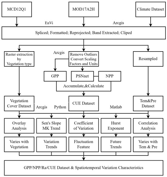
Figure 1.
The technical roadmap.
3. Results
3.1. Spatial Distribution Characteristics of CUE
Figure 2 illustrates the annual distribution of CUE in Southeastern Tibet, depicting the average total CUE from 2012 to 2022. The white regions depicted in the figure correspond to areas with missing data, signifying regions where data values are unavailable or undefined, characterized by a perennial absence of vegetation, water bodies, and snow-covered areas, where GPP and NPP values are consistently unavailable [41]. The average vegetation CUE in Southeastern Tibet exhibits fluctuations between 0 and 0.75, with a mean value of 0.67. Over 99% of the region demonstrates values between 0.64 and 0.75, indirectly indicating the precision of the data. The figure reveals an overall increasing trend in CUE from the central to the two sides, moving from south to north. These variations align with the spatial distribution patterns of elevation and land cover within the region.
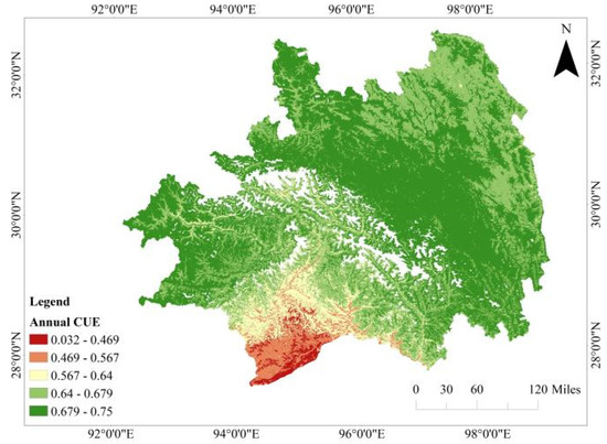
Figure 2.
The spatial distribution of the mean carbon use efficiency (CUE) in Southeastern Tibet from 2012 to 2022.
Specifically, regions with CUE levels between 0 and 0.4 cover 4.8% of the total area, predominantly concentrated in the southern evergreen broadleaf forests and evergreen coniferous forests. Sporadic occurrences extend towards the northern parts and partially transition east of Chamdo. Areas with CUE levels between 0.4 and 0.5 account for 1.47% of the total area, primarily distributed in the valleys below 2000 m in the southern region. This encompasses broadleaf forests, shrublands, sparse tree grasslands, and residential areas.
3.2. Seasonal and Interannual Variations in CUE
The temporal dynamics of CUE in Southeastern Tibet during representative months (a: January, b: April, c: July, d: October) over the years are depicted in Figure 3. The region exhibits a systematic cyclical variation in vegetation CUE throughout the year. From December to February, as shown in Figure 3a, the CUE in the Nyingchi area remains at a low level. During this winter period, a descending V-shaped demarcation line, centered around 29° N, segregates the region. In the northern part, CUE is characterized by no data, whereas in the southern part, CUE levels exceed 0.238, predominantly maintaining values above 0.468. Moving into March to May (Figure 3a,b), with rising temperatures and the onset of early vegetation growth, CUE exhibits a north-to-south ascending gradient in grasslands and coniferous forest regions, culminating at a specific threshold of 0.549. Simultaneously, CUE in the southern forested areas experiences a slight decrease of around 0.1 compared to the winter period. Transitioning from the early growth stage to the peak growth stage (Figure 3b,c), in fallow land, characterized by diminished vegetation cover, CUE experiences a swift ascent, surpassing 0.65. Similar elevations beyond 0.536 are observed in CUE for shrubland, coniferous forest, and mixed forest areas. Conversely, the CUE in evergreen broadleaf forest regions exhibits a persistent decline, reaching values at or below 0.5, with the southern border forest area exhibiting the lowest value in the region, dropping below 0.3 during this temporal interval. As the late growth stage ensues, excluding the southern evergreen broadleaf forest area, the majority of Nyingchi’s regions attain and stabilize within the elevated CUE zone, with mean CUE values exceeding 0.66. By October (Figure 3d), concurrent with declining temperatures and originating from the northern boundary, CUE undergoes a gradual reduction in shrubland, grassland, and fallow land, eventually reaching winter levels (below 0.3). Meanwhile, CUE in southern forested areas recommences an ascent, ultimately stabilizing at 0.65.
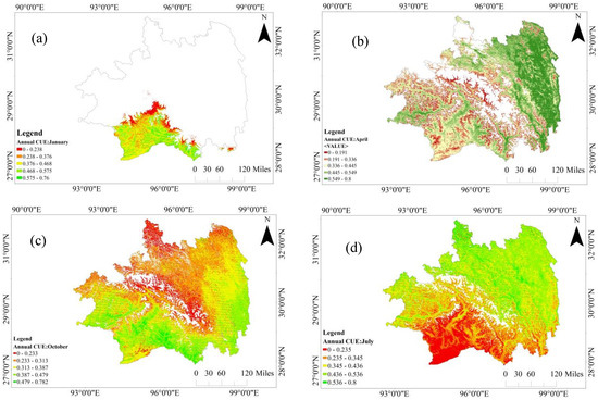
Figure 3.
The monthly variations in CUE from 2012 to 2022 during typical months. (a) January, (b) April, (c) July, (d) October.
Following the aforementioned exposition, the coefficient of variation (CV) is systematically derived for the monthly average CUE. This analytical procedure is implemented to precisely quantify the degree of variability and stability exhibited by vegetation throughout its growth cycle. The computed CV values are subsequently stratified into five distinct levels, adhering rigorously to the stipulated methodology. Illustrated in Figure 4, the region north of 28.5° N in Southeastern Tibet predominantly manifests low volatility in CUE. In the southern areas above an elevation of 1000 m, there is a discernible trend in evergreen broadleaf forest areas transitioning from high to relatively low volatility. As elevation and latitude increase, the vegetation types shift from broadleaf forests to coniferous forests, with a smaller proportion persisting as broadleaf forests, contributing to a gradual decline in CUE stability. The area north of 29° N, especially in the evergreen coniferous and mixed forest regions, emerges as the locale with the highest CUE stability, characterized by consistently low volatility over an extended temporal span.
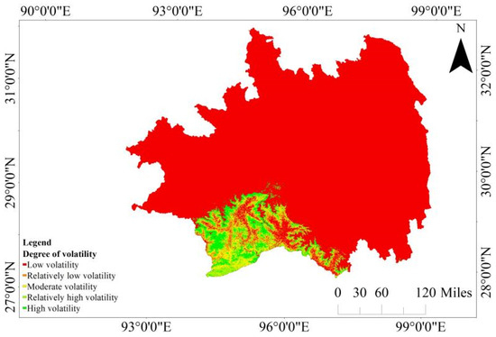
Figure 4.
The monthly CV of CUE in Southeastern Tibet. The CV values are computed to elucidate the degree of variability in CUE across different months, offering insights into the temporal dynamics and stability of vegetation in the region.
The line chart in Figure 4 illustrates the interannual variations in the average CUE over an 11-year period in Southeastern Tibet. The mean CUE within this geographical expanse consistently hovers around 0.66. An analysis employing a simple linear regression, wherein a trend line is fitted, reveals a gradual ascending trajectory in the annual average CUE for Southeastern Tibet. It is worth noting that the statistical significance of this observed trend is comparatively modest. As evident from Figure 4, the zenith of the annual mean CUE was observed in the year 2022, reaching a pinnacle of 0.676, whereas the nadir occurred in 2015, registering a minimum value of 0.665. The range of CUE fluctuations exceeds 0.01. Rapid declines in CUE were observed in 2014–2015 and 2019–2020, with a relatively stable increase from 2015 to 2017, recovering to a level of 0.661 in 2017. Subsequently, a sharp increase in CUE is observed after 2020. In summary, over the 11-year period, Southeastern Tibet exhibits an overall increasing trend in CUE.
Integrating the prevailing vegetation conditions, we have generated an interannual line graph depicting CUE variations across various vegetation types over the period spanning 2012 to 2022 (Figure 5). The graph elucidates distinct ranges and fluctuation patterns in CUE among diverse vegetation types. In open shrublands, the average CUE displays fluctuations ranging from 0.57 to 0.7, characterized by pronounced line undulations and a substantial overall range. Conversely, evergreen broadleaf forests and croplands interspersed with natural vegetation exhibit CUE averages ranging from 0.51 to 0.54 and 0.41 to 0.45, respectively, showcasing wider variability compared to other forest types. Mixed forests, closed shrublands, evergreen needleleaf forests, deciduous broadleaf forests, and deciduous needleleaf forests cluster within CUE values spanning 0.64 to 0.68, illustrating relatively stable levels with comparable overall fluctuation trends. Cultivated lands, urban areas, croplands, and grasslands maintain CUE averages within the range of 0.68 to 0.7, signifying elevated CUE values in the southeastern Tibetan Plateau. Within this set, barren lands, defined by vegetation cover less than 10%, showcase the highest levels of CUE. Notably, the interannual fluctuations in CUE for these four distinct land cover types are nominal, with annual averages indicating a state of relative constancy.
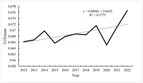
Figure 5.
Illustrates the interannual variations in the annual average CUE from 2012 to 2022.
3.3. Temporal and Spatial Trends in CUE
The continuous multi-year dataset of CUE was subjected to rigorous analysis using Sen’s slope estimation and MK trend analysis methodologies. The integration of these analytical approaches allowed for the categorization of trend characteristics into nine discrete classes. Figure 6 visually portrays both the distribution and proportional area of each identified trend class. Approximately 62.79% of the Southeastern Tibet region exhibits a declining trend in CUE. Within this category, 51.39% demonstrates a non-significant decrease, primarily distributed in the central Nyingchi area, encompassing broadleaf forests, needleleaf forests, mixed forests, and transitional zones between forests and grasslands. Areas characterized by a substantial or markedly substantial reduction in CUE account for 7.2% of the total region, predominantly concentrated in the southwestern sector of Nyingchi, proximate to the Himalayas. These areas include needleleaf forests and needleleaf–broadleaf mixed forests, as well as valley regions situated in the central and eastern sectors featuring mixed forests.
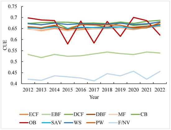
Figure 6.
The interannual CUE mean values for various vegetation types from 2012 to 2022 (ECF: Evergreen Coniferous Forest, EBF: Evergreen Broadleaf Forest, DCF: Deciduous Coniferous Forest, DBF: Deciduous Broadleaf Forest, MF: Mixed Forest, CB: Closed Bush, OB: Open Bush, SAV: Savannah, WS: Woody Savannah, PW: Permanent Wetland, F/NV: Farmland/Natural Vegetation Mosaic).
Conversely, a discernible ascending trend in CUE is observed in 36.95% of the Nyingchi region (Figure 7). Within this category, 33.02% exhibits a non-significant increase, predominantly in the northern part of Nyingchi, including Gungthang, Bomê County in the north, and grasslands in the central part of Zayü County in the south. Regions with a significant or highly significant increase constitute 2.33%, mainly found in the grasslands and barren lands of the Gangdise Range in southern Nyingchi, as well as the valley areas of the Yigong River and Neyang River upstream, characterized by a mixture of forests and grasslands.
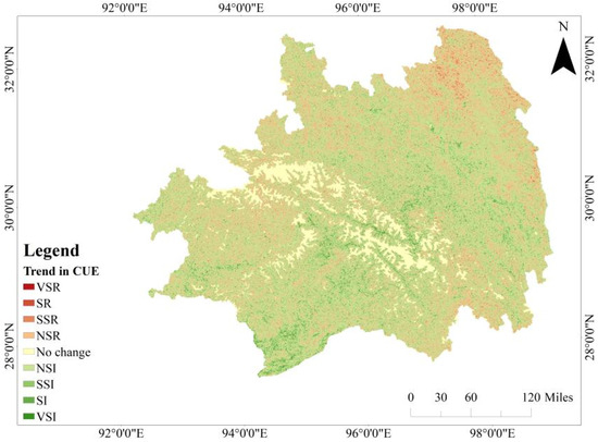
Figure 7.
Trends in CUE variation in Southeastern Tibet from 2012 to 2022 (VSI: very significant increase; SI: significant increase; SSI: slightly significant increase; NSI: no significant increase; NSR: no significant reduction; SSR: slightly significant reduction; SR: significant reduction; VSR: extremely significant reduction).
The outcomes derived from the application of the Hurst exponent method to scrutinize long-term persistent trends in CUE in Southeastern Tibet are presented in Figure 8. A substantial portion, approximately 75.95% of the region, displays a “counter-persistent” trend, suggesting that future variations are expected to oppose the current trends. In contrast, 24.05% of the region exhibits a “persistent” trend, indicating that future changes are likely to align with the existing trends. These areas are dispersed across various regions in Southeastern Tibet, with notable instances of robust “persistent” characteristics observed in the evergreen needleleaf forests in the southeast and west, as well as the evergreen broadleaf forests in southern Mêdog County.
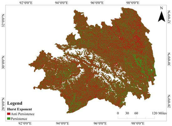
Figure 8.
Analysis results of the Hurst exponent for CUE in Southeastern Tibet.
The extrapolation of future trends in CUE in Southeast Tibet was achieved through the integration of long-term trends derived from the Hurst exponent analysis with Sen’s slope estimates and the outcomes of Mann–Kendall trend analysis. This amalgamation resulted in the production of a comprehensive map illustrating the anticipated trajectories of CUE over time in the specified region (Figure 8). Examining the figure reveals that 47.82% of the regions depict a transition from growth to decline in CUE, predominantly distributed in the grasslands northeast of Southeast Tibet and the central valleys on both sides of the Nyingchi region. Furthermore, a notable proportion of the regions, constituting 30.10%, exhibit a discernible reversal in trends, transitioning from a declining pattern to a growth-oriented trajectory. Predominantly situated in the northeastern grasslands and the southwestern evergreen coniferous forests, these areas showcase a pronounced shift in the observed temporal patterns. Regions with continuous CUE growth constitute 20.89%, scattered in the western grasslands, southern evergreen broadleaf forests, and the southeastern shrubland and sparsely wooded grassland. Areas where CUE is anticipated to decline occupy 1.19%, primarily distributed in the central region along the Yarlung Tsangpo River, the Himalayan mountainous region along the southwestern border, and near the Dambaqu and Changdu counties in the southeast.
3.4. Driving Factors of CUE
3.4.1. Correlation between CUE and Changes in Climate Factors
Based on the monthly dataset spanning 2012 to 2021, incorporating temperature, precipitation, and CUE, this study systematically explores the pixel-scale correlation between CUE and climatic factors. Analyzing the relationship at the pixel scale provides enhanced control over extraneous variables and mitigates the influence of extreme or abrupt fluctuations in temperature, precipitation, and CUE values.
Employing the previously stipulated partial correlation coefficient and associated significance test formula, this study systematically derives the partial correlation coefficient between CUE and temperature. This analytical process deliberately omits the influence attributable to precipitation, thereby enhancing precision in the examination of their interrelation. The outcomes, illustrated in Figure 9, reveal that the interval of the partial correlation coefficient between Southeast Tibet CUE and temperature is −0.09 to 0.13, indicative of a generally subdued correlation strength. Areas where a positive correlation is observed between CUE and temperature constitute 42.1% of the total spatial extent, particularly concentrated to the north of 27.5° N latitude. Notably, areas manifesting a robust positive correlation (r > 0.6) are predominantly distributed in the evergreen broadleaf forests of Motuo, the deciduous broadleaf forests of Milin and Langxian, mixed forests, and sparsely wooded grasslands in the northeast sector of Southeast Tibet. In contrast, areas demonstrating an inverse correlation between CUE and temperature constitute 57.9% of the entire geographical expanse. This concentration is notably observed to the south of 30.5° N latitude and to the north of 28.0° N latitude. Significant negative correlations (r < −0.6) are prevalent in areas such as the mixed forests, evergreen coniferous forests, and deciduous broadleaf forests to the west of Langxian and Gongbu Jiangda. Additionally, the southeast region of Southeast Tibet exhibits negative correlations in evergreen coniferous forests, grasslands, mixed shrublands, mixed forests, and deciduous broadleaf forests. Significance analysis results indicate that in 30.40% of Southeast Tibet, CUE demonstrates a noteworthy correlation with temperature (p < 0.05), while only 35.67% of regions exhibit an extremely non-significant correlation (p > 0.01). This non-significant correlation is primarily concentrated in the transitional zone with a coefficient of variation of |r| < 0.2 within the latitude range of 29° N to 30° N. In summary, the correlation between CUE and temperature in Southeast Tibet showcases a nuanced pattern: correlation strength and significance levels ascend gradually from the central region around 30.0° N latitude towards both the northern and southern extremes, with heightened correlations observed in valleys and vegetated regions.
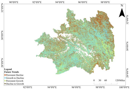
Figure 9.
The prospective evolution of CUE in Southeastern Tibet.
Subsequent to a methodologically rigorous approach, the study utilizes the designated partial correlation coefficient, along with its associated significance test formula. This analytical framework enables the precise computation of the partial correlation coefficient elucidating the nuanced relationship between CUE and precipitation, purposefully mitigating the confounding influence of temperature(Figure 10). As depicted in Figure 11, the partial correlation coefficient range characterizing the relationship between CUE and precipitation in Southeast Tibet exhibits fluctuations within the interval of −1.4 to 0.9. Notably, regions displaying a positive correlation between CUE and precipitation constitute 60.42% of the total geographical area, primarily concentrated between latitudes 28° N and 32.8° N, with smaller clusters in the central part of Southeast Tibet and north of Chamdo. Regions displaying high positive correlations (r > 0.3) are predominantly found in deciduous broadleaf forests and sparse tree grasslands at the southeastern boundary. Conversely, regions illustrating a negative correlation between CUE and precipitation cover 39.58% of the total area, with the majority distributed south of 28° N latitude and north of 30.5° N latitude. Areas with high negative correlations (r < −0.3) are mainly concentrated in the shrublands of Milin County.
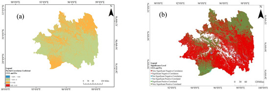
Figure 10.
The partial correlation coefficients (a) and the accompanying significance test results (b) for the relationship between CUE and precipitation in the Southeastern Tibet region.
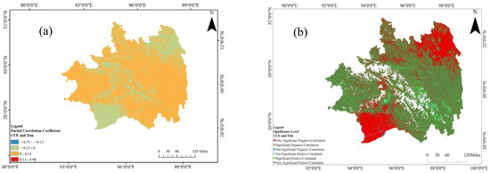
Figure 11.
The partial correlation coefficients (a) and the accompanying significance test results (b) for the relationship between CUE and temperature in the Southeast Tibet region.
In conjunction with the dual factors of precipitation and temperature overlaid in analysis (Figure 12), the correlation coefficient range between CUE and precipitation–temperature in the Southeast Tibet region spans from −1.22 to 0.81. Within this range, regions exhibiting a positive correlation between CUE and precipitation–temperature cover 74.52% of the total area. The predominant concentration of these positively correlated regions is observed between latitudes 28° N and 32° N, with minor distributions in the central to southern areas of Southeast Tibet and north of Chamdo. Areas with a heightened positive correlation (r > 0) are notably situated along the southeastern boundary in deciduous broadleaf forests and sparse grasslands, as well as in shrublands along the southwestern boundary. Conversely, regions where CUE demonstrates a negative correlation with precipitation and temperature are primarily located north of 28.0° N latitude and south of 31° N latitude. Those regions exhibiting a notably strong negative correlation (r < −0.74) are concentrated south of Motuo County in evergreen coniferous forests and north of Chamdo City in grasslands.
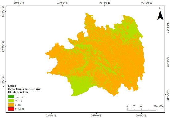
Figure 12.
The partial correlation coefficients between CUE and precipitation–temperature in the Southeast Tibet region.
Based on the aforementioned exposition, the impact of temperature and precipitation on CUE in the Southeast Tibet region reveals discernible trends, with temperature fluctuations exerting a more pronounced influence on CUE. Findings from a global-scale investigation conducted by Piao et al. point to a parabolic correlation between the annual average temperature and CUE in forest vegetation [31]. The extrapolation of this investigation to monthly intervals substantiates these findings. Additionally, within the southeastern Tibetan regions where the annual average temperature exceeds 12 °C or falls below 0 °C, heightened responsiveness of CUE to temperature is observed.
In contrast to temperature, the association between CUE and precipitation in Southeast Tibet appears to exhibit relatively diminished strength. Drawing from Zhang et al.’s expansive global-scale study on CUE, it is indicated that within the spectrum of annual precipitation below 2300 mm, there is an inverse relationship, such that the ratio of NPP to GPP diminishes with escalating precipitation levels. This assertion finds reinforcement in the northern sector of Nyingchi, particularly in areas where annual precipitation surpasses 700 mm. Nonetheless, in the central region of Southeast Tibet, characterized by an annual precipitation range spanning from 300 to 700 mm, an augmentation in precipitation levels corresponds to heightened values in both NPP and CUE. This observation suggests a plausible regional impact on CUE due to precipitation, particularly in the southern part of Nyingchi.
3.4.2. Changes in CUE in Response to Vegetation Growth Processes under Different Vegetation Types
Average data for NPP, GPP, Ra, and CUE during the growing season and the representations of diverse vegetation cover types in Southeast Tibet are delineated in Figure 11. Due to the combined influence of latitude and topography, the carbon sequestration process in areas with interspersed vegetation among shrublands and farmland (Figure 13a) exhibits the largest fluctuations, with the NPP/GPP/CUE amplitude in shrublands being the most significant. The CUE reaches its lowest value in February (below 0.2), suggesting reduced photosynthesis due to snow cover during this month. From February to June, CUE steadily increases, indicating a higher carbon fixation capacity during the spring growing season. Significant fluctuations in CUE are observed in July and October, with the lowest values, indicating that July and October, as typical growing periods, not only showcase strong carbon sequestration capabilities but also involve an increased release of carbon through respiratory consumption. Additionally, October records the lowest values for NPP/GPP/Ra.
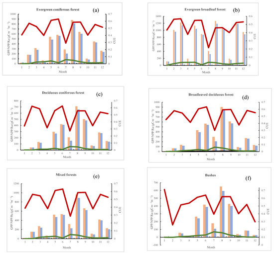
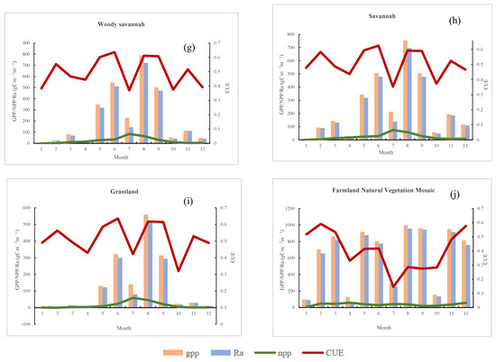
Figure 13.
The seasonal variation in mean GPP/NPP/Ra/CUE for various representative vegetation types. (a) Evergreen coniferous forest, (b) evergreen broadleaf forest, (c) deciduous coniferous forest, (d) broadleaved deciduous forest, (e) mixed forests, (f) bushes, (g) woody savannah, (h) savannah, (i) grassland, (j) farmland natural vegetation mosaic.
In areas with interspersed vegetation among farmland, CUE exhibits the most substantial fluctuation, declining continuously from January to the lowest value in July before slowly rising again until December. Minimal NPP/GPP/Ra values are observed in January and April, and this decline in January may be due to winter snow cover, resulting in a brief dormant period where vegetation does not photosynthesize. During this dormancy period, the NPP/GPP levels in vegetation among farmland are relatively low, causing CUE to drop to 0.4–0.5. In early April, during the initial growth phase, carbon fixation through photosynthesis is primarily used for the vegetation’s own growth, leading to a higher Ra. As seen in Figure 13j, NPP, GPP, and CUE exhibit similar high- and low-value periods in areas with interspersed vegetation among farmland, resembling the pattern observed in shrublands. A slight reduction in productivity is evident in June and July, with a peak in productivity occurring in August, suggesting that high summer temperatures may limit vegetation productivity.
CUE fluctuations in other vegetation types appear similar, with an increase in CUE observed after each growing season. Deciduous coniferous forests, deciduous broadleaf forests, and evergreen coniferous forests (depicted in Figure 13a,c,d) manifest notably congruent ranges and patterns in GPP, NPP, Ra, and CUE. The progression of GPP/NPP/Ra follows a seasonal pattern, with the highest values occurring in summer, succeeded by spring and autumn, and the lowest levels recorded in winter. The apex of CUE consistently transpires in April–May, coinciding with a rapid increase in GPP/NPP levels. This leads to the speculation that these three vegetation types exhibit elevated carbon sequestration levels in the initial growth stages, ensuring energy balance throughout their lifecycle.
The carbon sequestration process in evergreen broadleaf forests (Figure 13b) differs notably from other forest types. The pattern of GPP/NPP/CUE variations is characterized by high levels in autumn and spring and low levels in summer and winter, with minimal fluctuation (not exceeding 0.1). This observation implies a relatively consistent ratio of carbon consumption to production throughout the growth cycle. Among the various vegetation types, evergreen broadleaf forests manifest the highest GPP/NPP levels, concurrently exhibiting the greatest carbon release through respiration. In these forested ecosystems, the periods of elevated and reduced activity for GPP/NPP/CUE do not coincide, distinctly revealing a drop in productivity in June and July.
In grasslands and sparsely wooded grasslands (Figure 13e–g), productivity levels gradually decrease with decreasing vegetation coverage, especially in grasslands. NPP/GPP/Ra values are minimal from January to April and continue to decline after October. CUE exhibits larger fluctuations, with peak periods occurring in the vigorous growth season from June to August. In contrast to regions characterized by abundant vegetation coverage, areas with sparse vegetation exhibit a discernible delay in the occurrence of peak CUE periods. GPP/NPP/Ra/CUE in grasslands and sparsely vegetated wooded grasslands indirectly highlight the heightened sensitivity of plant productivity in low vegetation coverage areas to temperature and precipitation.
4. Discussion
This investigation delineates the temporal dynamics of CUE in vegetation across the Southeastern Tibetan Plateau from 2012 to 2022, shedding light on critical interplays with climatic variables and vegetation characteristics. Notably, the overarching trend reveals a fluctuating increase in vegetation CUE during the specified timeframe, punctuated by discernible downturns in 2015 and 2022. These inflections correlate precisely with interannual variations in temperature and precipitation, encapsulating a period marked by decreasing precipitation and escalating temperatures in the region, thereby substantiating the empirical evidence of a warming trend in Southeastern Tibet. At a monthly temporal scale, the observed ascent in CUE from the early to late growing season, progressing from the southern to northern reaches of the Southeastern Tibetan Plateau, parallels findings by Zhang et al., affirming a substantive correlation between vegetation CUE and temperature and precipitation dynamics [36]. Simultaneously, regions characterized by heightened CUE values exhibit lower coefficients of variation, denoting a more stabilized state in CUE dynamics. The preponderance of grassland as the dominant vegetation type in most areas adds a crucial layer to the complexity of these dynamics [42,43,44,45].
This study underscores the divergent sensitivities of forest and farmland CUE to precipitation in contrast to the susceptibility of grassland and shrubland CUE to temperature fluctuations. These disparities emanate from inherent dissimilarities in the biological and ecological profiles of distinct biotic communities. In synthesizing these analyses, it becomes evident that the variability in vegetation CUE is intricately intertwined with both climatic influences and the inherent distribution and biological attributes of specific vegetation types. The dataset reveals that grassland and sparse grassland consistently manifest higher annual CUE values relative to woody plant counterparts. As illustrated in Figure 5, the annual CUE in these low-vegetation regions stabilizes at around 0.65 over the eleven-year period. The concomitant elevation in CUE stability correlates with diminishing vegetation cover (grassland > sparse grassland > shrubland > forest). Drawing from extant research, the conjecture posits three primary factors contributing to the elevated CUE in regions with low vegetation cover. Firstly, within non-woody vegetation types prevalent in the four delineated ecological systems, the widespread distribution of herbaceous plants, mosses, and lichens emerges. Their lack of stems, branches, and leaves translates to diminished water resistance and augmented photosynthetic rates [35,37]. A plethora of studies affirm the general proclivity of herbaceous plants and mosses towards higher CUE compared to alternative vegetation types. Moreover, cultivated crops exhibit a proclivity for elevated CUE in comparison to their natural counterparts. Secondly, attention is drawn to the constraints inherent in large-scale vegetation remote sensing, notably through MODIS. The granularity of MOD17A2 (500 m) in capturing vegetation productivity proves limited, particularly in areas of low vegetation cover where NPP/GPP falls below 5 gC·m−2 [37]. This study aligns with existing literature suggesting that MODIS CUE tends to skew higher than values derived from empirical measurements, especially in regions characterized by low biomass, where MODIS NPP and GPP fall below literature-derived benchmarks [35,45,46,47]. Evidently, reliance on conventional large-scale vegetation remote sensing methodologies over the preceding three decades proves less precise [48]. The burgeoning prominence of advanced vegetation sensing technologies, specifically Sun-Induced Chlorophyll Fluorescence (SIF), emerges as a promising paradigm to mitigate the limitations inherent in traditional vegetation remote sensing. The existing spectrum signals emitted from plant-based photosynthetic centers (650–800 nanometers), featuring two peaks in red light (around 690 nanometers) and near-infrared light (around 740 nanometers), serve as indicators of the dynamic changes in actual photosynthesis and vegetation growth status. This information is employed for the exploration of vegetation productivity, offering novel perspectives and technologies for land carbon cycling and remote sensing vegetation monitoring [49,50]. Research conducted by Qiu et al. suggests that the capability of GOSIF (Gross Primary Productivity Solar-Induced Fluorescence) in estimating GPP exceeds that of MODIS GPP products. With the advancement of high-resolution spectral sensors deployed on satellites, analogous satellite-derived SIF products are anticipated to demonstrate substantial potential in the future. This not only paves the way for enhanced precision in discerning potential photosynthetic mechanisms but also augments the toolkit available for land ecosystem carbon cycling investigations and advanced vegetation monitoring [51,52,53].
In Section 3.2, as depicted in Figure 5, it is discernible that the CUE within the southeastern Tibetan Plateau (CUE-TP) consistently maintains an average value of approximately 0.67. Nevertheless, recent years have witnessed pronounced fluctuations in CUE, hinting at an augmented prospective variability in CUE dynamics, thereby elucidating the precarious stability of carbon sequestration in the high-altitude forest ecosystem of Southeastern Tibet. The MOD12Q1 dataset illuminates a discernible reduction in vegetation coverage in this region over the preceding years, concomitant with a proportional escalation in bare land and snow/ice coverage [53,54]. The conspicuous degradation of vegetation in the southeastern Tibetan Plateau, attributed to global climate warming and modest anthropogenic activities, has precipitated significant ramifications such as the deterioration of vegetation and heightened soil erosion [55]. Consequently, these phenomena detrimentally influence plant growth, thereby intensifying the fluctuations in NPP, GPP, and CUE within the region.
Hence, ecological conservation emerges as an exigent priority. The primary imperative lies in the preservation and elevation of forest productivity. Strategies encompass the curtailment of illicit logging, safeguarding pristine forests, orchestrating the rehabilitation of forest productivity, instating artificial afforestation endeavors, and expanding forested areas. Simultaneously, addressing and managing grassland degradation through judicious pastoral practices is crucial. This includes the prevention of soil erosion and desertification, the preservation of ecological equilibrium, and the concomitant enhancement of carbon sequestration and storage efficiency within forest ecosystems. These measures collectively contribute to the advancement of ecosystem sustainability [55].
5. Conclusions
Grounded in MODIS GPP and PSNnet data, this study endeavors to discern the spatiotemporal characteristics and driving factors of CUE in the pristine forests of Southeastern Tibet from 2012 to 2022. The following conclusions are drawn:
- Temporal Dynamics at Monthly and Annual Scales:
At the monthly scale, the regional CUE exhibits notable variations throughout the growing season, with distinct patterns across different vegetation types. High-altitude forested areas display minimal intra-annual CUE fluctuations, while evergreen needleleaf and broadleaf forests exhibit more pronounced variations. On an annual scale, the overall trend indicates a non-significant upward trajectory in CUE, yet a notable intensification in CUE variability is observed during the period from 2019 to 2022.
- 2.
- Climate-Driven CUE Variability in Southeastern Tibet:
CUE in Southeastern Tibet displays sensitivity to temperature and precipitation changes, with temperature exerting a more significant influence, particularly evident in the pronounced correlations observed in Gongjue County and Changdu Town. Intriguingly, temperature and precipitation exhibit inverse impacts on the CUE trend in the region. The geographic location and climatic conditions of vegetation contribute to the variations observed. Vegetation located at 28.5° N in the southern and northern regions of Southeastern Tibet responds differently to temperature and precipitation changes, with temperature alterations demonstrating a more pronounced impact. Vegetation in areas characterized by unique topography exhibits heightened sensitivity to climate variations.
- 3.
- Vegetation Type as a Predominant Determinant of CUE Variation:
The type of vegetation emerges as the primary factor shaping the range and features of CUE variation. Grassland and sparse grassland regions consistently manifest notably higher CUE values compared to evergreen broadleaf forests, deciduous broadleaf forests, evergreen needleleaf forests, and deciduous needleleaf forests. Additionally, areas where shrubland intermingles with farmland vegetation exhibit significantly higher CUE variability compared to other vegetation types within the study sites.
In summation, this research underscores the intricate interplay between climatic factors, geographical attributes, and vegetation types in influencing the spatiotemporal dynamics of CUE in Southeastern Tibet. The insights garnered contribute to a more nuanced understanding of the intricate ecological processes governing carbon utilization efficiency in this ecologically vital region.
Author Contributions
Q.S.: Conceptualization, Methodology, Software, Investigation, Data Processing, Data Curation, Analysis, Writing—Original Draft; J.L. (Corresponding Author): Conceptualization, Resources, Software, Investigation, Data Processing, Validation, Arrangement, Writing—Review and Editing; Q.Y.: Conceptualization, Funding Acquisition, Resources, Supervision, Writing—Review and Editing; J.H.: Resources, Software, Investigation, Data Processing, Validation, Arrangement, Writing—Review and Editing. All authors have read and agreed to the published version of the manuscript.
Funding
Key Open Topic of the Ministry of Education Key Laboratory for Forest Ecology in the Tibetan Plateau: “Temporal and Spatial Characteristics of Carbon Utilization Efficiency in Representative Forest Ecosystems of Southeastern Tibet and Influencing Factors” (XZA-JYBSYS-2023-04).
Data Availability Statement
The MODIS and meteorological data utilized in this study are publicly available in public repositories. MOD17A2H (GF) and MCD12Q1 can be accessed from NASA MODIS Web (http://modis.gsfc.nasa.gov/, accessed on 12 October 2023). Monthly average temperature and precipitation data can be obtained from the National Tibetan Plateau Science Data Center (https://data.tpdc.ac.cn/, accessed on 30 October 2023).
Acknowledgments
We would like to thank NASA for providing the MODIS Gross and Net Primary Productivity (MOD17A2H) and the Land Cover Monitoring Productivity (MCD12Q1) data (http://modis.gsfc.nasa.gov/, accessed on 12 October 2023). We also acknowledge the National Tibetan Plateau Science Data Center for providing temperature and precipitation data (https://data.tpdc.ac.cn/, accessed on 30 October 2023). We would also like to acknowledge the valuable suggestions from the anonymous reviewers of this manuscript.
Conflicts of Interest
The authors declare no conflicts of interest.
References
- Heimann, M.; Reichstein, M. Terrestrial ecosystem carbon dynamics and climate feedbacks. Nature 2008, 451, 289–292. [Google Scholar] [CrossRef]
- Schimel, D.; Pavlick, R.; Fisher, J.B.; Asner, G.P.; Saatchi, S.; Townsend, P.; Miller, C.; Frankenberg, C.; Hibbard, K.; Cox, P. Observing terrestrial ecosystems and the carbon cycle from space. Global Change Biol. 2015, 21, 1762–1776. [Google Scholar] [CrossRef]
- Li, B.; Huang, F.; Qin, L.; Qi, H.; Sun, N. Spatio-Temporal Variations of Carbon Use Efficiency in Natural Terrestrial Ecosystems and the Relationship with Climatic Factors in the Songnen Plain, China. Remote Sens. 2019, 11, 2513. [Google Scholar] [CrossRef]
- Guenther, A. The contribution of reactive carbon emissions from vegetation to the carbon balance of terrestrial ecosystems. Chemosphere 2002, 49, 837–844. [Google Scholar] [CrossRef]
- Hou, H.; Zhang, S.; Ding, Z.; Huang, A.; Tian, Y. Spatiotemporal dynamics of carbon storage in terrestrial ecosystem vegetation in the Xuzhou coal mining area. China Environ. Earth Sci. 2015, 74, 1657–1669. [Google Scholar] [CrossRef]
- Chen, J.M.; Ju, W.; Ciais, P.; Viovy, N.; Liu, R.; Liu, Y.; Lu, X. Vegetation structural change since 1981 significantly enhanced the terrestrial carbon sink. Nat. Commun. 2019, 10, 4259. [Google Scholar] [CrossRef] [PubMed]
- Fatichi, S.; Pappas, C.; Zscheischler, J.; Leuzinger, S. Modelling carbon sources and sinks in terrestrial vegetation. New Phytol 2018. [Google Scholar] [CrossRef]
- Miller, S.D.; Goulden, M.L.; Menton, M.C.; Da, R.; Humberto, R.; De, F.; Helber, C.; Figueira, A.; Michela, S.; Dias, S.; et al. Biometric and micrometeorological measurements of tropical forest carbon balance. Ecol. Appl. 2004, 14, 114–126. [Google Scholar] [CrossRef]
- Fang, J.; Guo, Z.; Shilong, P.; Chen, A. Terrestrial vegetation carbon sinks in China 1981–2000. Sci. China Ser. D 2007, 50, 1341–1350. [Google Scholar] [CrossRef]
- Gao, H.; Dong, L.; Li, F.; Zhang, L. Evaluation of Four Methods for Predicting Carbon Stocks of Korean Pine Plantations in Heilongjiang Province, China. PLoS ONE 2015, 10, e0145017. [Google Scholar] [CrossRef]
- Zeng, W.S. Development of monitoring and assessment of forest biomass and carbon storage in China. For. Ecosyst. 2014, 1, 20. [Google Scholar] [CrossRef]
- Strohbach, M.W.; Arnold, E.; Haase, D. The carbon footprint of urban green space-A life cycle approach. Landsc. Urban. Plan. 2012, 104, 220–229. [Google Scholar] [CrossRef]
- Pan, Y.; Birdsey, R.A.; Fang, J.; Houghton, R.; Kauppi, P.E.; Kurz, W.A.; Phillips, O.L.; Shvidenko, A.; Lewis, S.L.; Canadell, J.G.; et al. A Large and Persistent Carbon Sink in the World’s Forests. Science 2011, 333, 988–993. [Google Scholar] [CrossRef]
- Fang, J.Y.; Liu, G.H.; Xu, S.L. Biomass and net production of forest vegetation in China. Acta Ecol. Sin. 1996, 16, 497–508. [Google Scholar]
- Wu, S.; Li, J.; Zhou, W.; Lewis, B.J.; Yu, D.; Zhou, L.; Jiang, L.; Dai, L. A statistical analysis of spatiotemporal variations and determinant factors of forest carbon storage under China’s Natural Forest Protection Program. J. For. Res. 2018, 29, 415–424. [Google Scholar] [CrossRef]
- Piao, S.L.; Fang, J.Y.; Zhou, L.M.; Zhu, B.; Tan, K.; Tao, S. Changes in vegetation net primary productivity from 1982 to 1999 in China. Glob. Biogeochem. Cycles 2005, 19. [Google Scholar] [CrossRef]
- Gao, Y.; Zhou, X.; Wang, Q.; Wang, C.; Zhan, Z.; Chen, L.; Yan, J.; Qu, R. Vegetation net primary productivity and its response to climate change during 2001–2008 in the Tibetan Plateau. Sci. Total Environ. 2013, 444, 356–362. [Google Scholar] [CrossRef]
- Wu, Y.Y.; Wu, Z.F. Quantitative assessment of human-induced impacts based on net primary productivity in Guangzhou, China. Environ. Sci. Pollut. Res. 2018, 435, 11384–11399. [Google Scholar] [CrossRef]
- Gitelson, A.A.; Vina, A.; Masek, J.G.; Verma, S.B.; Suyker, A.E. Synoptic monitoring of gross primary productivity of maize using Landsat data. IEEE Geosci. Remote Sens. Lett. 2008, 5, 133–137. [Google Scholar] [CrossRef]
- Peng, Y.; Gitelson, A.A.; Sakamoto, T. Remote estimation of gross primary productivity in crops using MODIS 250 m data. Remote Sens. Environ. 2013, 128, 186–196. [Google Scholar] [CrossRef]
- Zhu, W.Z. Advances in the carbon use efficiency of forest. Chin. J. Plant Ecol. 2013, 37, 1043–1058. [Google Scholar] [CrossRef]
- An, X.; Chen, Y.; Tang, Y. Factors affecting the spatial variation of carbon use efficiency and carbon fluxes in east Asia forest and grassland. Res. Soil. Water Conserv. 2017, 24, 79–92. [Google Scholar]
- El, M.B.; Schwalm, C.; Huntzinger, D.N. Carbon and Water Use Efficiencies: A Comparative Analysis of Ten Terrestrial Ecosystem Models under Changing Climate. Sci. Rep. 2019, 9, 14680. [Google Scholar]
- Collalti, A.; Trotta, C.; Keenan, T.F. Thinning Can Reduce Losses in Carbon Use Efficiency and Carbon Stocks in Managed Forests Under Warmer Climate. J. Adv. Model. Earth Syst. 2018, 10, 2427–2452. [Google Scholar] [CrossRef]
- DeLucia, E.H.; Drake, J.E.; Thomas, R.B. Forest carbon use efficiency: Is respiration a constant fraction of gross primary production. Glob. Chang. Biol. 2007, 13, 1157–1167. [Google Scholar] [CrossRef]
- He, Y.; Piao, S.; Li, X.; Chen, A.; Qin, D. Global patterns of vegetation carbon use efficiency and their climate drivers deduced from MODIS satellite data and process-based models. Agric. For. Meteorol. 2018, 256, 150–158. [Google Scholar] [CrossRef]
- Li, B.; Huang, F.; Chang, S. The Variations of Satellite-Based Ecosystem Water Use and Carbon Use Efficiency and Their Linkages with Climate and Human Drivers in the Songnen Plain, China. Adv. Meteorol. 2019, 2019, 1–15. [Google Scholar] [CrossRef]
- Ye, X.; Liu, F.; Zhang, Z.; Xu, C.; Liu, J. Spatio-temporal variations of vegetation carbon use efficiency and potential driving meteorological factors in the Yangtze River Basin. J. Mt. Sci. 2020, 17, 1959–1973. [Google Scholar] [CrossRef]
- Luo, X.; Jia, B.; Lai, X. Quantitative analysis of the contributions of land use change and CO2 fertilization to carbon use efficiency on the Tibetan Plateau. Sci. Total Environ. 2020, 728, 138607. [Google Scholar] [CrossRef]
- Liu, J.; Deng, X.; Hou, M.; Wang, X.; Shi, Z.; Ni, S. Thermodynamic control on chemical weathering of river bedrock at the Aba and Qamdo in Kaschin-beck disease region, eastern Tibet Plateau. Geosystems Geoenviron. 2022, 100126. [Google Scholar] [CrossRef]
- Yang, L.; Shen, F.X.; Zhang, L.; Cai, Y.Y.; Yi, F.X.; Zhou, C.H. Quantifying influences of natural and anthropogenic factors on vegetation changes using structural equation modeling: A case study in Jiangsu Province, China. J. Clean. Prod. 2021, 280, 124330. [Google Scholar] [CrossRef]
- Yan, L.; Zhou, G.S.; Wang, Y.H.; Hu, T.Y.; Sui, X.H. The spatial and temporal dynamics of carbon budget in the alpine grasslands on the Qinghai-Tibetan Plateau using the Terrestrial Ecosystem Model. J.Clean. Prod. 2015, 107, 195–201. [Google Scholar] [CrossRef]
- Xiong, H.B.; Shi, H.Y.; Xiao, Z.Q. Consistent retrieval of multiple parameters from GOES-R top of atmosphere reflectance data. Int. J. Remote Sens. 2020, 41, 7931–7957. [Google Scholar] [CrossRef]
- Wang, Y.; Wei, J.; Zhou, J.; Yang, J.; Xu, Y.; Chen, Y.; Hao, J.; Cheng, W. Ecological Sensitivity Assessment of the Southeastern Qinghai-Tibet Plateau using GIS and AHP—A Case Study of the Nyingchi Region. J. Resour. Ecol. 2023, 14, 158–166. [Google Scholar]
- Du, L.; Gong, F.; Zeng, Y.; Ma, L.; Qiao, C.; Wu, H. Carbon use efficiency of terrestrial ecosystems in desert/grassland biome transition zone: A case in Ningxia province, northwest China. Ecol. Indic. 2021, 120, 106971. [Google Scholar] [CrossRef]
- Running, S.W.; Zhao, M. Daily GPP and annual NPP (MOD17A2/A3) products NASA Earth Observing System MODIS land algorithm. MOD17 User’s Guide 2015, 2015, 1–28. [Google Scholar]
- Zhao, Y.L.; Liu, H.X.; Zhang, A.B.; Cui, X.M.; Zhao, A.Z. Spatiotemporal variations and its influencing factors of grassland net primary productivity in Inner Mongolia, China during the period 2000–2014. J. Arid Environ. 2019, 165, 106–118. [Google Scholar] [CrossRef]
- Sun, G.; Liu, X.; Wang, X.; Li, S. Changes in vegetation coverage and its influencing factors across the Yellow River Basin during 2001–2020. J. Desert Res. 2021, 41, 205. [Google Scholar]
- Zhang, Y.; Hu, Q.W.; Zou, F.L. Spatio-Temporal Changes of Vegetation Net Primary Productivity and Its Driving Factors on the Qinghai-Tibetan Plateau from 2001 to 2017. Remote Sens. 2021, 13, 1566. [Google Scholar] [CrossRef]
- Yang, Z.Y.; Yu, Q.; Yang, Z.Y.; Peng, A.C.; Zeng, Y.F.; Liu, W.; Zhao, J.K.; Yang, D. Spatio-Temporal Dynamic Characteristics of Carbon Use Efficiency in a Virgin Forest Area of Southeast Tibet. Remote Sens. 2023, 15, 2382. [Google Scholar] [CrossRef]
- Jin, Y.; Lu, H.F.; Guo, X.L.; Gong, X. Multiscale Analysis of Flow Patterns in the Dense-Phase Pneumatic Conveying of Pulverized Coal. AIChE J. 2019, 65, e16674. [Google Scholar] [CrossRef]
- Sang, W.G.; Chen, S.; Li, G.Q. Dynamics of leaf area index and canopy openness of three forest types in a warm temperate zone. J. Plant Ecol. 2008, 3, 416–421. [Google Scholar] [CrossRef]
- Piao, S.; Luyssaert, S.; Ciais, P.; Janssens, I.A.; Chen, A.; Cao, C.; Fang, J.; Friedlingstein, P.; Luo, Y.; Wang, S. Forest annual carbon cost: A global-scale analysis of autotrophic respiretion. Ecology 2010, 91, 652–661. [Google Scholar] [CrossRef]
- Yu, G.; Ren, W.; Chen, Z.; Zhang, L.; Wang, Q.; Wen, X.; He, N.; Zhang, L.; Fang, H.; Zhu, X.; et al. Construction and progress of Chinese terrestrial ecosystem carbon, nitrogen and water fluxes coordinated observation. J. Geogr. Sci. 2016, 26, 803–826. [Google Scholar] [CrossRef]
- Amthor, J.S. The McCree–de Wit–Penning de Vries–Thornley respiration paradigms: 30 years later. Ann. Bot. 2000, 86, 1–20. [Google Scholar] [CrossRef]
- Street, L.E.; Subke, J.A.; Sommerkorn, M.; Sloan, V.; Ducrotoy, H.; Phoenix, G.K.; Williams, M. The role of mosses in carbon uptake and partitioning in arctic vegetation. New Phytol. 2013, 199, 163–175. [Google Scholar] [CrossRef]
- Amthor, J.S. Respiration and Crop Productivity; Springer Science & Business Media: New York, NY, USA, 2012. [Google Scholar]
- Zhang, Y.; Xu, M.; Chen, H.; Adams, J. Global pattern of NPP to GPP ratio derived from MODIS data: Effects of ecosystem type, geographical location and climate. Glob. Ecol. Biogeogr. 2009, 18, 280–290. [Google Scholar] [CrossRef]
- Huang, X.; Xiao, J.; Wang, X.; Ma, M. Improving the global MODIS GPP model by optimizing parameters with FLUXNET data. Agric. For. Meteorol. 2021, 300, 108314. [Google Scholar] [CrossRef]
- Chen, J.; Zhang, H.; Liu, Z.; Che, M.; Chen, B. Evaluating parameter adjustment in the MODIS gross primary production algorithm based on eddy covariance tower measurements. Remote Sens. 2014, 6, 3321–3348. [Google Scholar] [CrossRef]
- Lin, X.; Chen, B.; Chen, J.; Zhang, H.; Sun, S.; Xu, G.; Guo, L.; Ge, M.; Qu, J.; Li, L.; et al. Seasonal fluctuations of photosynthetic parameters for light use efficiency models and the impacts on gross primary production estimation. Agric. For. Meteorol. 2017, 236, 22–35. [Google Scholar] [CrossRef]
- Dong, H.; Guo, H.; Yuan, Y. Estimation of Terrestrial Ecosystem GPP Based on Sun-induced Chlorophyll Fluorescence. Trans. Chin. Soc. Agric. Mach. 2019, 50, 205–211.64. [Google Scholar]
- Liu, X.; Liu, Z.; Liu, L.; Lu, X.; Chen, J.; Du, S.; Zou, C. Modelling the influence of incident radiation on the SIF-based GPP estimation for maize. Agric. For. Meteorol. 2021, 307, 108522. [Google Scholar] [CrossRef]
- Sun, Z.; Gao, X.; Du, S.; Liu, X. Research Progress and Prospective of Global Satellite-based Solar-induced Chlorophyll Fluorescence Products. Remote Sens. Technol. Appl. 2021, 36, 1044–1056. [Google Scholar]
- Qiu, R.; Han, G.; Ma, X.; Xu, H.; Shi, T.; Zhang, M. A comparison of OCO-2 SIF, MODIS GPP, and GOSIF data from gross primary production (GPP) estimation and seasonal cycles in North America. Remote Sens. 2020, 12, 258. [Google Scholar] [CrossRef]
Disclaimer/Publisher’s Note: The statements, opinions and data contained in all publications are solely those of the individual author(s) and contributor(s) and not of MDPI and/or the editor(s). MDPI and/or the editor(s) disclaim responsibility for any injury to people or property resulting from any ideas, methods, instructions or products referred to in the content. |
© 2024 by the authors. Licensee MDPI, Basel, Switzerland. This article is an open access article distributed under the terms and conditions of the Creative Commons Attribution (CC BY) license (https://creativecommons.org/licenses/by/4.0/).