Response of Vegetation Productivity to Greening and Drought in the Loess Plateau Based on VIs and SIF

Abstract

In the context of global warming, the frequent occurrence of drought has become one of the main reasons affecting the loss of gross primary productivity (GPP) of terrestrial ecosystems. Under the influence of human activities, the vegetation greening trend of the Loess Plateau increased significantly. Therefore, it is of great significance to study the response of GPP to drought in the Loess Plateau under the greening trend. Here, we comprehensively assessed the ability of vegetation indices (VIs) and solar-induced chlorophyll fluorescence (SIF) to capture GPP changes at different seasonal scales and during drought. Specifically, we utilized three vegetation indices: normalized difference vegetation index (NDVI), near-infrared reflectance of vegetation (NIR_V), and kernel NDVI index (kNDVI), and determined the drought period of the Loess Plateau in 2001 based on the standardized precipitation evapotranspiration index (SPEI) and the standardized soil moisture index (SSMI). Moreover, the anomalies of VIs and SIF during the drought period and the relationship with GPP anomalies were compared. The results showed that both SIF and VIs were able to capture changes during the drought period as well as in normal years. Overall, SIF captured drought changes better due to water and heat stress as well as GPP changes compared to VIs. Across different time scales, SIF showed the strongest relationship with GPP (meanR² = 0.85), followed by NIR_V (meanR² = 0.84), NDVI (meanR² = 0.76), and kNDVI (meanR² = 0.74), suggesting that SIF is more sensitive to physiological changes in vegetation. Notably, kNDVI performed best in sparse vegetation (meanR² = 0.85). In capture during drought, NIR_V and kNDVI performed better in less productive land classes; SIF showed superior capture as land use class productivity increased. In addition, GPP anomalies correlated better with kNDVI anomalies (meanR² = 0.50) than with other index anomalies. In the future, efforts to integrate the respective strengths of SIF, NIR_V, and kNDVI will improve our understanding of GPP changes.

1. Introduction

Gross primary productivity (GPP) is the amount of organic carbon fixed by plants via photosynthesis per unit time [1], and is the largest and most uncertain component of the global carbon cycle [2]. As the basis of human production and life, changes in GPP are related to human welfare. Understanding how photosynthesis responds to global environmental change is particularly important because small perturbations in terrestrial productivity have implications for global biodiversity, agriculture, and climate change [3,4].

Long-term satellite data show a significant greening trend in global vegetation area since the 1980s, driven by human land use management (e.g., revegetation in China), climate change, and CO₂ fertilization [5,6]. Continued greening has led to an increase in vegetation productivity. According to recent studies, the global terrestrial carbon sink increased from (−0.2 ± 0.9) Pg C yr⁻¹ (1 Pg = 10¹⁵ g) in the 1960s to (1.9 ± 1.1) Pg C yr⁻¹ in the 21st decade [7]. Changes in evapotranspiration (ET) due to vegetation greening can also have an impact on local/regional climate. In general, an increase in ET due to the greening of vegetation enhances the local water vapor cycle, leading to an increase in precipitation in downwind areas and a weak but significant downward trend in near-surface air temperatures [8]. There is increasing evidence that the greater atmospheric water demand with rising temperatures (i.e., radiative effects of CO₂) may lead to an increased intensity and frequency of drought, which could notably affect vegetation growth and crop yields [9,10,11]. Drought is a persistent and abnormal shortage of rainfall. The World Meteorological Organization (WMO) classified drought according to the affected domain as meteorological, agricultural, hydrological, and socioeconomic [12]. Drought is one of the most prevalent natural disasters in the world and has the most severe and widespread impacts on terrestrial ecosystem GPP. Droughts have tremendous impacts on ecosystem composition, structure, and functioning, largely affecting GPP accumulation and weakening the carbon sink function of terrestrial ecosystems [13,14,15]. In addition to this, drought events are often associated with complex emergencies involving multiple and compound hazards (e.g., food shortages, economic crises, or human/livestock/crop diseases). The interaction between a number of such factors can affect exposure, vulnerability, and capacity to cope with the crisis. Therefore, it is important to study the response of GPP to drought under the greening trend for future agricultural security and ecological protection.

Changes in gross primary productivity (GPP) profoundly affect food security and the stability of the carbon cycle. Among the methods of ground-based observation of GPP, the inventory method estimates changes in carbon stocks in terrestrial ecosystems based on comparisons of inventory data from different periods. The lack of long-term continuous inventory data and the uncertainty of the conversion process from sample points to regional scales have led to a large bias in the results at the regional scales [16]. The eddy covariance (EC) technique is considered to be the most stable and accurate method for estimating GPP at the ecosystem scale [17]. It is based on the principle of micrometeorology and directly measures the net CO₂ exchange between land ecosystems and the atmosphere over a fixed coverage area. Nevertheless, the number of EC stations is sparse and unevenly distributed, making it challenging to study aspects of GPP at the regional scale [18]. The remote sensing technique is more effective than the ground-based observation method. Remote sensing techniques are well suited to monitor changes in ecosystem GPP at broad spatial scales compared to ground-based observation methods. Over the past 40 years, a series of time-continuous and spatially consistent GPP products have been generated based on satellite remote sensing, providing directly observed data for ecosystem research and management [19]. Thus, in this paper, Moderate-resolution Imaging Spectroradiometer (MODIS) GPP products were used to analyze the study area.

Vegetation indices (VIs) based on remotely sensed reflectance, which have been widely used to monitor changes in vegetation growth, can help us to better understand the changes in GPP in areas during periods of drought [20]. Previous studies have shown that the normalized difference vegetation index (NDVI) can indicate the greenness of vegetation and can be used to monitor vegetation growth [21]. Two recently developed indices, near-infrared reflectance of vegetation (NIR_V) and kernel NDVI (kNDVI), both of which solve the background contamination problem well, are stronger than NDVI in linking with GPP [22,23]. NIR_V only needs to input two parameters when estimating GPP, which drastically reduces the complexity of GPP estimation. It has been shown that NIR_V can replace SIF to study the photosynthesis of vegetation [24]. The coupling between the components of canopy structure that influence NIR reflectance and stress-constrained canopy photosynthetic capacity remains strong at drought stress events, making NIR_V and GPP maintain a strong coupling during drought events [24]. kNDVI computes all higher-order relationships for NDVI and resolves the nonlinear relationship with GPP. kNDVI is more highly correlated with GPP and less problematic in terms of noise and instability than products such as NDVI and NIR_V [23].

Solar-induced chlorophyll fluorescence (SIF) is a promising index for satellite monitoring of vegetative photosynthesis. It is fundamentally different from VIs. SIF is a product of vegetative photosynthesis, which can reflect the intensity of vegetative photosynthesis and has a very close physiological and metabolic connection with GPP [25,26,27,28,29,30]. It is well known that an arid environment will weaken the photosynthesis ability and metabolic function of plants, which in turn will weaken the signal release of SIF. VIs are only sensitive to changes in the canopy structure and chlorophyll concentration of vegetation and are not directly related to the photosynthesis of plants. Hence, when drought occurs, the greenness of vegetation does not decrease immediately, resulting in a certain lag effect of vegetation indexes on drought [31,32,33]. Compared with VIs, SIF has a more sensitive response to drought and is more suitable for monitoring changes in GPP during drought.

China has one of the widest distribution of ecologically fragile areas in the world, accounting for 22% of the national territory, with diverse types of fragility and severe vulnerability [34]. The Loess Plateau in China has experienced severe vegetation loss, soil erosion, and land degradation [35]. In view of this, China has carried out a series of ecological restoration measures, the most successful of which was the Grain for Green Project in 1999 [36]. This project aims to prevent soil erosion, alleviate flooding, and store carbon by increasing forest and grassland cover on previously cropped hillslopes, as well as converting cropland, barren hills, and wasteland into forested areas [37]. Using the ecological restoration measures, the Loess Plateau has shown a clear trend of “greening” [38,39,40]. However, the region is still vulnerable to disturbance and damage, and ecological restoration is difficult, with low carrying capacity, which is an obstacle to carbon reduction and sequestration. Drought will make the fragile ecosystem of the Loess Plateau more unstable and cause irreversible impacts on the ecosystem. The rising greening trend and unstable climate change in the Loess Plateau bring great challenges to GPP’s accounting. Therefore, it is important to study the response of GPP to drought under the greening trend of the Loess Plateau.

In this paper, the Loess Plateau was selected as the study area, and land cover types were reclassified. The spatial and temporal characteristics of GPP, drought, and greening of different land cover types on the Loess Plateau were investigated, as well as the relationship between GPP and VIs and SIF in different time scales and drought periods, which are of great significance for the sustainable development of the Loess Plateau. The objectives of this paper are: (1) to analyze the drought changes in the Loess Plateau from 2001 to 2020 and identify drought events; (2) to analyze the spatial and temporal changes of VIs (NDVI, NIR_V, and kNDVI), SIF and GPP from 2001 to 2020, and identify the trends of the greening and the GPP; (3) analyze the correlations of VIs and SIF with GPP at different time scales; (4) to reveal the performance of VIs and SIF in capturing GPP changes under drought events. For (3) and (4), we hypothesize that SIFs perform better than VIs based on previous studies. The main contribution of this paper is to analyze the relationship between VIs and SIF with GPP at different time scales in terms of different land types on the Loess Plateau, as well as compare the ability of the two to capture GPP changes during drought.

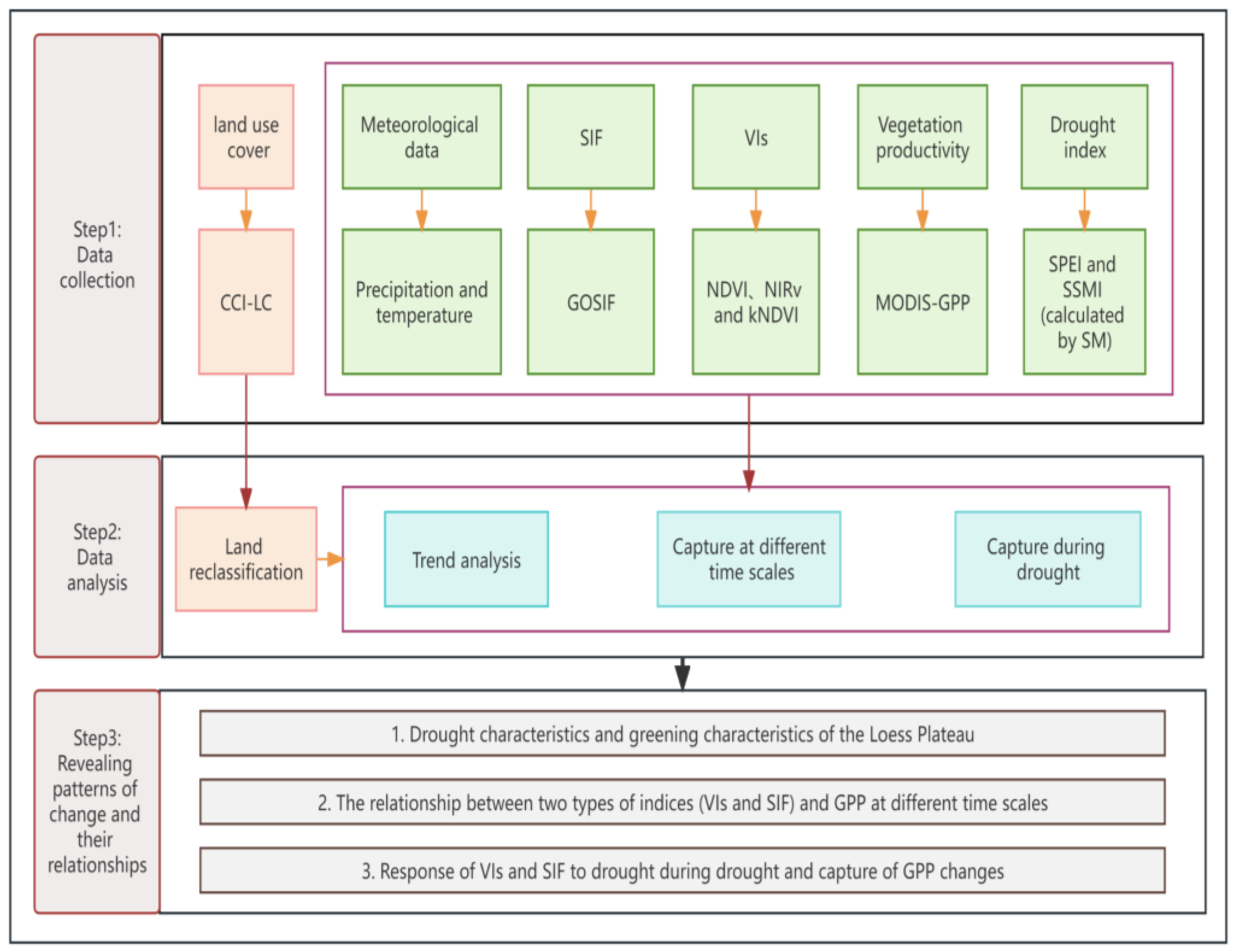
2. Materials and Methods

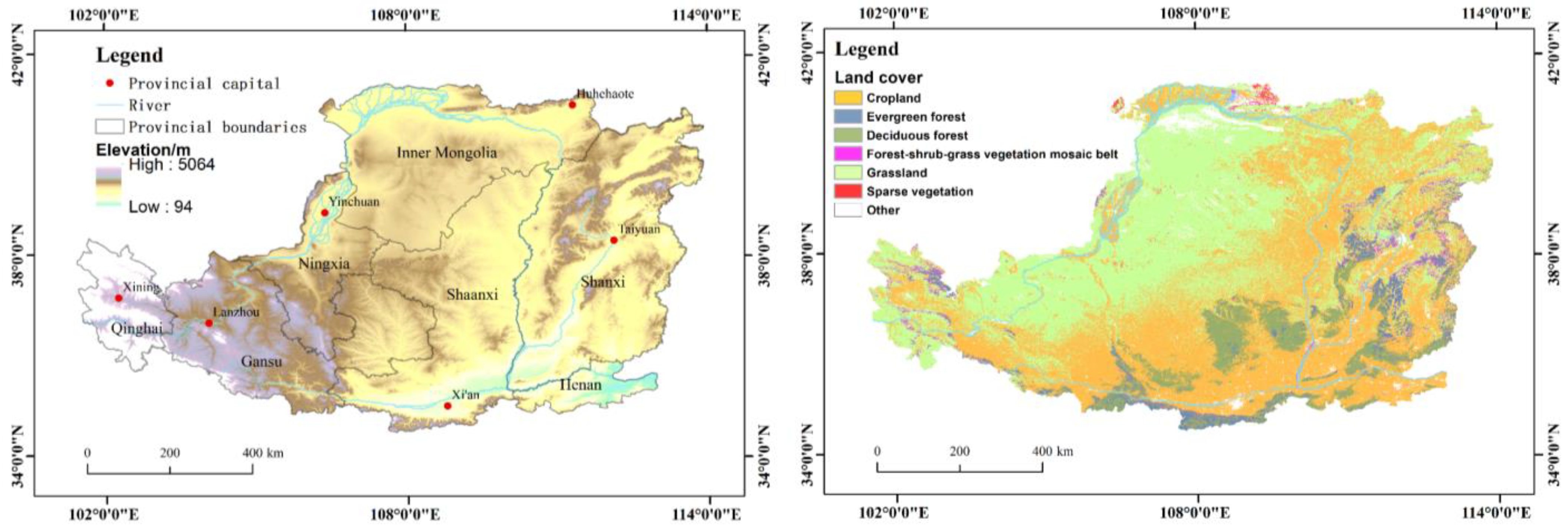
Taking drought stress caused by climate change and vegetation greening caused by human action as perspectives, drought indices (SPEI and SSMI) and MODIS products were selected to analyze the spatial and temporal characteristics of drought, GPP, and greening as well as the relationships among them in the study area. Specifically, this paper first analyzed the spatial and temporal characteristics of drought, GPP, and greening under different land cover types in the Loess Plateau from 2001 to 2020. Secondly, the relationships between VIs and SIF with GPP at different time scales, such as spring, summer, autumn, and growing seasons, were analyzed. Finally, the performance of VIs and SIF in capturing GPP changes under drought periods was compared based on the differential changes of VIs, SIF, and GPP during drought, and the correlation of GPP anomalies with VIs and SIF anomalies was analyzed (Figure 1).

2.1. Study Area

The Loess Plateau is located in the north-central part of China, between 100°54′–114°33′ E and 33°43′–41°16′ N, with an east–west length of about 1300 km, a north–south width of about 800 km, and a total area of roughly 6.4 × 10⁵ km² [41]. The average annual temperature ranges from 3.6 °C to 14.3 °C, decreasing from southeast to northwest; the annual precipitation ranges from 150 mm to 750 mm, decreasing from southeast to northwest; the average annual evaporation ranges from 1400 mm to 2000 mm, decreasing from northwest to southeast, and the overall dryness is relatively high. Precipitation is concentrated in summer and autumn, winter and spring drought and little rain; the terrain is high in the west and low in the east, belonging to the typical semi-arid continental monsoon climate [42]. The ecology of the Loess Plateau has been very fragile for a long time due to intense human activities. In order to improve the regional environment, since 1999, the Loess Plateau has implemented a large-scale Grain for Green Project, and vegetation and ecology have been significantly restored [43]. However, the region is still sensitive to climate change, and frequent droughts seriously jeopardize regional environmental security and agricultural production. Most of the Loess Plateau is in semi-arid areas, and water availability is a major limiting factor for vegetation health and growth [35]. The planting of large-scale plantation forests in recent years may exacerbate water scarcity [44].

In this paper, we reclassify the land use types of the Loess Plateau using the annual global land cover dataset (Climate change initiative-landcover, CCI-LC). We categorized the land use cover types of the Loess Plateau into sparse vegetation, grassland, cropland, forest-shrub-grass vegetation mosaic belt, deciduous forest, evergreen forest, and others [45], of which sparse vegetation, grassland, cropland, forest-shrub-grass vegetation mosaic belt, deciduous forest, and evergreen forest accounted for 0.3%, 41.4%, 41.3%, 2.0%, 7.8%, and 3.0% of the Loess Plateau, respectively (Figure 2).

2.2. Data

2.2.1. Solar-Induced Chlorophyll Fluorescence (SIF) Data

In this paper, a global dataset of solar-induced chlorophyll fluorescence (GOSIF) data were utilized for the study. The GOSIF dataset was developed by Li and Xiao (2019) (https://globalecology.unh.edu/data.html, accessed on 30 October 2023) [28]. It is based on discrete SIF data from the Orbiting Carbon Observatory-2 (OCO-2SIF), MODIS data, and meteorological data and are obtained using machine learning methods [30]. The dataset has a high spatial and temporal resolution (0.05°, 8 days) and a correlation of 0.73 with the data from 91 global flux sites. Monthly scale data from 2001–2020 have been used in this paper.

2.2.2. MODIS Product Data

The vegetation indices used in this paper are NDVI, NIR_V, and kNDVI. We obtained MODIS-derived NDVI (MCD43A4_006_NDVI) from Google Earth Engine for the years 2001 to 2020. In addition, the computed NIR_V and kNDVI were calculated for MCD43A4 Nadir BRDF-Adjusted Reflectance Daily 500 m product hosted on Google Earth Engine. The NIR_V computation consists of two steps, first obtaining the median values of the red (620–670 nm) and NIR (841–876 nm) bands for each image-month scale in the study area and then calculating the NDVI from Equation (1), the NIR_V was calculated from Equation (2). Before calculating the NIR_V, 0.08 was subtracted from all NDVI values to account for the NDVI of partially bare soil. kNDVI was calculated from Equation (3).

$$NDVI=\frac{NIR-Red}{NIR+Red}$$

(1)

$${NIR}_V=(NDVI-0.08)\times NIR$$

(2)

$$kNDVI=tanh({(\frac{NIR-Red}{2\sigma })}^2)$$

(3)

where σ is an adjustable length scale parameter, here set to 0.5 (NIR + Red), thus simplifying the equation to kNDVI = tanh((NDVI)²).

GPP was obtained via Google Earth Engine using a 500 m resolution, 8-day cumulative synthetic product (MOD17A2H). In order to be consistent with the spatial and temporal resolution of the acquired SIF data, we computed all of GPP, NDVI, NIR_V, and kNDVI as monthly scale data and resampled to 0.05°.

2.2.3. Drought Index and Meteorological Data

The Standardized Precipitation Evapotranspiration Index (SPEI) was first proposed by Vicent Serrano et al. in 2010 [46], which in turn takes into account the evapotranspiration demand (potential evapotranspiration) compared to the Standardized Precipitation Index (SPI) and is able to better respond to different drought types and their impacts in the context of global warming. In this paper, a high-resolution SPEI dataset (SPEI_RF) is used, with highly consistent spatial and temporal distribution characteristics with the currently widely recognized SPEIbase v. 2.6 (developed by Vicente Serrano) dataset. Compared to the SPEIbase v. 2.6 dataset, the SPEI_RF dataset has the advantage of higher spatial resolution and more accurate identification of localized small-scale droughts [47].

The drought index is a convenient tool for assessing drought, and relying on meteorological factors to assess drought allows for long-term analysis but ignores the influence of surface factors on drought [48]. It is increasingly recognized that more diverse representations of water demand and supply by different land surface processes should be used to assess the extent of drought [49,50]. Accordingly, in this paper, we add soil moisture (SM) data and transform it into a standardized soil moisture index (SSMI), which, together with SPEI, indicates drought [51]. We use the Global 1 km resolution surface soil moisture dataset (2000–2020) [52]. This dataset is based on the secondary development of ESA-CCI active-passive fusion product, which integrates the ERA5 reanalysis data and utilizes multi-source remote sensing data to construct a machine learning algorithm to generate a global spatio-temporal continuous 1 km resolution surface soil moisture dataset for the years 2000–2020. Validated by 2346 ground observation stations worldwide, the results show that the product has good accuracy (correlation coefficient is 0.89, and the unbiased root mean square error is 0.045 m³/m³). SSMI calculation formula:

$$SSMI=\frac{SM-\overline{SM}}{SM\sigma }$$

(4)

where SM is the value of soil moisture at moment t, $\overline{SM}$ is the mean value of soil moisture from 2001 to 2020, and SMσ is the standard deviation of SM from 2001 to 2020. SPEI and SSMI drought classifications are shown in

Table 1. SPEI and SSMI drought classification.

SPEI	SSMI	Class
>−0.5	>0	No drought
−1.0–−0.5	−1.0–0	Mild drought
−1.5–−1.0	−1.5–−1	Moderate drought
−2.0–−1.5	−2.0–−1.5	Severe drought
≤−2	≤−2	Extreme drought

(SPEI is classified according to fB/T 24081-2017 of China Meteorological Administration [53], and SSMI is classified according to Zhou et al. [51]). To be consistent with the SIF data, the SPEI data and SM data were resampled at 0.05°.

In addition to this, precipitation (UCSB-CHG/CHIRPS/DAILY) and temperature (ECMWF/ERA5/DAILY) data were obtained from Google Earth Engine, and both were converted to monthly scale data.

2.3. Methodology

2.3.1. Trend Analysis and Significance Tests

To analyze the interannual spatial and temporal trends of drought, greening, and GPP, we used the Theil-Sen Median trend analysis and the Mann–Kendall (M-K) trend test. Where SPEI was calculated using SPEI_12 for December. SSMI was calculated by synthesizing the monthly scale SM data into annual-scale SM data according to the method of averaging before performing the trend calculation and then calculating it as SSMI by using the formula. The combination of Sen trend analysis and M-K test has been applied in many studies and is a well-established method in time series analysis. Sen trend analysis is a very robust nonparametric trend calculation method, compared with ordinary linear regression analysis, is insensitive to measurement error and outlier data and can reduce the impact of outliers [54,55]. The M-K test is a non-parametric statistical test based on rank [56]. It does not require the data to conform to a particular distributional state and is not affected by outliers.

2.3.2. Correlation of GPP with VIs and SIF

To monitor vegetation productivity, we analyzed the correlation of GPP with VIs and SIF at different time scales. Pearson correlation utilizes statistical theories and methods to quantify the degree of correlation between two variables and has been widely used in ecological and earth science research [57]. Here, we used the coefficient of determination (square of the correlation coefficient, R²) to quantify the correlation.

We combine SPEI_01 and SSMI, both of which reach the drought level at the same time (SPEI ≤ −0.5, SSMI ≤ 0) and last for three months to be considered as a drought event (the year in which it occurs is a drought year) [58]. To analyze the ability of VIs and SIF to capture GPP losses during a drought event, we compared the changes in SIF, VIs, and GPP, expressed as the ratio of the difference (drought year-reference year) to the reference year (average value from 2001 to 2020). Finally, the standardized anomalies of VIs and SIF during drought events in the Loess Plateau were calculated, and the correlation analysis of GPP anomalies with VIs and SIF anomalies was done. The anomaly calculation was similar to the SSMI formula, and the anomalies were categorized into five classes (

Table 2. Classes of anomalies.

Anomaly	Class
>2	Strong positive anomaly
1–2	Moderate positive anomaly
−1–1	No anomaly
−1–−2	Moderate negative anomaly
<−2	Strong negative anomaly

) [59].

3. Results

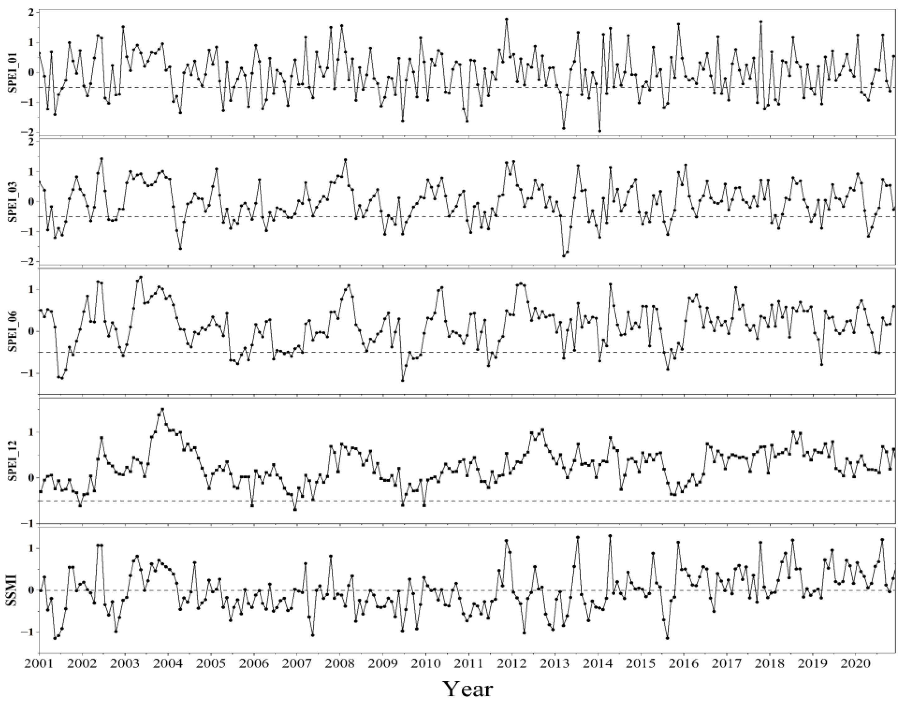
3.1. Drought Characteristics of the Loess Plateau

3.1.1. Spatial and Temporal Variability of Drought

Spatial and temporal variations of SPEI and SSMI from 2001 to 2020 were analyzed to determine the interannual wet and dry conditions on the Loess Plateau. The monthly, seasonal, semi-annual, and annual trends of SPEI are presented in Figure 3. SPEI fluctuates greatly on short time scales (monthly and seasonal scales) and then slows down with increasing time scales. SPEI_01 has the most frequent wet and dry variations, with a total of 62 drought months occurring from 2001 to 2020, of which there were 39 months of mild droughts, 19 months of moderate droughts, and 4 months of severe droughts, with no extreme droughts. The longest drought period was from May to July 2001. Compared with the monthly scale, the seasonal scale of SPEI_03 shows relatively stable wet and dry changes, with a total of 52 drought months, 41 of which were mild droughts, 8 were moderate droughts, 3 were severe droughts, and there were no extreme droughts. The longest drought period was from May to August 2001. SPEI_06 was significantly slower than the previous two short time scales, with a total of 29 drought months, 26 of which were mild droughts, 3 were moderate droughts, and no severe or extreme droughts. SPEI_12 was the most stable, with only 5 mild drought months. SM data were used and converted to SSMI to reflect the wet and dry status of the soil. During the period 2001–2020, 133 drought months were identified, accounting for more than half of the entire study period, and were dominated by mild drought, with 128 months of mild drought, 5 months of moderate drought, and no severe or extreme drought.

The spatial trends of SPEI and SSMI were analyzed using Sen trend analysis and the M-K test (Figure 4a,b). SPEI showed an increasing trend in all land cover types. However, the percentage of areas with significant increase was small, with sparse vegetation, grassland, cropland, forest-shrub-grass vegetation mosaic belt, deciduous forest, and evergreen forest with significant increase accounting for 2.01%, 7.19%, 6.87%, 3.01%, 3.74%, and 3.56% of their respective areas, respectively. The SSMI was in an upward trend in sparse vegetation, grassland, cropland, forest-shrub-grass vegetation mosaic belt, and in a downward trend in deciduous and evergreen forests. Among them, grassland and cropland had the most significant increase, accounting for 54.97% and 43.11% of their respective regions, while cropland, deciduous forest, and evergreen forest had significant decreases, accounting for 11.37%, 58.33%, and 20.34% of their respective regions, and in particular, the area with highly significant decreases in deciduous forest reached 34.24%. From the viewpoint of the entire Loess Plateau, the trend of drought is decreasing, and drought has weakened.

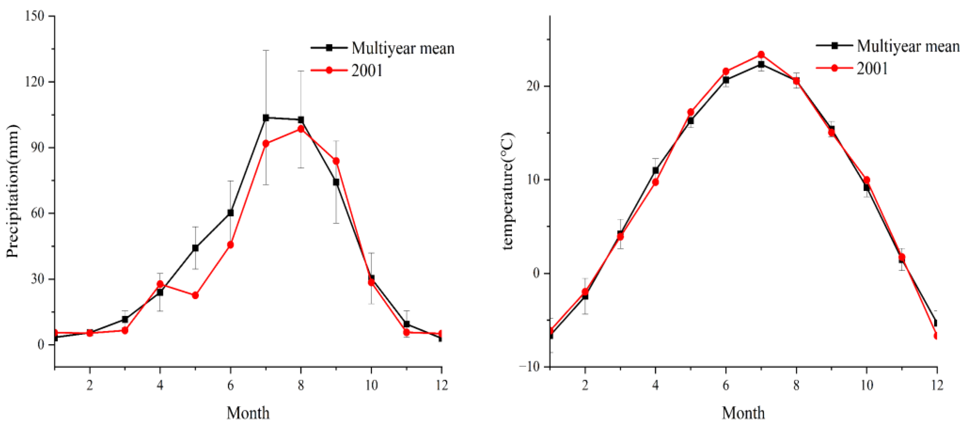
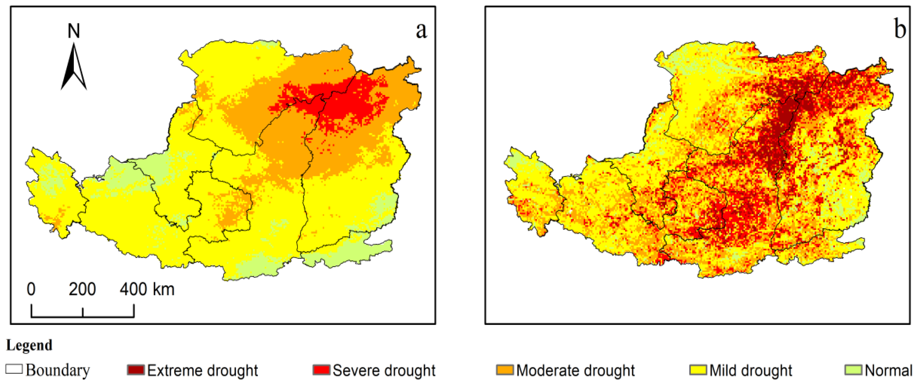
3.1.2. Characteristics of the 2001 Drought

As shown in Figure 5, precipitation dropped sharply in March and May 2001 and did not reach a return to normal levels until September. The average temperature for the May–July period was also higher than the multi-year average. The values of the SPEI for May–July were −1.407, −0.742, and −0.534, respectively, and the values of the SSMI were −1.149, −1.083, and −0.915, reaching almost all three months the moderate drought level. Therefore, May–July 2001 was identified as the drought event studied in this paper, and 2001 was designated as a drought year.

Figure 6 shows the spatial distribution of SPEI_01 and SSMI during the 2001 drought in the Loess Plateau. The study area suffered from low precipitation and high temperatures from May to July 2001, resulting in a basic drought condition in the region. The SPEI shows that 6.14% of the area was in severe drought, 26.15% in moderate drought, and 57.30% in mild drought. The severe drought region is mainly concentrated in the junction of Inner Mongolia, Shaanxi, and Shanxi, which is an interlace zone of grassland and cropland. The moderate drought area is an extension of the severe drought area, occupying the northeastern part of the study area as well as part of the central part. The western and southern parts of the study area are relatively less arid. The SSMI shows a higher degree of aridity, with 8.54% extreme drought, 15.90% severe drought, 29.72% moderate drought, and 39.61% mild drought. The areas of extreme drought continue to be concentrated near the junction of Inner Mongolia, Shaanxi, and Shanxi. Severe and moderate droughts are widely distributed in each province. The spatial drought characteristics of SPEI and SSMI are similar, but the drought degree of SSMI is more severe. This should make us realize the importance of combining meteorological drought with land surface drought processes.

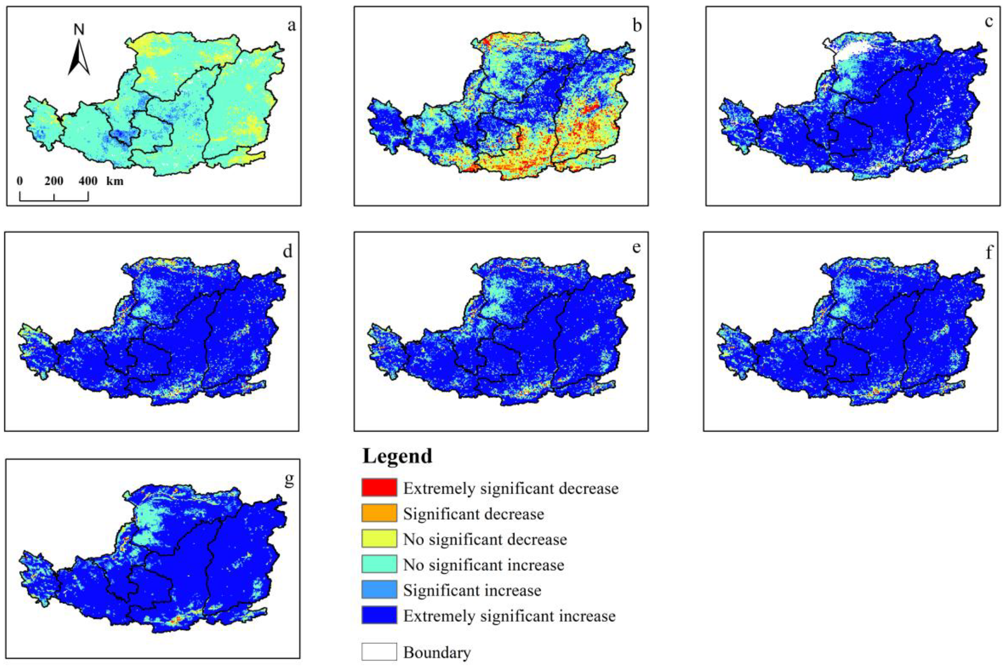
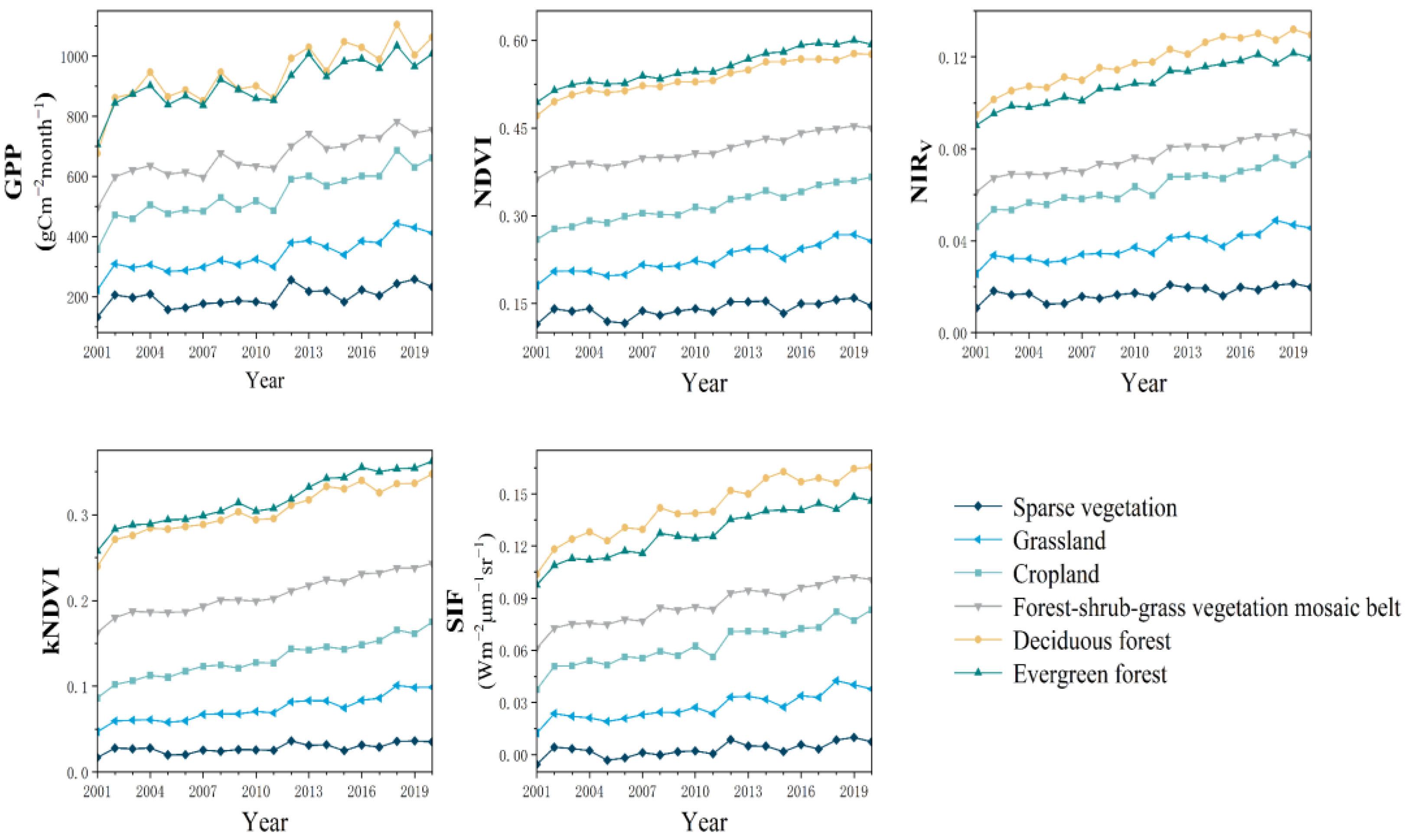
3.2. Greening Characteristics of the Loess Plateau

Each index showed an increasing trend in all land cover types (Figure 7), indicating that the Grain for Green Project played a significant role in greening the vegetation and sequestering carbon in the Loess Plateau. However, only SIF and NIR_V reflected the phenomenon that the GPP of deciduous forests was higher than that of evergreen forests. The spatial trends of VIs, SIF, and GPP were analyzed using Sen trend estimation and M-K test (Figure 4c–g). VIs, SIF, and GPP showed stable significant and highly significant increasing trends in most regions. This coincided with the temporal trends of annual-scale VIs and SIF (Figure 7). In western Inner Mongolia and northern Ningxia VIs, SIF and GPP showed insignificant increasing trends. Each index of forest land in Shaanxi and Shanxi showed a certain downward trend, which corresponded to the trend of SSMI forest land. In addition to cropland (which is supposed to be the reason for artificial intervention), the proportion of very significant increase areas increased with the increase in the productivity of land types (from low to high: sparse vegetation, grassland, forest-shrub-grass vegetation mosaic belt, and forest land).

3.3. Relationship of GPP with VIs and SIF, 2001–2020

To analyze the correlation of GPP with VIs and SIF during the study period, we performed correlation analyses for spring, summer, autumn, non-growing season, growing season, removal of winter (removing the value of winter), and the entire study period (all months) from 2001 to 2020 (Figure 8). Looking at the different time scales, the correlation in the non-growing season was relatively low compared to the other time scales, which may be due to the weak photosynthesis in the non-growing season when the vegetation grows slowly or does not grow. In both deciduous and evergreen forests, summer correlations were also much lower compared to other seasonal scales.

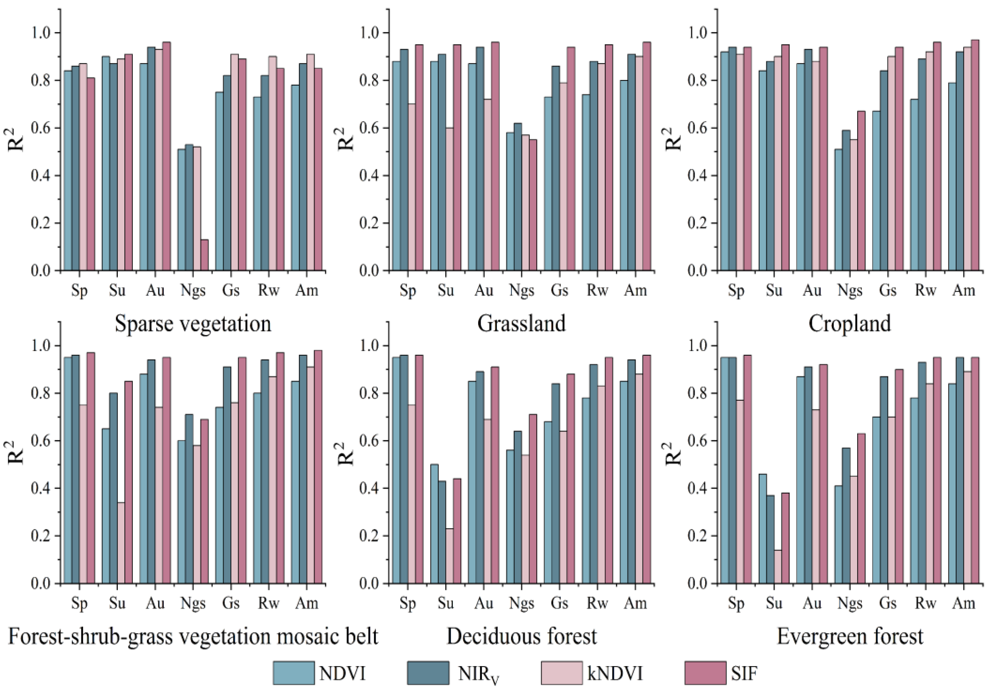
3.3.1. Correlation of GPP with VIs

The kNDVI-GPP relationship (meanR² = 0.74) was the lowest among the three VIs. Specifically, the kNDVI-GPP relationship was significantly lower in grassland, forest-shrub-grass vegetation mosaic belt, deciduous forest, and evergreen forest than in NDVI and NIR_V. Compared to sparse vegetation and cropland, the kNDVI-GPP relationship for grassland, forest-shrub-grass vegetation mosaic belt, deciduous forest, and evergreen forest declined the most in spring, summer, and autumn. In particular, the R² of kNDVI-GPP for forest-shrub-grass vegetation mosaic belt, deciduous forest, and evergreen forest in summer was only 0.34, 0.23, and 0.14. It is noteworthy that kNDVI performed best in sparse vegetation (meanR² = 0.85). Although the NDVI-GPP relationship was lowest during the growing season, removal of winter, and entire study period (excluding the growing season in deciduous forests) in each of the land classes, the NDVI-GPP relationship (meanR² = 0.76) remained slightly higher than kNDVI.

The NIR_V-GPP relationship (meanR² = 0.84) was much improved across vegetation types compared to NDVI and kNDVI. The correlation with GPP was much higher than that of NDVI and kNDVI in all land types except in sparse vegetation and cropland, where it was slightly lower than kNDVI. NIR_V performed best in the non-growing season (meanR² = 0.61) and even outperformed SIF in sparse vegetation, grassland, and forest-shrub-grass vegetation mosaic belt.

3.3.2. Correlation between GPP and SIF

The SIF-GPP relationship (meanR² = 0.85) improved compared to VIs. Moreover, SIF performs worse than VIs in some land classes and on certain time scales, which denied the original hypothesis that SIF performed best. Specifically, in sparse vegetation, it was lower than at least one of the indices in the VIs at other time scales except summer and autumn and was especially lowest in the non-growing season (R² = 0.13). In addition, it was lower than NIR_V in the non-growing season in grassland and forest-shrub-grass vegetation mosaic belts and lower than NDVI in summer in deciduous and evergreen forests.

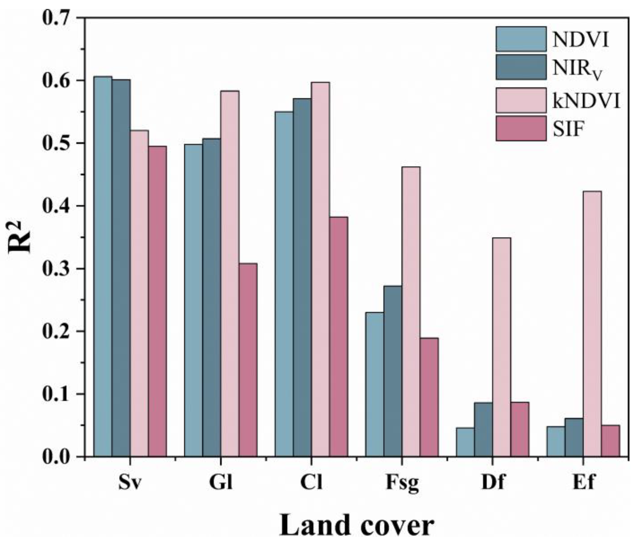
3.4. Capture of GPP by VIs and SIF in Dry Years

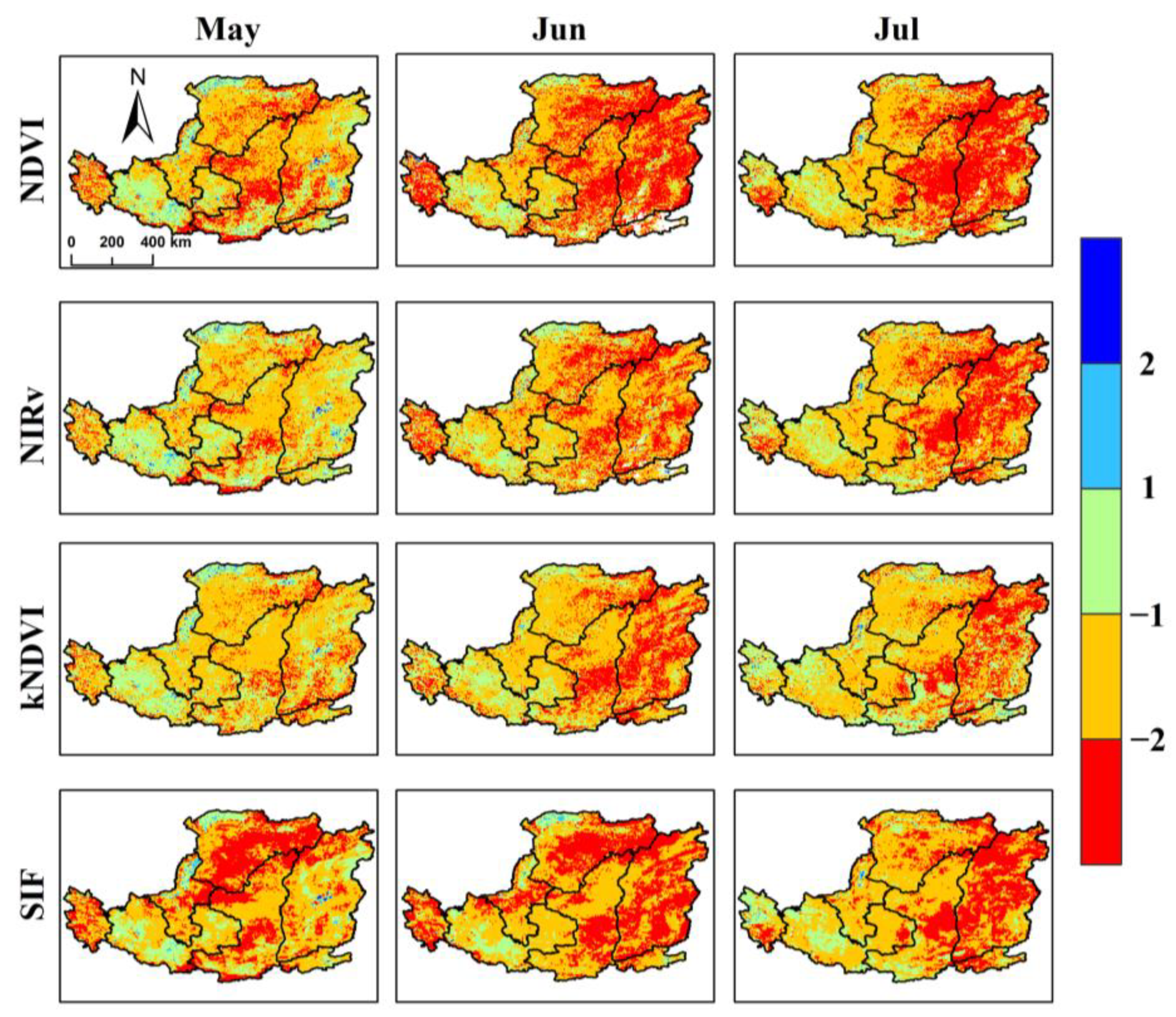
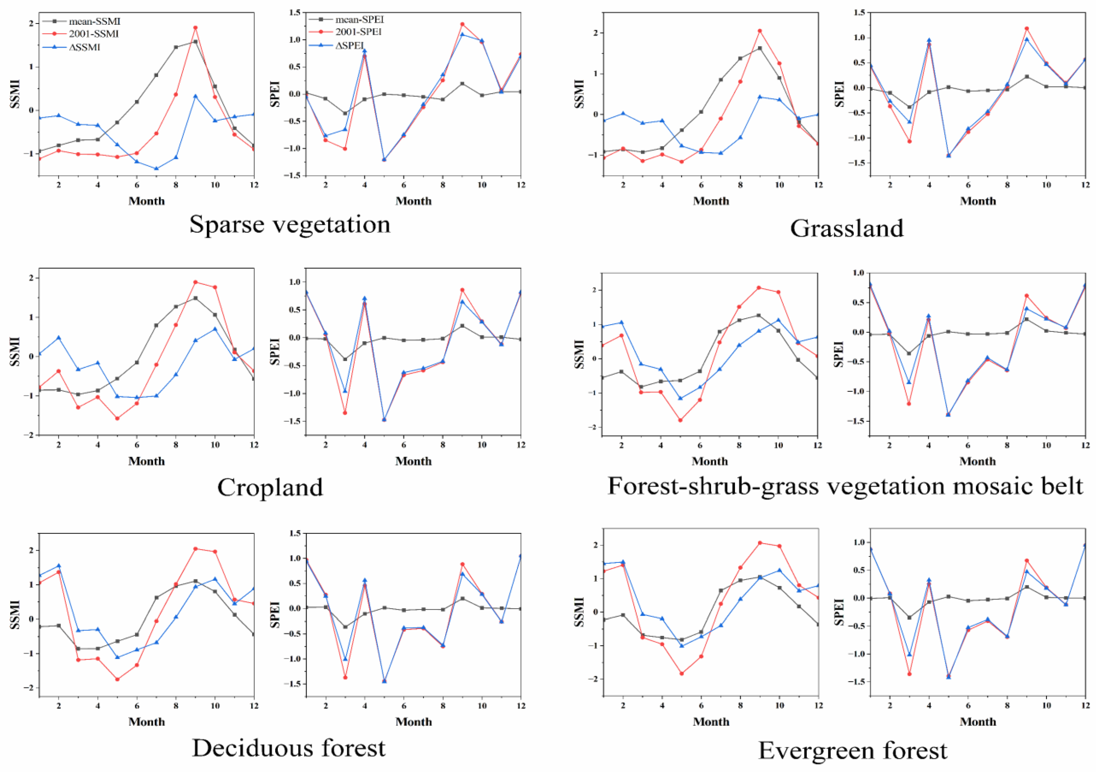
3.4.1. SIF Responds Better Than VIs to Drought

The drought event started in May 2001 and ended in July 2001. These three months were characterized by a severe drop in precipitation compared to the reference year and higher temperatures than the reference year, resulting in a severe lack of soil moisture, which affected the growth of vegetation (Figure 4).

The SPEI drought index indicated that the SPEI for both sparse vegetation and grassland was less than the reference year value from May to July, and drought conditions recovered in August (Figure 9). The cropland, forest-shrub-grass vegetation mosaic belt, deciduous forest, and evergreen forest were all smaller than the multi-year average from May to August before drought conditions subsided in September. The SSMI drought index indicated that sparse vegetation was smaller than the multi-year average from the beginning of the year for SSMI values, and other land classes were less than the multi-annual average from March. Sparse vegetation, grassland, and cropland showed relief in September; forest-shrub-grass vegetation mosaic belts, deciduous forests, and evergreen forests showed relief in August. Both SPEI and SSMI had their lowest values in May, with the largest differences occurring almost simultaneously (Figure 9).

The response of VIs and SIF to drought is reflected by the difference between the VIs and SIF drought year and the reference year. Both VIs and SIF were essentially lower than multi-year averages in 2001, which differed from the drought index performance. During the drought event, the maximum difference between VIs and SIF for sparse vegetation and grassland occurred in May; the maximum difference for forest-shrub-grass vegetation mosaic belt, deciduous and evergreen forests occurred in June (Figure 10), one month after the maximum difference in the drought index. The drought event was caused by a sharp drop in precipitation in March and May 2001. At this time, only SIF showed a clear downward trend, while the change in VIs was much less significant than SIF (Figure 10). In this drought event, both VIs and SIF were subjected to drought stress at the stage of the year when vegetation growth was at its peak, but SIF captured the drought signals and drought initiation stage more accurately.

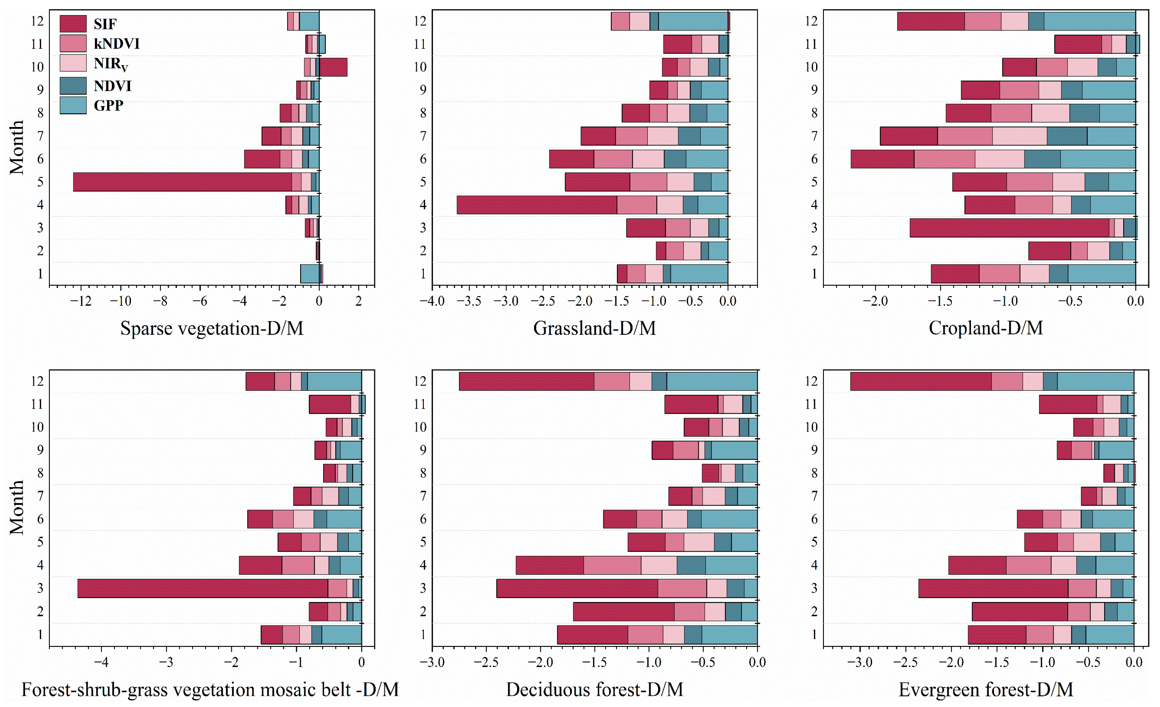
3.4.2. Capture of GPP Changes by VIs and SIF

To further analyze the ability of both to capture GPP loss during drought events, we examined the trends, expressed as a ratio of difference to mean (Figure 10). In sparse vegetation, GPP decreased by 16.19% in May while SIF decreased by more than ten times the multi-year mean, GPP decreased by 53.72% in June while SIF decreased by 179.19%, and GPP decreased by 47.39% in July while SIF decreased by 95.74%. In grassland, SIF changes were not as strong as in sparse vegetation, but SIF still showed the worst performance (except in June when it outperformed NDVI and NIR_V). In cropland, probably due to anthropogenic influence, SIF started to capture GPP loss slightly better than NDVI. As the productivity of the land type increased, SIF gradually outperformed VIs. For example, in deciduous forests, the trend of SIF change in June and July was significantly closer to the trend of GPP change, followed by NIR_V. It can be seen that SIF does not perform as well as kNDVI and NIR_V in areas with low productivity and low vegetation cover during drought events.

We evaluated the magnitude and spatial distribution of the anomalies of VIs and SIF from May to July 2001 (Figure 11). From the spatial distribution of anomalies, VIs, and SIF were basically in moderate negative anomalies. Negative anomalies appeared in May, and strong negative anomalies of the three VIs were mainly distributed in cropland in Shaanxi and Shanxi. The SIF shows strong negative anomalies not only in the cropland but also in the grassland northwest of the Loess Plateau. In June, the negative anomalies are more extensive and strong, with strong negative anomalies in most areas of the Loess Plateau. In July, the negative anomalies are slightly reduced, with strong negative anomalies mainly in Inner Mongolia, Shaanxi, and Shanxi. Compared with the VIs, the negative anomalies of SIF are more serious, especially in June when SIF reaches strong negative anomalies in the forest-shrub-grass vegetation mosaic belt, deciduous forests, and evergreen forests. In general, the anomalies in the east were more severe than those in the west. A large part of the Gansu territory remained normal in these three months.

To further understand the capture of anomalies by VIs and SIF, the relationship between anomalies of VIs and SIF and GPP anomalies was also explored (Figure 12). The capture of anomalies was best for kNDVI (meanR² = 0.50), followed by NIR_V (meanR² = 0.37), NDVI (meanR² = 0.35), and SIF (meanR² = 0.26), which was the poorest performer among the four indices. Specifically, kNDVI was the best performer in all land classes except in sparse vegetation, where NIR_V and NDVI outperformed kNDVI. Even though the other indices were very low in both deciduous and evergreen forests, kNDVI still had a high correlation NIR_V (meanR² = 0.35 and 0.42). We found this to be a significant departure from the initial hypothesis (that SIF would perform better).

4. Discussion

4.1. Changing Trends in the Loess Plateau

In this paper, we used drought index, VIs (NDVI, NIR_V, and kNDVI), SIF, and GPP data to analyze the trends of drought, greening, and GPP in the Loess Plateau from 2001 to 2020. The results found that the drought on the Loess Plateau from 2001 to 2020 showed a decreasing trend, similar to the past studies on the spatial and temporal variations of drought on the Loess Plateau. Su et al. (2023) [60] investigated the characteristics of drought changes on the Loess Plateau and its influencing factors from 2001 to 2020 by using the Crop Water Stress Index (CWSI) and found that the drought on the Loess Plateau showed a downward trend. Hou et al. (2021) [61] used the SPEI and found that it showed a decreasing trend from 1986 to 2019, and the drought characteristics after 2001 were similar to this paper. Zhu et al. (2023) [62] found that the arid and semi-arid zones in China have shown a wetting trend over the past 50 years. However, in this paper, it was found that SSMI showed an increasing trend of drought in deciduous and evergreen forests, which may be due to the increase in forested land area under the Grain for Green Project, the high water demand for forest trees and the high transpiration, which consumed a large amount of soil moisture. Therefore, when implementing the ecological restoration policy, it should be adapted to the local conditions so as to make forests and grasses suitable for forests and grasses. Blindly planting forests and grasses will make the ecosystem more unstable and reduce its self-regulation ability. The greening trend of the entire Loess Plateau is consistent with previous studies [38,39,40]. Since 2000, the greening of the Loess Plateau has been on an upward trend.

Among the VIs, SIF, and GPP trends, we found that only SIF and NIR_V reflected the phenomenon that GPP was higher in deciduous forests than in evergreen forests. In the Loess Plateau, almost all of the deciduous forests are broadleaf forests; in the evergreen forests, coniferous forests are dominant. GPP represents the CO₂ fixed by plants, SIF represents the strength of photosynthesis, and NIR_V represents the potential of harvesting light in response to the greenness of the vegetation. Thus, this phenomenon reflects that the photosynthetic fixation capacity, as well as the potential to harvest light, is higher in deciduous broadleaf forests than in evergreen coniferous forests. This provides evidence for the hypothesis that leaves are constructed and displayed in a manner that matches energy absorption and photosynthetic capacity [24,63]. This result also provides evidence that NIR_V can be used instead of SIF to study photosynthesis in vegetation.

4.2. Response of VIs and SIF to Drought

This drought event occurred in the peak growing season of 2001, and both VIs and SIF were subjected to drought stress, but SIF captured the drought signal more precisely. This is because SIF not only responds to the greenness of vegetation but also contains information related to photosynthesis, such as photosynthetically active radiation and environmental factors. This is similar to Zhang et al.’s (2022) [55] study in the eastern foothills of the Taihang Mountains and Qiu et al.’s (2023) [30] crop study in the Midwestern United States. The VIs and SIF were largely lower than the multi-year averages in all months of 2001, which differed from those exhibited using the drought index. This is due to the ecological restoration policies on the Loess Plateau, where vegetation continues to green up, resulting in higher multi-year averages than the 2001 values. This study also found that the response of different land types to drought varied in time, with a lag in the response of vegetation types to drought and taller shrubs showing greater resilience to drought.

In this paper, we find that SPEI fluctuates greatly on short time scales (SPEI_01 and SPEI_03) and slows down with increasing time scales. This is similar to the study of Stefanidis et al. (2023) [64] in Mediterranean oak forests, who found that at shorter time scales (SPEI_03 and SPEI_06), it was more effective in identifying short-term drought events, while longer time scales (SPEI_12 and SPEI_24) were more effective in identifying drought events of lower frequency but longer duration. The SPEI and SSMI differed in April 2001, with the SPEI recovering to near the multi-year average in April, while the SSMI remained well below the multi-year average (Figure 9). This is probably due to higher precipitation in April. SPEI is a meteorological drought index, and precipitation has a strong influence on its value. Although there was more precipitation in April than in normal years, the plants started to wake up and needed water for growth, resulting in low soil moisture content. Therefore, the SSMI is still in a drought condition in April.

4.3. GPP with VIs and SIF

4.3.1. Correlation at Different Time Scales

On the whole, SIF was superior to other proxies in tracking seasonal GPP, with NIR_V second. This is similar to the study by Wang et al. (2022) [20] in the western US ecological sub-regions. However, the hypothesis that SIF is stronger than VIs is not entirely correct. The correlation between SIF and GPP in sparse vegetation was not as good as that of VIs in other time scales except summer and autumn (Figure 8). The reason may be that the vegetation cover of sparse vegetation is low, and the real SIF signals received by the satellite are weak, which are seriously affected by the noise signals, resulting in a low signal-to-noise ratio [65,66]. NIR_V and kNDVI solve the background contamination problem and better reflect the vegetation signal [22,23]. Furthermore, SIF performance was also lower than VIs in the non-growing season of forest-shrub-grass vegetation mosaic belt and sparse vegetation and in the summer of deciduous and evergreen forests (Figure 8). The reasons for forest-shrub-grass vegetation mosaic belt and sparse vegetation may be (1) weaker SIF signals and (2) low VIs, SIF, and GPP due to the fact that vegetation basically stops growing in the non-growing season, resulting in a low correlation of GPP with VIs and SIF. The reason for the phenomenon that summer SIF performance in deciduous and evergreen forests is lower than VIs may be due to the dense vegetation canopy in the summer. SIF signal is hampered by the high-density canopy obstruction, resulting in impaired radiative transfer (low escape ratio) [67,68,69], and the information from SIF is not fully transmitted to the satellite. The correlation between summer VIs and GPP was also low for forest land compared to other seasonal scales. The reason for this is that GPP in forest land that is in the summer continues to increase to a large extent, with GPP increasing by more than 10 gcm⁻² in July compared to June in most years. Vegetation greenness does not change much in the summer, resulting in VIs not responding well to changes in GPP in summer. R² has a slight increase in the entire study time scale compared to the removal of winter. In winter, VIs, SIF, and GPP are all low, and if GPP were fitted in winter alone as a correlation with VIs and SIF, the correlation would be very low. However, in the entire study time scale fitting, the winter value made up for the vacancy of low value, and the correlation increased.

4.3.2. Capture during Droughts

The original hypothesis that SIF is superior to VIs was also denied in the capture of GPP changes by VIs and SIF during drought events. In sparse vegetation and grasslands, SIFs were significantly less able to capture GPP changes than VIs. This is similar to the study by Wang et al. (2022) [20] in the Western U.S. ecological sub-regions, where NIR_V consistently outperforms SIF in capturing seasonal changes in GPP at low-productivity sites such as sparse herbaceous and sparse shrubby sites. In sparse vegetation and grasslands, we also found that SIF decreased very much during drought events, which could be attributed to low productivity land classes in the first place. Another reason is that GPP increases faster than SIF from spring to summer due to the increase in temperature [70]. This, plus the drought, makes the value of SIF even smaller.

In the capture of GPP anomalies by VIs and SIF during drought events, we find that kNDVI performs best, NIR_V and NDVI followed, and SIF worst. This is at variance with Qiu et al.’s (2023) [30] study of crop productivity in the Midwestern U.S., where they found that GOSIF could better capture yield anomalies of corn and soybean during drought compared with EVI and NIR_V. The reason may be that the vegetation cover in the Loess Plateau is relatively sparse, and SIF is more affected by the noise signal in the low vegetation cover area. Moreover, this drought event occurred during the peak season of vegetation growth, and the escape ratio of the SIF signal in tall shrubs was low, which ultimately led toSIF’s weaker ability to capture anomalies than VIs. We also found that the anomalies correlation showed a significant decrease in the land use types, which were forest-shrub-grass vegetation mosaic belt, deciduous forest, and evergreen forest. This may be due to the relatively large spatial variation in the production of GPP by shrubby vegetation types. kNDVI was initially designed to solve the nonlinearity problem between NDVI and GPP. In anomaly capture, the spatial heterogeneity is strong, and the nonlinearity problem is prominent.

All in all, SIF outperforms VIs most of the time and in most regions, probably because it contains information related to photosynthesis. However, there are still times and regions that SIF does not solve well. Until SIF is able to solve these problems well, it is still necessary to combine VIs to solve multiple problems. SIF should especially pay attention to the integration with NIR_V and kNDVI. NIR_V performs better in the low vegetation cover and low productivity land classes, and kNDVI solves the problem of spatial heterogeneity better. This is very important for improving satellite monitoring of GPP changes, which will be very helpful for future agricultural production, vegetation greening, and carbon neutralization.

5. Conclusions

In this paper, we analyzed the trends of drought, vegetation greening, and GPP in the Loess Plateau from 2001 to 2020 using SPEI, SM, VIs, SIF, and GPP data, and we analyzed the relationship between the two types of indices (VIs and SIF) and GPP in different time scales and during drought. The main conclusions are as follows:

(1)

Based on the spatial and temporal changes of SPEI and SSMI from 2001 to 2020, it was found that the overall drought in the Loess Plateau showed a decreasing trend. However, in the forest, SSMI showed an increasing drought trend. May–July 2001 was identified as a drought event.

(2)

The trends of changes in VIs, SIF, and GPP from 2001 to 2020 are basically the same, and all of them show an upward trend. However, only SIF and NIR_V reflected the phenomenon that the GPP of deciduous forests was higher than that of evergreen forests.

(3)

Both VIs and SIF were subjected to drought stress during the peak vegetation growth season during drought events, but SIF more accurately captured drought signals and the initial stages of drought.

(4)

In the relationship of GPP with VIs and SIF at different time scales, SIF (meanR² = 0.85) performed the best, followed in descending order by NIR_V (meanR² = 0.84), NDVI (meanR² = 0.76), and kNDVI (meanR² = 0.74). Notably, it is worth noting that kNDVI performs best in sparse vegetation (meanR² = 0.85). NIR_V is the most stable of the three VIs and is closest to SIF.

(5)

In the capture of GPP by VIs and SIF during drought, NIR_V and kNDVI performed better in the land classes with low productivity; with the increase in land use classes productivity, SIF showed better capturing ability. In addition, the capture of GPP anomalies was best for kNDVI (meanR² = 0.50), followed by NIR_V (meanR² = 0.37), NDVI (meanR² = 0.35), and SIF (meanR² = 0.26).

Our results suggest that using a single vegetation proxy to characterize the vegetation dynamics of a region may lead to biased GPP estimates in some areas within the region. Therefore, this paper suggests that when integrating different proxies as well as methods, the heterogeneity of vegetation should also be carefully considered in order to respond to regional vegetation dynamics more accurately.

References

1. Beer, C.; Reichstein, M.; Tomelleri, E.; Ciais, P.; Jung, M.; Carvalhais, N.; Rödenbeck, C.; Arain, M.A.; Baldocchi, D.; Bonan, G.B.; et al. Terrestrial Gross Carbon Dioxide Uptake: Global Distribution and Covariation with Climate. Science 2010, 329, 834–838. [Google Scholar] [CrossRef]
2. Anav, A.; Friedlingstein, P.; Beer, C.; Ciais, P.; Harper, A.; Jones, C.; Murray-Tortarolo, G.; Papale, D.; Parazoo, N.C.; Peylin, P.; et al. Spatiotemporal Patterns of Terrestrial Gross Primary Production: A Review. Rev. Geophys. 2015, 53, 785–818. [Google Scholar] [CrossRef]
3. Rockström, J.; Steffen, W.; Noone, K.; Persson, Å.; Chapin, F.S.; Lambin, E.F.; Lenton, T.M.; Scheffer, M.; Folke, C.; Schellnhuber, H.J.; et al. A Safe Operating Space for Humanity. Nature 2009, 461, 472–475. [Google Scholar] [CrossRef]
4. Running, S.W. A Measurable Planetary Boundary for the Biosphere. Science 2012, 337, 1458–1459. [Google Scholar] [CrossRef]
5. Chen, C.; Park, T.; Wang, X.; Piao, S.; Xu, B.; Chaturvedi, R.K.; Fuchs, R.; Brovkin, V.; Ciais, P.; Fensholt, R.; et al. China and India Lead in Greening of the World through Land-Use Management. Nat. Sustain. 2019, 2, 122–129. [Google Scholar] [CrossRef]
6. Piao, S.; Wang, X.; Park, T.; Chen, C.; Lian, X.; He, Y.; Bjerke, J.W.; Chen, A.; Ciais, P.; Tømmervik, H.; et al. Characteristics, Drivers and Feedbacks of Global Greening. Nat. Rev. Earth Environ. 2019, 1, 14–27. [Google Scholar] [CrossRef]
7. Yang, Y.; Shi, Y.; Sun, W.; Chang, J.; Zhu, J.; Chen, L.; Wang, X.; Guo, Y.; Zhang, H.; Yu, L.; et al. Terrestrial Carbon Sinks in China and around the World and Their Contribution to Carbon Neutrality. Sci. China Life Sci. 2022, 65, 861–895. [Google Scholar] [CrossRef] [PubMed]
8. Yang, Y.; Roderick, M.L.; Guo, H.; Miralles, D.G.; Zhang, L.; Fatichi, S.; Luo, X.; Zhang, Y.; McVicar, T.R.; Tu, Z.; et al. Evapotranspiration on a Greening Earth. Nat. Rev. Earth Environ. 2023, 4, 626–641. [Google Scholar] [CrossRef]
9. Shao, D.; Chen, S.; Tan, X.; Gu, W. Drought Characteristics over China during 1980–2015. Int. J. Climatol. 2018, 38, 3532–3545. [Google Scholar] [CrossRef]
10. Zhao, Z.; Zhang, B.; Pan, L.; Niu, P.; Guo, J. Diagnosis and Prediction of Drought in Eastern Inner Mongolia Based on SPEI. Environ. Ecol. 2023, 5, 39–48. [Google Scholar]
11. Zeng, Z.; Wu, W.; Li, Y.; Huang, C.; Zhang, X.; Peñuelas, J.; Zhang, Y.; Gentine, P.; Li, Z.; Wang, X.; et al. Increasing Meteorological Drought under Climate Change Reduces Terrestrial Ecosystem Productivity and Carbon Storage. One Earth 2023, 6, 1326–1339. [Google Scholar] [CrossRef]
12. World Meteorological Organization (WMO). Drought Monitoring and Early Warning: Concepts, Progress and Future Challenges; WMO No. 1006; World Meteorological Organization (WMO): Geneva, Switzerland, 2006; Available online: http://www.wamis.org/agm/pubs/brochures/WMO1006e.pdf (accessed on 30 January 2024).
13. Xu, M.; Zhang, T.; Zhang, Y.; Chen, N.; Zhu, J.; He, Y.; Zhao, T.; Yu, G. Drought Limits Alpine Meadow Productivity in Northern Tibet. Agric. For. Meteorol. 2021, 303, 108371. [Google Scholar] [CrossRef]
14. Zhao, M.; Running, S.W. Response to Comments on “Drought-Induced Reduction in Global Terrestrial Net Primary Production from 2000 through 2009”. Science 2011, 333, 1093. [Google Scholar] [CrossRef]
15. Frank, D.; Reichstein, M.; Bahn, M.; Thonicke, K.; Frank, D.; Mahecha, M.D.; Smith, P.; Van Der Velde, M.; Vicca, S.; Babst, F.; et al. Effects of Climate Extremes on the Terrestrial Carbon Cycle: Concepts, Processes and Potential Future Impacts. Glob. Change Biol. 2015, 21, 2861–2880. [Google Scholar] [CrossRef]
16. Piao, S.; He, Y.; Wang, X.; Chen, F. Estimation of China’s terrestrial ecosystem carbon sink: Methods, progress and prospects. Sci. China Earth Sci. 2022, 65, 641–651. [Google Scholar] [CrossRef]
17. Baldocchi, D.; Falge, E.; Gu, L.; Olson, R.; Hollinger, D.; Running, S.; Anthoni, P.; Bernhofer, C.; Davis, K.; Evans, R.; et al. FLUXNET: A New Tool to Study the Temporal and Spatial Variability of Ecosystem–Scale Carbon Dioxide, Water Vapor, and Energy Flux Densities. Bull. Am. Meteorol. Soc. 2001, 82, 2415–2434. [Google Scholar] [CrossRef]
18. Qiu, R.; Han, G.; Ma, X.; Xu, H.; Shi, T.; Zhang, M. A Comparison of OCO-2 SIF, MODIS GPP, and GOSIF Data from Gross Primary Production (GPP) Estimation and Seasonal Cycles in North America. Remote Sens. 2020, 12, 258. [Google Scholar] [CrossRef]
19. Khalifa, M.; Elagib, N.A.; Ribbe, L.; Schneider, K. Spatio-Temporal Variations in Climate, Primary Productivity and Efficiency of Water and Carbon Use of the Land Cover Types in Sudan and Ethiopia. Sci. Total Environ. 2018, 624, 790–806. [Google Scholar] [CrossRef]
20. Wang, X.; Biederman, J.A.; Knowles, J.F.; Scott, R.L.; Turner, A.J.; Dannenberg, M.P.; Köhler, P.; Frankenberg, C.; Litvak, M.E.; Flerchinger, G.N.; et al. Satellite Solar-Induced Chlorophyll Fluorescence and near-Infrared Reflectance Capture Complementary Aspects of Dryland Vegetation Productivity Dynamics. Remote Sens. Environ. 2022, 270, 112858. [Google Scholar] [CrossRef]
21. Huang, X.; Xiao, J.; Ma, M. Evaluating the Performance of Satellite-Derived Vegetation Indices for Estimating Gross Primary Productivity Using FLUXNET Observations across the Globe. Remote Sens. 2019, 11, 1823. [Google Scholar] [CrossRef]
22. Badgley, G.; Field, C.B.; Berry, J.A. Canopy Near-Infrared Reflectance and Terrestrial Photosynthesis. Sci. Adv. 2017, 3, e1602244. [Google Scholar] [CrossRef]
23. Camps-Valls, G.; Campos-Taberner, M.; Moreno-Martínez, Á.; Walther, S.; Duveiller, G.; Cescatti, A.; Mahecha, M.D.; Muñoz-Marí, J.; García-Haro, F.J.; Guanter, L.; et al. A Unified Vegetation Index for Quantifying the Terrestrial Biosphere. Sci. Adv. 2021, 7, eabc7447. [Google Scholar] [CrossRef]
24. Badgley, G.; Anderegg, L.D.L.; Berry, J.A.; Field, C.B. Terrestrial Gross Primary Production: Using NIR V to Scale from Site to Globe. Glob. Chang. Biol. 2019, 25, 3731–3740. [Google Scholar] [CrossRef] [PubMed]
25. Frankenberg, C.; Fisher, J.B.; Worden, J.; Badgley, G.; Saatchi, S.S.; Lee, J.-E.; Toon, G.C.; Butz, A.; Jung, M.; Kuze, A.; et al. New Global Observations of the Terrestrial Carbon Cycle from GOSAT: Patterns of Plant Fluorescence with Gross Primary Productivity. Geophys. Res. Lett. 2011, 38, 17. [Google Scholar] [CrossRef]
26. Frankenberg, C.; O’Dell, C.; Berry, J.; Guanter, L.; Joiner, J.; Köhler, P.; Pollock, R.; Taylor, T.E. Prospects for Chlorophyll Fluorescence Remote Sensing from the Orbiting Carbon Observatory-2. Remote Sens. Environ. 2014, 147, 1–12. [Google Scholar] [CrossRef]
27. Joiner, J.; Guanter, L.; Lindstrot, R.; Voigt, M.; Vasilkov, A.P.; Middleton, E.M.; Huemmrich, K.F.; Yoshida, Y.; Frankenberg, C. Global Monitoring of Terrestrial Chlorophyll Fluorescence from Moderate-Spectral-Resolution near-Infrared Satellite Measurements: Methodology, Simulations, and Application to GOME-2. Atmos. Meas. Tech. 2013, 6, 2803–2823. [Google Scholar] [CrossRef]
28. Li, X.; Xiao, J. A Global, 0.05-Degree Product of Solar-Induced Chlorophyll Fluorescence Derived from OCO-2, MODIS, and Reanalysis Data. Remote Sens. 2019, 11, 517. [Google Scholar] [CrossRef]
29. Sun, Y.; Frankenberg, C.; Wood, J.D.; Schimel, D.S.; Jung, M.; Guanter, L.; Drewry, D.T.; Verma, M.; Porcar-Castell, A.; Griffis, T.J.; et al. OCO-2 Advances Photosynthesis Observation from Space via Solar-Induced Chlorophyll Fluorescence. Science 2017, 358, eaam5747. [Google Scholar] [CrossRef]
30. Qiu, R.; Li, X.; Han, G.; Xiao, J.; Ma, X.; Gong, W. Monitoring Drought Impacts on Crop Productivity of the U.S. Midwest with Solar-Induced Fluorescence: GOSIF Outperforms GOME-2 SIF and MODIS NDVI, EVI, and NIRV. Agric. For. Meteorol. 2022, 323, 109038. [Google Scholar] [CrossRef]
31. Daumard, F.; Champagne, S.; Fournier, A.; Goulas, Y.; Ounis, A.; Hanocq, J.-F.; Moya, I. A Field Platform for Continuous Measurement of Canopy Fluorescence. IEEE Trans. Geosci. Remote Sens. 2010, 48, 3358–3368. [Google Scholar] [CrossRef]
32. Flexas, J.; Escalona, J.M.; Evain, S.; Gulías, J.; Moya, I.; Osmond, C.B.; Medrano, H. Steady-state Chlorophyll Fluorescence (Fs) Measurements as a Tool to Follow Variations of Net CO 2 Assimilation and Stomatal Conductance during Water-stress in C 3 Plants. Physiol. Plant. 2002, 114, 231–240. [Google Scholar] [CrossRef]
33. Dobrowski, S.; Pushnik, J.; Zarcotejada, P.; Ustin, S. Simple Reflectance Indices Track Heat and Water Stress-Induced Changes in Steady-State Chlorophyll Fluorescence at the Canopy Scale. Remote Sens. Environ. 2005, 97, 403–414. [Google Scholar] [CrossRef]
34. Wang, C.; Wu, X.; Fu, B.; Han, X.; Chen, Y.; Wang, K.; Zhou, H.; Feng, X.; Li, Z. Ecological restoration in the key ecologically vulnerable regions: Current situation and development direction. Acta Ecol. Sin. 2019, 39, 7333–7343. [Google Scholar] [CrossRef]
35. Fu, B.; Wu, X.; Wang, Z.; Wu, X.; Wang, S. Coupling Human and Natural Systems for Sustainability: Experience from China’s Loess Plateau. Earth Syst. Dyn. 2022, 13, 795–808. [Google Scholar] [CrossRef]
36. Fu, B.; Wang, S.; Liu, Y.; Liu, J.; Liang, W.; Miao, C. Hydrogeomorphic Ecosystem Responses to Natural and Anthropogenic Changes in the Loess Plateau of China. Annu. Rev. Earth Planet. Sci. 2017, 45, 223–243. [Google Scholar] [CrossRef]
37. Bryan, B.A.; Gao, L.; Ye, Y.; Sun, X.; Connor, J.D.; Crossman, N.D.; Stafford-Smith, M.; Wu, J.; He, C.; Yu, D.; et al. China’s Response to a National Land-System Sustainability Emergency. Nature 2018, 559, 193–204. [Google Scholar] [CrossRef]
38. Yu, Y.; Zhao, W.; Martinez-Murillo, J.F.; Pereira, P. Loess Plateau: From Degradation to Restoration. Sci. Total Environ. 2020, 738, 140206. [Google Scholar] [CrossRef] [PubMed]
39. Naeem, S.; Zhang, Y.; Zhang, X.; Tian, J.; Abbas, S.; Luo, L.; Meresa, H.K. Both Climate and Socioeconomic Drivers Contribute to Vegetation Greening of the Loess Plateau. Sci. Bull. 2021, 66, 1160–1163. [Google Scholar] [CrossRef] [PubMed]
40. Wu, X.; Wang, S.; Fu, B.; Feng, X.; Chen, Y. Socio-Ecological Changes on the Loess Plateau of China after Grain to Green Program. Sci. Total Environ. 2019, 678, 565–573. [Google Scholar] [CrossRef]
41. Sun, Y.; Liu, X.; Ren, Z.; Li, S. Spatiotemporal Variations of Multi-Scale Drought and Its Influencing Factors across the Loess Plateau from 1960 to 2016. Geogr. Res. 2019, 38, 1820–1832. [Google Scholar]
42. Wang, Y.; Shi, H.; Jiang, Y.; Wu, Y.; Gao, Y.; Ding, C. Spatio-Temporal Variation of Drought Characteristics and Its Influence Factors in Loess Plateau Based on TVDI. Trans. Chin. Soc. Agric. Mach. 2023, 54, 184–196. [Google Scholar] [CrossRef]
43. Li, Y. Spatiotemporal Changes and Influencing Factors of Vegetation Cover on the Loess Plateau from 2000 to 2018. Sci. Soil Water Conserv. 2021, 19, 60–84. [Google Scholar] [CrossRef]
44. Zastrow, M. China’s Tree-Planting Drive Could Falter in a Warming World. Nature 2019, 573, 474–475. [Google Scholar] [CrossRef]
45. Cao, Y.Q.; Zhou, S.H.; Yang, X.T. Vegetation dynamics and its response to climate change in Liaoning Province in last 20 years. Acta Ecol. Sin. 2022, 42, 5966–5979. [Google Scholar] [CrossRef]
46. Vicente-Serrano, S.M.; Beguería, S.; López-Moreno, J.I.; Angulo, M.; El Kenawy, A. A New Global 0.5° Gridded Dataset (1901–2006) of a Multiscalar Drought Index: Comparison with Current Drought Index Datasets Based on the Palmer Drought Severity Index. J. Hydrometeorol. 2010, 11, 1033–1043. [Google Scholar] [CrossRef]
47. Xia, H.; Zhao, X.; Zhao, W. High-Resolution SPEI Dataset for Drought Monitoring and Impact Analysis in Mainland China from 2001 to 2020. Natl. Ecosyst. Data Bank 2023. [Google Scholar] [CrossRef]
48. Vicente-Serrano, S.M.; Beguería, S.; López-Moreno, J.I. A Multiscalar Drought Index Sensitive to Global Warming: The Standardized Precipitation Evapotranspiration Index. J. Clim. 2010, 23, 1696–1718. [Google Scholar] [CrossRef]
49. Roderick, M.L.; Greve, P.; Farquhar, G.D. On the Assessment of Aridity with Changes in Atmospheric CO2. Water Resour. Res. 2015, 51, 5450–5463. [Google Scholar] [CrossRef]
50. Greve, P.; Roderick, M.L.; Ukkola, A.M.; Wada, Y. The Aridity Index under Global Warming. Environ. Res. Lett. 2019, 14, 124006. [Google Scholar] [CrossRef]
51. Zhou, H.K.; Wu, J.J.; Li, X.H.; Liu, L.Z.; Yang, J.H.; Han, X.Y. Suitability of Assimilated Data-Based Standardized Soil Moisture Index for Agricultural Drought Monitoring. Acta Ecol. Sin. 2019, 39, 2191–2202. [Google Scholar] [CrossRef]
52. Zheng, C.; Jia, L.; Zhao, T. A 21-Year Dataset (2000–2020) of Gap-Free Global Daily Surface Soil Moisture at 1-km Grid Resolution. Sci. Data 2023, 10, 139. [Google Scholar] [CrossRef]
53. Grades of Meteorological Drought. China Meteorological Administration (CMA). Available online: https://opehttps://openstd.samr.gov.cn/bzgk/gb/index (accessed on 30 October 2023).
54. Li, Y.; Li, M.; Zheng, Z.; Shen, W.; Li, Y.; Rong, P.; Qin, Y. Trends in Drought and Effects on Carbon Sequestration over the Chinese Mainland. Sci. Total Environ. 2023, 856, 159075. [Google Scholar] [CrossRef]
55. Zhang, T.; Zhou, J.; Yu, P.; Li, J.; Kang, Y.; Zhang, B. Response of Ecosystem Gross Primary Productivity to Drought in Northern China Based on Multi-Source Remote Sensing Data. J. Hydrol. 2023, 616, 128808. [Google Scholar] [CrossRef]
56. Fuller, D.O.; Wang, Y. Recent Trends in Satellite Vegetation Index Observations Indicate Decreasing Vegetation Biomass in the Southeastern Saline Everglades Wetlands. Wetlands 2014, 34, 67–77. [Google Scholar] [CrossRef]
57. Li, Y.; Qin, Y.; Rong, P. Evolution of Potential Evapotranspiration and Its Sensitivity to Climate Change Based on the Thornthwaite, Hargreaves, and Penman–Monteith Equation in Environmental Sensitive Areas of China. Atmos. Res. 2022, 273, 106178. [Google Scholar] [CrossRef]
58. Hao, Y.; Baik, J.; Fred, S.; Choi, M. Comparative Analysis of Two Drought Indices in the Calculation of Drought Recovery Time and Implications on Drought Assessment: East Africa’s Lake Victoria Basin. Stoch. Environ. Res. Risk Assess. 2022, 36, 1943–1958. [Google Scholar] [CrossRef]
59. Eklund, L.; Seaquist, J. Meteorological, Agricultural and Socioeconomic Drought in the Duhok Governorate, Iraqi Kurdistan. Nat. Hazards 2015, 76, 421–441. [Google Scholar] [CrossRef]
60. Su, W.; Yang, Y.; Wang, T. Variation Characteristics and Influencing Factors of Drought in the Loess Plateau in Recent 20 Years. Sci. Technol. Eng. 2023, 23, 4551–4560. [Google Scholar]
61. Hou, Q.-Q.; Pei, T.-T.; Chen, Y. Variations of Drought and Its Trend in the Loess Plateau from 1986 to 2019. Chin. J. Appl. Ecol. 2021, 32, 649–660. [Google Scholar] [CrossRef]
62. Zhu, B.; Zhang, Q.; Huang, P.C.; Yang, J.H.; Hu, J.; Li, C.H. Characteristics of Climate Change in Arid and Semi-Arid Areas of China and Its Influence on Climatic Dry-Wet Fluctuation. Trans. Atmos. Sci. 2023, 46, 42–54. [Google Scholar] [CrossRef]
63. Wang, S.; Zhang, Y.; Ju, W.; Qiu, B.; Zhang, Z. Tracking the Seasonal and Inter-Annual Variations of Global Gross Primary Production during Last Four Decades Using Satellite near-Infrared Reflectance Data. Sci. Total Environ. 2021, 755, 142569. [Google Scholar] [CrossRef]
64. Stefanidis, S.; Rossiou, D.; Proutsos, N. Drought Severity and Trends in a Mediterranean Oak Forest. Hydrology 2023, 10, 167. [Google Scholar] [CrossRef]
65. Guanter, L.; Aben, I.; Tol, P.; Krijger, J.M.; Hollstein, A.; Köhler, P.; Damm, A.; Joiner, J.; Frankenberg, C.; Landgraf, J. Potential of the TROPOspheric Monitoring Instrument (TROPOMI) Onboard the Sentinel-5 Precursor for the Monitoring of Terrestrial Chlorophyll Fluorescence. Atmos. Meas. Tech. 2015, 8, 1337–1352. [Google Scholar] [CrossRef]
66. Köhler, P.; Fischer, W.W.; Rossman, G.R.; Grotzinger, J.P.; Doughty, R.; Wang, Y.; Yin, Y.; Frankenberg, C. Mineral Luminescence Observed from Space. Geophys. Res. Lett. 2021, 48, e2021GL095227. [Google Scholar] [CrossRef]
67. Fournier, A.; Daumard, F.; Champagne, S.; Ounis, A.; Goulas, Y.; Moya, I. Effect of Canopy Structure on Sun-Induced Chlorophyll Fluorescence. ISPRS J. Photogramm. Remote Sens. 2012, 68, 112–120. [Google Scholar] [CrossRef]
68. Van Wittenberghe, S.; Alonso, L.; Verrelst, J.; Moreno, J.; Samson, R. Bidirectional Sun-Induced Chlorophyll Fluorescence Emission Is Influenced by Leaf Structure and Light Scattering Properties—A Bottom-up Approach. Remote Sens. Environ. 2015, 158, 169–179. [Google Scholar] [CrossRef]
69. Zeng, Y.; Badgley, G.; Dechant, B.; Ryu, Y.; Chen, M.; Berry, J.A. A Practical Approach for Estimating the Escape Ratio of Near-Infrared Solar-Induced Chlorophyll Fluorescence. Remote Sens. Environ. 2019, 232, 111209. [Google Scholar] [CrossRef]
70. Chen, A.; Mao, J.; Ricciuto, D.; Lu, D.; Xiao, J.; Li, X.; Thornton, P.E.; Knapp, A.K. Seasonal Changes in GPP/SIF Ratios and Their Climatic Determinants across the Northern Hemisphere. Glob. Change Biol. 2021, 27, 5186–5197. [Google Scholar] [CrossRef]
Figure 1. Technical flow chart.
Forests 15 00339 g001
Figure 2. Overview of the study area (left) and land use cover (right).
Forests 15 00339 g002
Figure 3. Time-varying characteristics of SPEI and SSMI.
Forests 15 00339 g003
Figure 4. Trend changes in aridity indices, GPP, VIs, and SIF from 2001–2020; significance distributions of SPEI, SSMI, GPP, NDVI, NIRV, kNDVI, and SIF, respectively, from (ag).
Forests 15 00339 g004
Figure 5. Trends in precipitation and temperature on the Loess Plateau in 2001 and the reference year.
Forests 15 00339 g005
Figure 6. Spatial distribution of SPEI (a) and SSMI (b) during the drought of 2001.
Forests 15 00339 g006
Figure 7. Interannual variation in VIs, SIF, and GPP.
Forests 15 00339 g007
Figure 8. The correlation between VIs, SIF, and GPP. Sp, Su, Au, Ngs, Gs, Rw, and Am are spring, summer, autumn, non-growing season, growing season, removal of winter, and the entire study period, respectively.
Forests 15 00339 g008
Figure 9. Trends in drought index for 2001 and reference year. Where mean-SSMI and mean-SPEI are monthly averages of SSMI and SPEI from 2000 to 2020; 2001-SSMI and 2001-SPEI are monthly values of SSMI and SPEI for 2001; SSMI and SPEI are the difference between the monthly values of SSMI and SPEI for 2001 and the multi-year average.
Forests 15 00339 g009
Figure 10. Trends in VIs, SIF, and GPP in 2001. D/M is the ratio of the difference to the mean: (2001 value − mean)/mean value.
Forests 15 00339 g010
Figure 11. Spatial distribution of anomalies in VIs and SIF for May, June, and July 2001.
Forests 15 00339 g011
Figure 12. Correlation of GPP anomalies with VIs and SIF anomalies. Sv, Gl, Cl, Fsg, Df, and Ef are sparse vegetation, grassland, cultivated land, forest shrub, deciduous forest, and evergreen forest, respectively.
Forests 15 00339 g012