Forest Cover Change Monitoring Using Sub-Pixel Mapping with Edge-Matching Correction

Abstract

Sentinel-2 serves as a crucial data source for monitoring forest cover change. In this study, a sub-pixel mapping of forest cover is performed on Sentinel-2 images, downscaling the spatial resolution of the positioned results to 2.5 m, enabling sub-pixel-level forest cover monitoring. A novel sub-pixel mapping with edge-matching correction is proposed on the basis of the Sentinel-2 images, combining edge-matching technology to extract the forest boundary of Jilin-1 images at sub-meter level as spatial constraint information for sub-pixel mapping. This approach enables accurate mapping of forest cover, surpassing traditional pixel-level monitoring in terms of accuracy and robustness. The corrected mapping method allows more spatial detail to be restored at forest boundaries, monitoring forest changes at a smaller scale, which is highly similar to actual forest boundaries on the surface. The overall accuracy of the modified sub-pixel mapping method reaches 93.15%, an improvement of 1.96% over the conventional Sub-pixel-pixel Spatial Attraction Model (SPSAM). Additionally, the kappa coefficient improved by 0.15 to reach 0.892 during the correction. In summary, this study introduces a new method of forest cover monitoring, enhancing the accuracy and efficiency of acquiring forest resource information. This approach provides a fresh perspective in the field of forest cover monitoring, especially for monitoring small deforestation and forest degradation activities.

1. Introduction

Forests are found on every continent of the world and are one of the most widespread and complex natural ecosystems on Earth, with significant ecological, environmental, economic and social values [1]. In the Forest Resources Assessment 2020 report, the Food and Agriculture Organization of the United Nations (FAO) presents compelling evidence that the current global forest cover encompasses approximately 4.06 billion ha, equivalent to 31% of Earth’s land area. The global forest area has continued to shrink since 1990, with a net loss of 178 million ha [2]. Continuous monitoring of forest cover is therefore particularly essential. Forest cover monitoring can quantify important information such as forest area, cover, deforestation, and fire incidence, and provide a reliable basis for ecological monitoring [3]. At the same time, it is possible to understand the current situation and development trends of the forest ecological environment and to provide basic data for measures to protect it.

Traditional forest cover monitoring relies on field monitoring, which involves heavy workloads, time-consumption and challenges in keeping the information up to date. In recent years, the rise of satellite remote sensing technology has opened up more possibilities for continuous monitoring of forest cover. The current mainstream methods of monitoring forest cover by satellite remote sensing can be classified as the remote sensing index method [4], image transformation method [5], texture analysis method [6], object-based method [7], machine learning classification method, and so on [8].

The remote sensing index method is a commonly used method for monitoring forest changes. The use of remote sensing data can obtain information on various reflectances of forest vegetation and combine it with several index calculation methods to determine the area covered and the growth state of the forest. Common remote sensing indices include the Normalised Vegetation Index (NDVI) [9], Vegetation Index (VI) [10], Enhanced Vegetation Index (EVI) [11], Difference Normalized Vegetation Index (DVI) [12], etc. These indices are calculated according to the reflectance of different wavelengths and give an effective indication of the condition and growth of the vegetation.

The image change method is a technique based on mathematical transformation, which can perform dimensionality reduction and feature extraction on multispectral or hyperspectral remote sensing images. In forest cover monitoring, the image transformation method can be used to reduce redundant information, highlight forest cover-related features in images, and provide effective feature vectors to aid image classification. For example, principal component analysis (PCA) is used to identify the main factors affecting forest cover [13]; the Karhunen–Loeve transform (KLT) is used to reduce data dimensionality and storage requirements [14]; and the tasseled cap transform (TCT) can mine vegetation change features in time-series data [15].

The texture analysis method is widely used for analyzing, assessing, and monitoring changes in forest ecosystems, providing an efficient and accurate means of forest monitoring. Some commonly used techniques include the grey-level co-occurrence matrix (GLCM) [16] and wavelet transform [17]. The GLCM extracts texture features such as contrast, energy, correlation, and uniformity by calculating statistical information on the occurrence of pixel pairs at different grey levels. On the other hand, the wavelet transform enables the highlighting or suppression of texture information at specific frequencies or scales, facilitating the capture of fine texture structures or extraction of texture information at larger scales. The application of these methods has significantly enhanced the accuracy and reliability of monitoring results.

The object-based method is extensively applied in forest monitoring. These methods utilize a segmentation process that integrates spatial and spectral information to group pixels into homogeneous regions, followed by classification using new object descriptors. These object descriptors can encompass geometric and textural features [18] or temporal features [19]. Such approaches hold significant importance for forest change monitoring by combining spatial and spectral information and partitioning pixels into homogeneous regions prior to classification. Furthermore, the introduction of novel object descriptors enables better representation of characteristics within homogeneous regions, thereby further improving the precision of monitoring results.

Machine learning classification has a wide range of applications in remote sensing monitoring of forest cover. It is a data-driven approach that learns from a large number of training samples of known categories to build a classifier model, which is then applied to new unknown samples for classification [20,21]. Common classifiers include decision tree (DT) [22], maximum-likelihood estimation (MLE) [23], artificial neural network (ANN) [24], support vector machine (SVM) [25], and random forest (RF) [26]. Machine learning classification has higher adaptivity and scalability. It can effectively exploit the rich information in remote sensing data and enable fast classification and accurate determination when processing large-scale remote sensing data.

However, the aforementioned studies on the use of remote sensing technology to monitor forest cover are only at the image level or pixel level. Due to the limitation of spatial resolution and complex land class distribution, there are often a certain number of mixed pixels in remote sensing images, which means that one pixel may contain spectral information of multiple land types [27]. In terms of the pixel-level forest cover monitoring, at the junction of forest and other land types in the image, mixed pixels can only be classified as one of these land classes, which tends to result in the loss of detailed spatial information at the junctions of land classes, posing difficulties to accurately classify and monitor forest cover status. To solve this problem, this study introduces sub-pixel mapping technology into forest cover monitoring research, aiming to pinpoint accurate information of forest cover at the sub-pixel-level and provide a more effective method for monitoring forest cover changes. Most current sub-pixel mapping models are based on Atkinson’s spatial dependence theory. This theory suggests that when the land cover target size is larger than the pixel spatial resolution, the dependence between pixels and neighboring sub-pixels is inversely proportional to their distance from each other. The Hopfield neural network (HNN) based sub-pixel mapping method is one of the first methods proposed. The method was introduced by Tatem to derive the sub-pixel mapping by building a neural network model based on the dependence between neighboring pixels [28]. Subsequently, Atkinson proposed the pixel swapping algorithm (PSA), which obtains the optimal sub-pixel mapping results by iteration. The algorithm uses the dependence coefficients between the sub-pixels and the neighboring sub-pixels in the mixed pixel to select the sub-pixels to be swapped, thus optimizing the spatial correlation of the swapped images [29]. Mertens proposed the sub-pixel-pixel spatial attraction model (SPSAM). The model uses the spatial dependence between a sub-pixel and a neighboring mixed pixel as a reference criterion for sub-pixel mapping. The method is based on physical meaning and combines spatial information and image semantics to improve the accuracy and efficiency of sub-pixel mapping [30]. Dr. Kasetkasem introduced the theory of the Markov random field (MRF) into the sub-pixel mapping method, which allows sub-pixel mapping results to be not entirely constrained by abundance through considering both spectral information and spatial dependence information of land classes [31]. In recent years, sub-pixel mapping methods based on swarm intelligence theory have also emerged as a new research direction for processing multitemporal remote sensing image [32]. Sub-pixel mapping is applied to water extraction [33], impermeable surface extraction [34], forest fire monitoring [35], burned area extraction [36], forest-fire smoke detection [37], etc. Jiang proposes a sub-pixel surface water mapping method based on morphological expansion and erosion operations and Markov random field (DE_MRF) to predict 2 m resolution surface water maps of heterogeneous regions from Sentinel-2 images [38]. Li presents a method to improve the accuracy of sub-pixel mapping of wetland floods based on random forest and spatial attraction model (RFSAM) remote sensing imagery, achieving more accurate sub-pixel mapping results in the visual and quantitative assessment of two wetlands floods [39]. Chen indicates a method for mapping impervious surfaces using Sentinel-2 time series and determining the exact spatial location of impervious surfaces within each pixel [40]. Xu produces a sub-pixel mapping model incorporating a pixel-swapping algorithm for timely monitoring of forest fire sources [41]. Xu shows a Burned-Area Subpixel Mapping (BASM) workflow to position fire-trail areas at the sub-pixel-level [42]. Li X improves sub-pixel mapping results based on random forest classification results for forest fire smoke identification and sub-pixel positioning [43].

Although sub-pixel mapping is applied in many of these fields, sub-pixel-level forest cover monitoring is rare. This is due to the fact that the shape of forest edges is often irregular, and that the lack of information on forest boundary constraints makes it difficult to position forest boundaries accurately, which threatens the accuracy of forest cover monitoring, while the edge-matching technique can effectively constrain the boundary information in remote sensing mapping [44,45,46]. In order to position the forest in the mixed pixel accurately, to map the forest cover at sub-pixel-level and enable monitoring of subtle changes in forests at small scales, this study proposes forest cover change monitoring using sub-pixel mapping with edge-matching correction.

Firstly, five different classifiers are used to classify and monitor Sentinel-2 images to analyze the accuracy of pixel-level monitoring. Secondly, a mixed pixel decomposition is performed on the Sentinel-2 images to solve for the abundance information of each class of endmember in the mixed pixel. Then, the spatial distribution is positioned by sub-pixel mapping. Next, refinement of the monitoring results is carried out by combining the edge-matching algorithm to correct for the loss of spatial information at the forest boundary due to the lack of constraint information. Finally, the pixel-level monitoring results are compared with the sub-pixel-level monitoring results before and after correction by means of a confusion matrix.

2. Materials and Methods

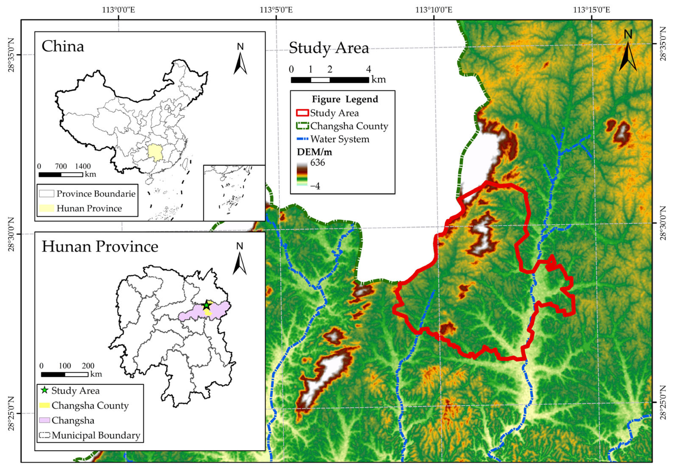
2.1. Study Area

Qingshanpu Town is located in the northwest of Changsha County, Hunan Province. As shown in Figure 1, its topography is slightly high in the north and low in the south, and the terrain is divided into mountains and hills. It has a humid subtropical monsoon climate with an average annual temperature of 18 °C and average temperatures of 4.6 °C in January and 29.7 °C in July. The average annual frost-free period is 275 days. The average annual sunshine hours are 1300–1800, and the average annual precipitation is 1200–1500 mm. The total population is 18,244. Qingshanpu Town covers an area of 46.19 km², with 1220 ha of arable land (including 1186.66 ha of paddy fields), 230.66 ha of water surface, and 2133.33 ha of mountainous land. The existing forest land is more than 1762.25 ha, with a forest coverage rate of 40%, total number of trees of 2,745,243, and total volume of storage of 521,530.2 cubic meters. The dominant tree species in the area is the horsetail pine, which has an average diameter at breast height of 14 cm and an average height of 9 m.

2.2. Data Resources and Data Pre-Processing

In this study, Sentinel-2 images are selected as the primary data source for the forest change monitoring experiment, while SuperView-1 images are utilized for accuracy verification, and Jilin-1 images are used for edge-matching and corrected sub-pixel mapping result. All three images are projected in UTM-WGS 1984 coordinate system. The Sentinel-2 data are acquired from the United States Geological Survey (USGS) website (https://www.usgs.gov/, accessed on 25 April 2023) and are provided at L2A level. On the other hand, the Jilin-1 data and SuperView-1 data are obtained from the Yun Yao satellite website (https://www.img.net/, accessed on 28 April 2023) and are available at L1 level.

Both Sentinel-2 and Jilin-1 images were collected on 12 January 2021, and High View imagery was collected on 18 February 2021. The images were collected in the winter in the study area, which can reflect forest cover to the greatest extent possible, reduce confusion between forest and grassland and other land types, All images cover the entire study area, and contain less than 5% cloud.

Environment for Visualizing Images 5.3 (ENVI 5.3) is used to pre-process the SuperView-1 data and Jilin-1 data, is used to pre-process the Jilin-1 data, including radiometric calibration, atmospheric correction, and image fusion. For Sentinel-2 data, as they can be directly acquired at the L2A level, they have already undergone a series of pre-processing, such as atmospheric correction, geometric correction, brightness equalization, etc. In this study, Sentinel Application Platform (SNAP) is used to perform band extraction, image registration, and resampling on Sentinel-2. The selected bands of Sentinel 2, SuperView-1 and Jilin 1 satellite image data are shown in

Table 1. Selected bands of Sentinel 2, SuperView-1 and Jilin-1 satellite image data sets used in the current study.

Satellite	Sensor	Band Number	Central Wavelength (µm)	Spatial Resolution (m)
Sentinel-2	MSI	B2	0.49	10
		B3	0.56	10
		B4	0.67	10
		B5	0.70	20
		B6	0.74	20
		B7	0.78	20
		B8	0.84	10
		B11	1.61	20
		B12	2.19	20
Jilin-1	HRMC/HRPC	PAN	0.64	0.75
		B1	0.49	3
		B2	0.55	3
		B3	0.65	3
		B4	0.83	3
SuperView-1	MSS/HRPC	PAN	0.67	0.5
		B1	0.49	2
		B2	0.56	2
		B3	0.66	2
		B4	0.83	2

2.3. Pixel-Level Forest Cover Monitoring

In order to evaluate and compare the accuracy of different algorithms in monitoring forest cover at the pixel-level, five classifiers (DT, MLE, ANN, SVM, RF) are selected for experiments on Sentinel-2 images in the study area. The principle of all the above classifiers is based on machine learning for supervised classification of remote sensing. The performance of the classifiers is compared using the classification results of each classifier under the best parameters. For sample selection, with reference to the real area share of each type of land in the study area and the actual monitoring needs, five categories of forest, water, buildings, unused land, cultivated land and grassland are evenly selected using ENVI 5.3, with 200 polygons in each class, and 65% of the training samples are used for model training, and 35% of the test samples are used for accuracy checking. Due to the different sizes of the polygons, the number of pixels covered by each class also varies. Details of the classifier parameter settings and feature samples for each class are shown in

Table 2. Parameter setup of DT, MLE, ANN, SVM and RF.

Model	Parameter Setup	Training Datasets (Pixel)
DT	(1) Feature Selection Criteria: Entropy (2) Feature Splitter: Random (3) Tree Max Depth: 5 (4) Min Impurity Split: 0.1	Forest: 1218 Pixels Water: 1037 Pixels Building: 1209 Pixels Unused Land:1641 Pixels Cultivated Land and Grassland: 1132 Pixels
MLE	(1) Probability Threshold: 0.1
ANN	(1) Training Threshold Contribution: 0.9 (2) Training Rate: 0.2 (3) Number of Hidden Layer: 1 (4) Training RMS Exit Criteria: 0.1 (5) Number of Training Iterations: 100
SVM	(1) Kernel Type: Radial Basis Function (2) Gamma in Kernel Function: 0.2 (3) Penalty Parameter: 170 (4) Reclassification Threshold: 0
RF	(1) Number of Trees: 100 (2) Min Node Samples: 1 (3) Max Features: 4

.

2.4. Mixed Pixel Decomposition Based on LSMM

For multispectral images, a pixel is the smallest unit in the spatial domain that represents the signal reflected from the surface material to the sensor and acts as a basic storage unit, with each pixel representing a specific land class in the remote sensing image acquired by the sensor. As different sensors have different spatial resolutions, the surface area corresponding the pixels will also vary. In the case of the Sentinel-2, for example, even with the extremely accurate spatial resolution of the Sentinel-2 sensor, a pixel often contains a variety of land classes, and this type of pixel with multiple land classes is also known as a mixed pixel [47]. As shown in Figure 2, this simulated image contains three different types of land classes, namely forest, water and buildings, the intersection of which is a mixed pixel. The spectral response values of a mixed pixel are often considered to be a superposition of the spectra reflected by the different features in it to the sensor. Conversely, if only one land class is present in a pixel, this pixel is called a pure pixel, also known as an endmember.

In terms of the mixed pixels, the linear spectral mixture model (LSMM) is an effective approach to solve this issue. The LSMM assumes for each pixel in the whole image that its endmember spectra corresponding to the same land class are constant and that the endmember spectra of different land classes are relatively independent and do not interfere with each other. Each mixed pixel can therefore be obtained by linearly weighting the endmember spectra of all its constituent parts and the corresponding area ratio (abundance) [48,49,50]. Assuming a multispectral image with L spectral bands, M land class endmembers and N pixels, then for a given mixed pixel x, the LSMM model is expressed as follows:

$$x={\displaystyle \sum }_{i=1}^M{a}_i{h}_i+\epsilon$$

(1)

Equation (1) demonstrates that the mixed pixel x in a multispectral image can be expressed as a spectral column vector of $x=({\left[x_1,x_2,\dots x_L\right]}^{\mathrm{T}}$, $a_i=({\left[a_1,a_2,\dots a_L\right]}^{\mathrm{T}}$ denotes the spectral column vector of the ith endmember. $h_i$ denotes the abundance factor of the ith endmember in the mixed pixel x, i.e., the weight. $\epsilon$ denotes the residual, which can also be interpreted as an error vector and an error term such as noise, of size L × 1 of the column vector.

Therefore, for the whole image, all pixels can be transformed into an linear mixture model of the whole image using the correlation matrix variables, expressed as:

$$X=AH+E$$

(2)

Equation (2) demonstrates that X is the total matrix of all pixels in the image, of size L × N, which can be expressed as $\left[x_1,x_2,\dots x_N\right]$. H is the total matrix of the abundance of each land class endmember in the image, of size L × M, which can be expressed as $\left[h_1,h_2,\dots h_N\right]$. A is the total matrix of each land class endmember, of size M × N, which can be expressed as $A=a_1,a_2,\dots a_M$]. E is the residual sum. The abundance $h_i$ in the LSMM can be estimated inversely based on fully constrained least squares (FCLS) [51]. To satisfy the authentic physical meaning of the image, the abundance $h_i$ also has to satisfy the following two conditions:

(1)

$h_i\ge 0,i=1,2,\dots .M$, i.e., the percentage of pixel accounted for by the endmember of each land class (abundance) is not negative.

(2)

${\displaystyle \sum }_{i=1}^M{h}_i=1$, i.e., the sum of the percentage of pixel accounted for by the endmember of each land class (abundance) is 1.

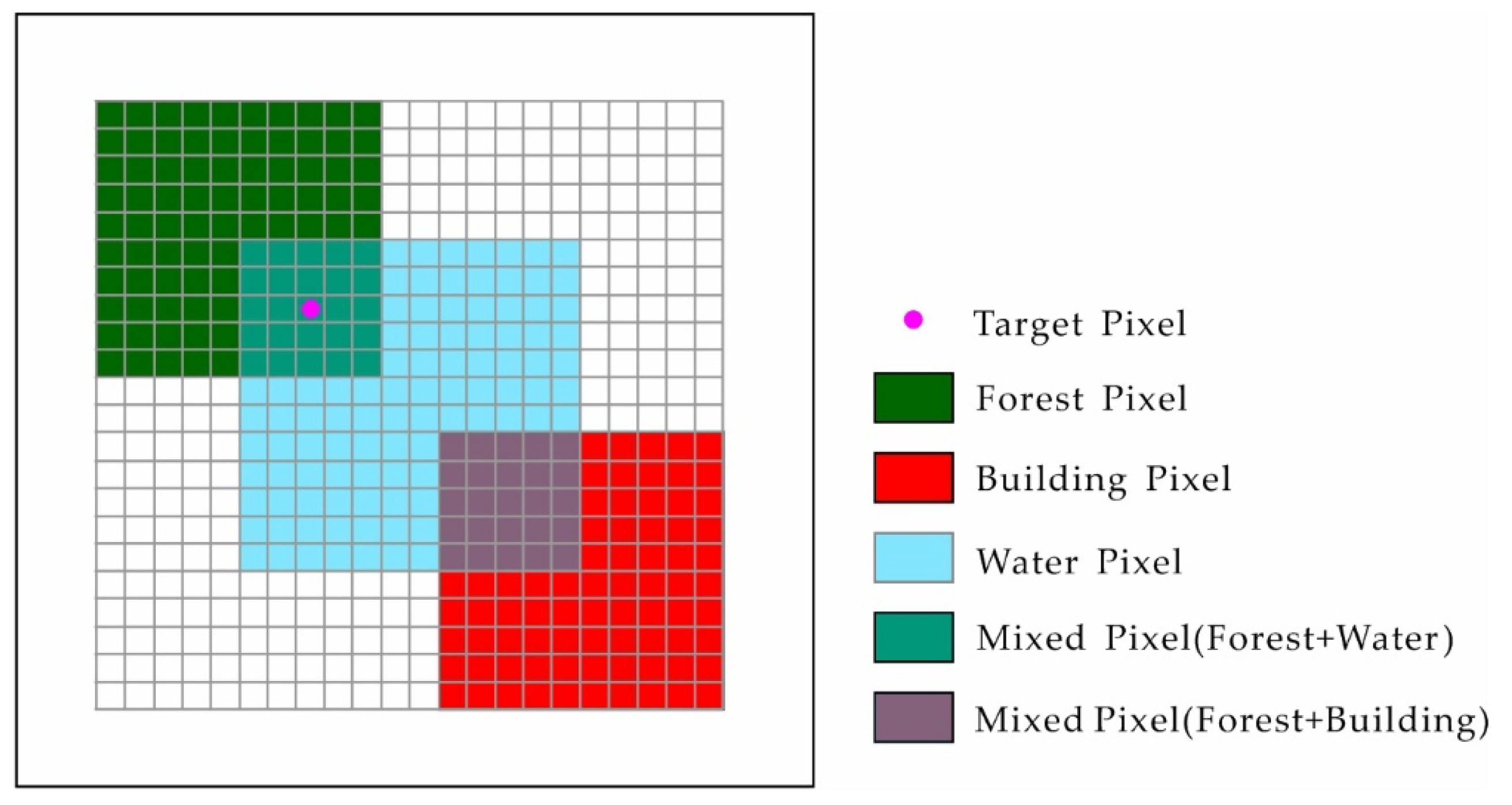
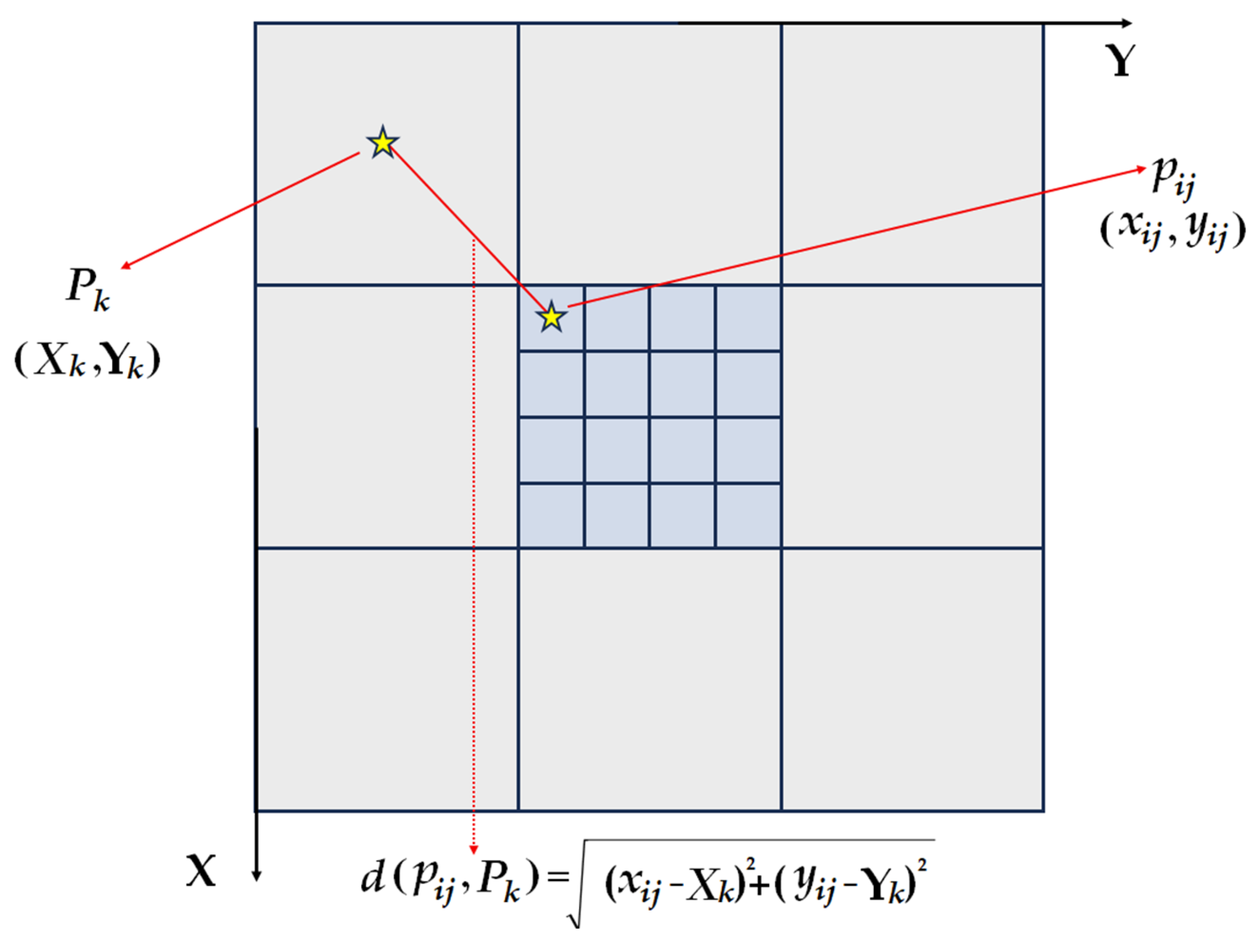
2.5. Sub-Pixel Mapping Based on SPSAM

The mixed pixel decomposition is only able to decompose the proportion of each land class in each pixel, but the specific spatial distribution of classes needs to be solved by further sub-pixel mapping. The principle of sub-pixel mapping is that there is only one type of land class endmember in the sub-pixel obtained after splitting the original pixel by a certain scale factor. The mixed pixel decomposition is carried out on the low-resolution remote sensing image, and then the mixing ratio of each endmember is determined according to the abundance, Finally, the spatial distribution characteristics of each endmember are used to solve the endmember type of each sub-pixel to achieve the sub-pixel-level mapping.

The sub-pixel-pixel spatial attraction model (SPSAM), first proposed by Mertens in 2006, directly calculates the spatial gravity between each sub-pixel and its neighboring low-resolution pixel and classifies the sub-pixels according to their spatial gravity [52,53]. The SPSAM algorithm is based on the following principles: (1) The spatial gravity between the pixels and the sub-pixels is determined by the abundance and distance of the different land classes in the pixels. (2) Sub-pixels in a pixel are only attracted to neighboring pixels. (3) Closer sub-pixels are more attractive than more distant ones, and the gravitational force on sub-pixels from images outside the neighborhood is negligible.

Given that $p_{ij}\left(i,j=1,2,\cdots ,\mathrm{S}\right)$ is a sub-pixel of a certain pixel of the low-resolution image. S is a downscaling factor indicating that each pixel is divided equally into S² sub-pixels (means the spatial resolution is reduced by a factor of S). Then, within its neighboring pixels, there are many neighboring pixels belonging to the mth class of components, i.e., they have similar features or attributes. Thus, the sum of the gravity of the sub-pixels $p_{ij}$ to the mth $\left(\mathrm{m}=1,2,\cdots ,\mathrm{M}\right)$ class of components in its neighboring pixels can be expressed as:

$$D_{m,ij}={\displaystyle \sum }_{k=1}^N{\lambda }_k{F}_m\left(P_k\right)={\displaystyle \sum }_{k=1}^N\frac{F_m\left(P_k\right)}{d_k}$$

(3)

Equation (3) demonstrates that $D_{m,ij}$ denotes the sum of the gravity of the sub−pixel $p_{ij}$ by the mth class component of its neighboring pixels. N denotes the number of neighboringg pixels. $F_m\left(P_k\right)$ denotes the abundance of the kth pixel belonging to the mth class. ${\lambda }_k$ is the spatial correlation weight. As shown in Figure 3, $d_k$ is the Euclidean distance of the center of the sub-pixel from the kth image within the neighboring pixels. In general, ${\lambda }_k$ can be expressed as the reciprocal of $d_k$.

Finally, the sub-pixel belonging to class m within the pixel $p_{ij}$ is determined according to the value of $D_{m,ij}$: If $F_m\left(P_k\right)$ is the component value of class m within $P_{ij}$, then the $F_m\left(P_k\right){\mathrm{S}}^2$ sub-pixels which have the largest gravity value of $D_{m,ij}$ belong to class m.

2.6. Sub-Pixel Mapping Correction Based on Edge-Matching

Although the conventional SPSAM algorithm can divide the pixels into multiple sub-pixels through the gravitational relationship between the pixels, and combine the abundance inversion results to position the distribution situation of forest endmembers. In the whole pixel, this positioning is uncertain due to lack of constraint information. This uncertainty is reflected in that some spatial information on detailed forest edge-distribution is still missing. Some noise pixels present at forest boundaries due to misclassification and omission errors, resulting in a large discrepancy between the outline of the forest and the actual one. To ensure the accuracy of sub-pixel mapping and to further refine the forest cover monitoring results, it is necessary to obtain more information that can constrain the spatial distribution within the mixed pixels. Therefore, it is feasible to extract the forest edge shape from higher resolution images as spatially constrained information for sub-pixel mapping.

In this context, this study proposes an algorithm for sub-pixel mapping correction based on edge-matching, which detects the edge information of pixel by converting the high-resolution image of Jilin-1 into a binarized image and performing edge detection on pixel in the target area. Then, combined with methods such as the Canny operator, the extracted forest edge range can be calculated based on the edge information of pixels. Finally, according to the pixel matching, the sub-pixels positioning is corrected after being sub-pixel mapping in the Sentinel-2.

For complex images such as remote sensing images, image binarization can help to extract the outline of objects in the image, thus helping to extract the edge information more accurately and precisely. As a threshold needs to be determined for image binarization, and considering that the purpose of binarization is to extract forest-wide edges, setting a threshold for a single band will often lose a lot of spectral information. The Jilin-1 image after resampling to 2.5 m (match the downscaling of sentinel-2) needs to be transformed by PCA first, which is a commonly used method for fusion and dimensionality reduction of remote sensing data. Through PCA processing, information from multiple bands can be combined to form a new “principal component” band, thus simplifying the data and extracting information. The forest or non-forested will be divided through the greenness values that are transformed by PCA. When the first principal component load after PCA transformation is the largest and its corresponding greenness value is above 0.25, it can be used as the threshold range for forest. In this study, the greenness threshold is set to 0.25, i.e., other greenness values greater than 0.25 are considered to be forest, and their pixels are assigned to 1, while those less than 0.25 are regarded as non-forest, and their pixels are assigned to 0. The gradient is then calculated by using the Canny operator with the binarized image, and the formula is as follows:

$$G_X=i\left(x+1, y\right)-i\left(x-1, y\right)$$

(4)

$$G_Y=i\left(x, y+1\right)-i\left(x, y-1\right)$$

(5)

Equations (4) and (5) demonstrate that $G_X$ and $G_Y$ represent the gradient intensity of each pixel point in the horizontal and vertical directions, and $i\left(x, y\right)$ represents the input binarised image. The amplitude and direction are then calculated as follows:

$$G=\sqrt{\left(G_X{}^2+G_Y{}^2\right)}$$

(6)

$$\theta =arctan\left(G_Y / G_X\right)$$

(7)

After calculating the magnitude and direction, for each pixel, find two adjacent images in the direction of its gradient and compare their gradient magnitudes, keeping the maximum value and setting the other values to 0. This results in a refined edge image, only the pixel with the largest gradient magnitude is retained, and the possible cases of large edge widths or uncertain orientations are removed, resulting in a more precise edge line.

Double thresholding is the final step in edge detection by the Canny operator. In this step, all pixel points are divided into three categories: strong edges, weak edges, and non-edges. Specifically: (1) pixel points with a gradient amplitude greater than the high threshold T_H are considered “strong edges”; (2) pixel points with a gradient amplitude less than the low threshold T_L are labeled as “non-edge”; and (3) pixel points between the two thresholds are “weak edges”.

For ‘strong edge’ and ‘non-edge’ pixel points, they are output directly to the final image; however, for ‘weak edge’ image points, it is necessary to check whether they are adjacent to a “strong edge” pixel (they can be connected by pixel points in the 8 field). If it can be connected to a ‘strong edge’ pixel point, then it is also marked as a ‘strong edge’ pixel point; otherwise, it is marked as a ‘non-edge’ pixel point. By doing so, a complete edge image can be obtained, including strong edges and some “weak edges”, while most of the noise pixels and non-edge pixels are removed, which has a good edge extraction effect.

Finally, the pixel matching method is used to match the sub-pixel mapping results with the forest edge extracted by Jilin-1. For two binary images with the same number of rows and columns, in the pixel matching, each pixel in the forest edge image is traversed to find the same latitude and longitude pixel in the sub-pixel mapping image, and then its pixel value is assigned to the pixel in the sub-pixel mapping image. This allows for a more accurate spatial distribution of forest edges and helps to reduce noisy pixels due to misclassification and omission error in sub-pixel mapping result. In this way, it is used to complete the sub-pixel mapping with edge-matching correction

2.7. Accuracy Assessment

Accuracy validation is essential in order to evaluate the results of pixel-level forest cover monitoring and sub-pixel-level forest cover monitoring. As shown in

Table 3. Confusion matrix structure of forest cover monitoring.

	Forest in Monitoring	Others in Monitoring
Forest in Real	True Positive (TP)	False Negative (FN)
Other in Real	False Positive (FP)	True Negative (TN)

, a confusion matrix is applied to assess the accuracy of monitoring in this study. It includes four evaluation indicators: overall accuracy, producer accuracy, user accuracy and Kappa coefficient, where OA represents the ratio of the number of correctly monitored pixels to the total number of pixels; PA represents the ratio of the experimentally correctly monitored forest cover area to the total number of pixels indicated for monitoring; UA represents the ratio of the number of real forest cover pixels to the number of experimentally monitored forest cover pixels; and kappa coefficient indicates the consistency between monitoring results and actual results.

The equations for the four evaluation indicators of the confusion matrix are as follows:

(1)

Overall Accuracy (OA):

$$\mathrm{OA}=\frac{TP+TN}{TP+FN+FP+TN}$$

(8)

(2)

Producer Accuracy (PA):

$$\mathrm{PA}=\frac{TP}{TP+FN}$$

(9)

(3)

User Accuracy (UA):

$$\mathrm{UA}=\frac{TP}{TP+FP}$$

(10)

(4)

Kappa coefficient:

$$\mathrm{Kappa}=\frac{OA-P_e}{1-P_e}$$

(11)

Equation (11) demonstrates that $P_e$ represents the probability of model monitoring being correct in a random situation. The formula for $P_e$ can be expressed as

$$P_e=\frac{\left(TP+FN\right)\times \left(TP+FP\right)+\left(FP+TN\right)\times \left(FN+TN\right)}{{(TP+FN+FP+TN)}^2}$$

(12)

In general, the kappa coefficient has an interval range between [0, 1], and in terms of testing for consistency, the kappa coefficient greater than 0.6 can be considered to be substantially consistent, and greater than 0.8 can be considered to be almost perfectly consistent.

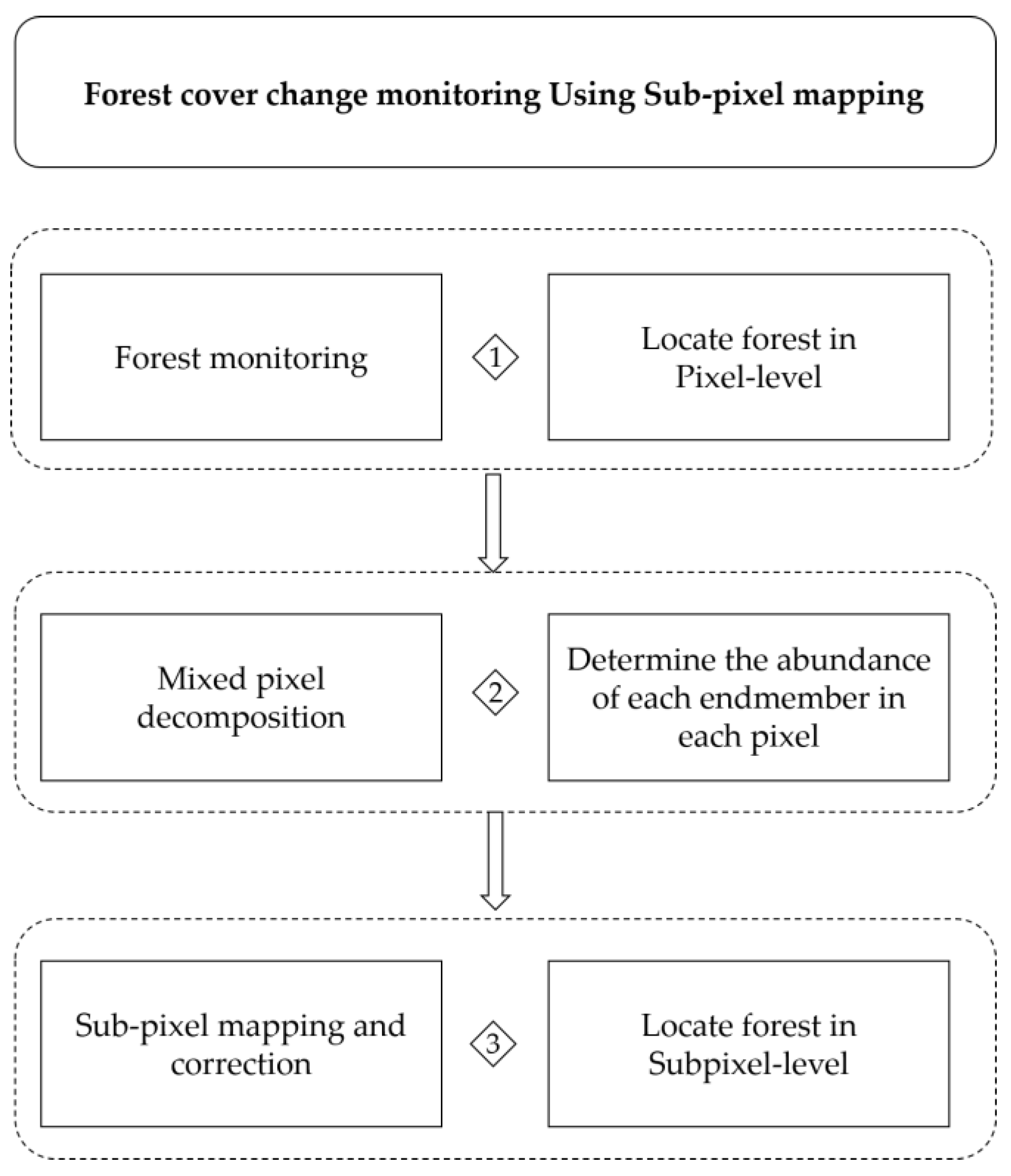
2.8. Graphical Abstract of the Research Program

The Graphical abstract of the research program is shown in Figure 4.

3. Results

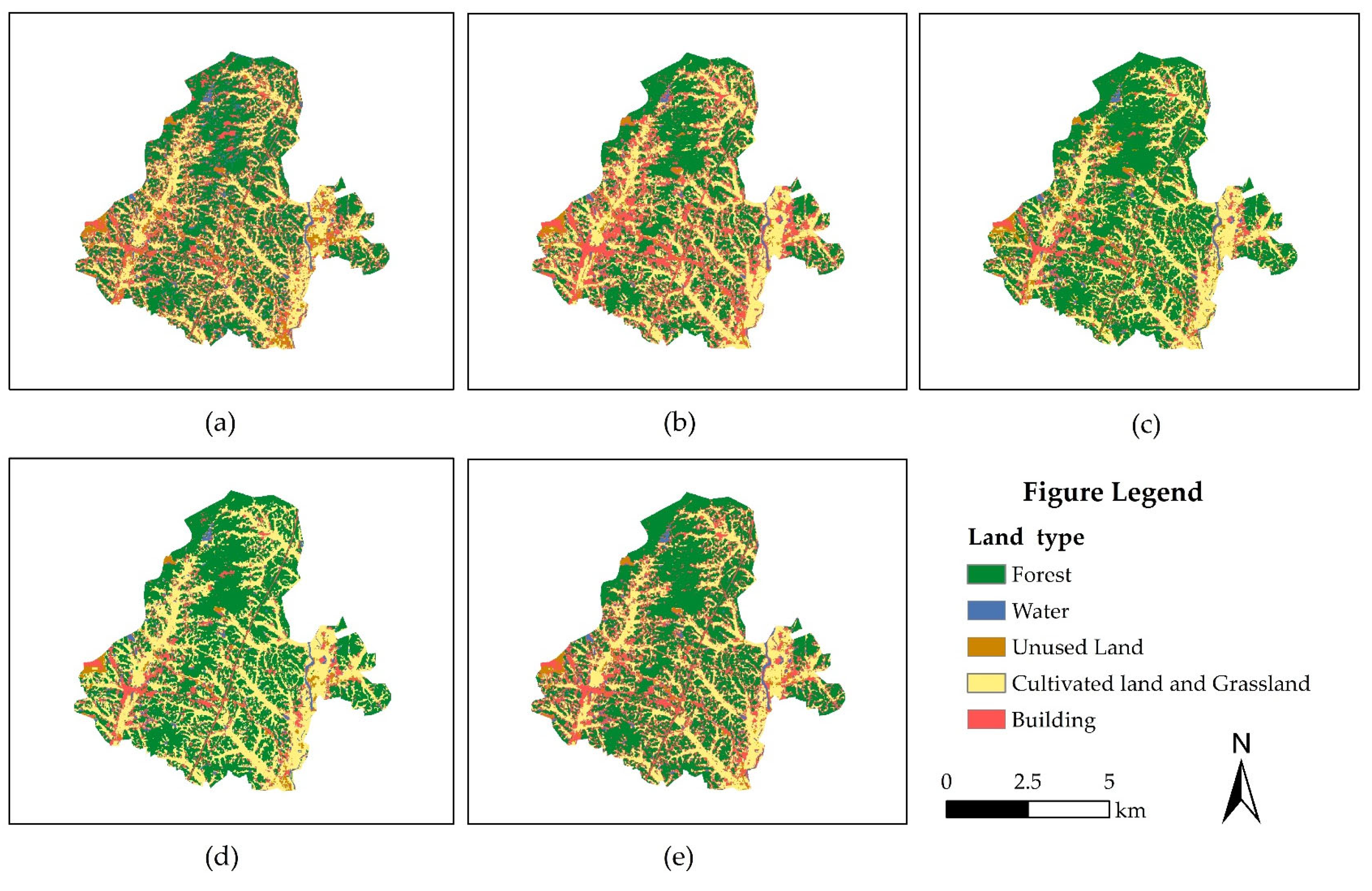
3.1. Result of Pixel-Level Forest Cover Monitoring

Five types of forest monitoring using decision trees, random forests, maximum-likelihood estimation, artificial neural networks, and support vector machines were performed on Sentinel-2 images of the study area on 12 January 2021. Five main land types of forest, water, unused land, cultivated land and grassland, and buildings are selected as samples. As shown in Figure 5, comparing the results of the five pixel-level monitoring methods, the results show that all five pixel-level monitoring methods can classify forest and the remaining major land classes. However, there is still misclassification in forest and other land classes in some areas. The main reason for the misclassification is that these image elements may contain multiple land classes at the same time and are mixed pixels composed of multiple land classes. The types of land classes contained in these pixels may have similar spectral characteristics, making them difficult to distinguish in remote sensing images.

The accuracy of the monitoring results is further rated using the confusion matrix. As shown in

Table 4. Accuracy assessment of pixel-level forest cover monitoring.

Method	OA (%)	Forest PA (%)	Forest UA (%)	Kappa
DT	82.99%	84.34%	81.40%	0.796
MLE	78.07%	76.71%	79.04%	0.732
ANN	80.76%	83.51%	80.05%	0.766
SVM	84.63%	86.14%	83.23%	0.817
RF	87.42%	89.80%	86.69%	0.839

, of the various evaluation metrics in the confusion matrix: overall accuracy refers to the proportion of all pixels that are correctly classified for monitoring. The random forest algorithm performed the best in terms of overall accuracy with 87.42%, while the other algorithms are support vector machine (84.63%), decision tree (82.99%), artificial neural network (80.76%) and maximum-likelihood estimation (78.07%). Forest producer accuracy, which is the classification accuracy for the forest class pixel, is also the best performance of random forest with 89.80%, followed by support vector machine (86.14%), decision tree (84.34%), artificial neural network (83.51%) and maximum-likelihood estimation (76.71%). Forest user accuracy is the proportion of the pixels predicted to be in the forest class that actually belong to that class, and random forests also performed best in this respect with 86.69%, followed by support vector machines (86.14%), decision trees (81.40%), artificial neural networks (80.05%) and maximum- likelihood estimation (79.04%). Finally, the kappa coefficient is a metric that evaluates the overall performance of classification monitoring and takes values ranging from 0 to 1, with higher values indicating that the algorithm is more capable of classification. Random forest is also the best performer in this metric, with a value of 0.839, while the other algorithms are support vector machine (0.817), decision tree (0.796), artificial neural network (0.766) and maximum-likelihood estimation (0.732).

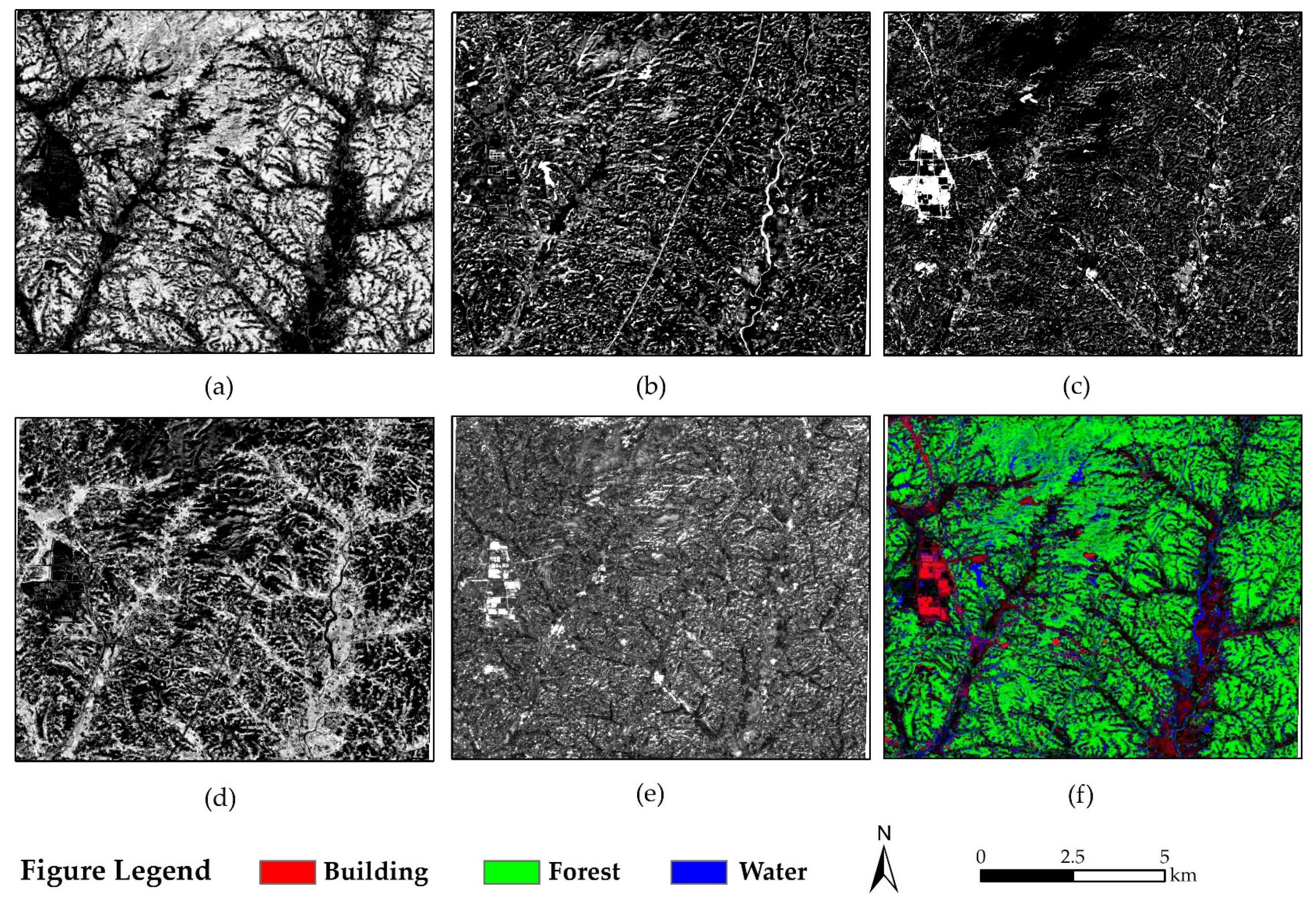
3.2. Results of Mixed-Pixel Decomposition

Based on the pixel-level monitoring results, five endmembers were extracted from the mixed pixel decomposition using fully constrained least squares: forests, waters, unused land, cropland and grassland, and buildings. Figure 6 shows the extracted grey scale map and the retrieval RGB abundance map for each endmember.

Figure 6a shows the abundance of forest endmembers in the form of a greyscale map with pixel values in the range of [0, 1], providing a clear overview of the distribution of forest in the image and the proportion of forest endmembers in the mixed pixel. In this image, the higher the pixel value, the greater the proportion of forest landforms in the pixel, which means that the endmember extraction results are closer to pure forest endmember (the proportion of other land classes in the pixel is almost 0, which is regarded as pure forest endmember). Additionally, Figure 6b–e represent the endmember extraction results for water, unused land, cultivated land and grassland, and building, respectively. Figure 6f shows the abundance result in RGB format.

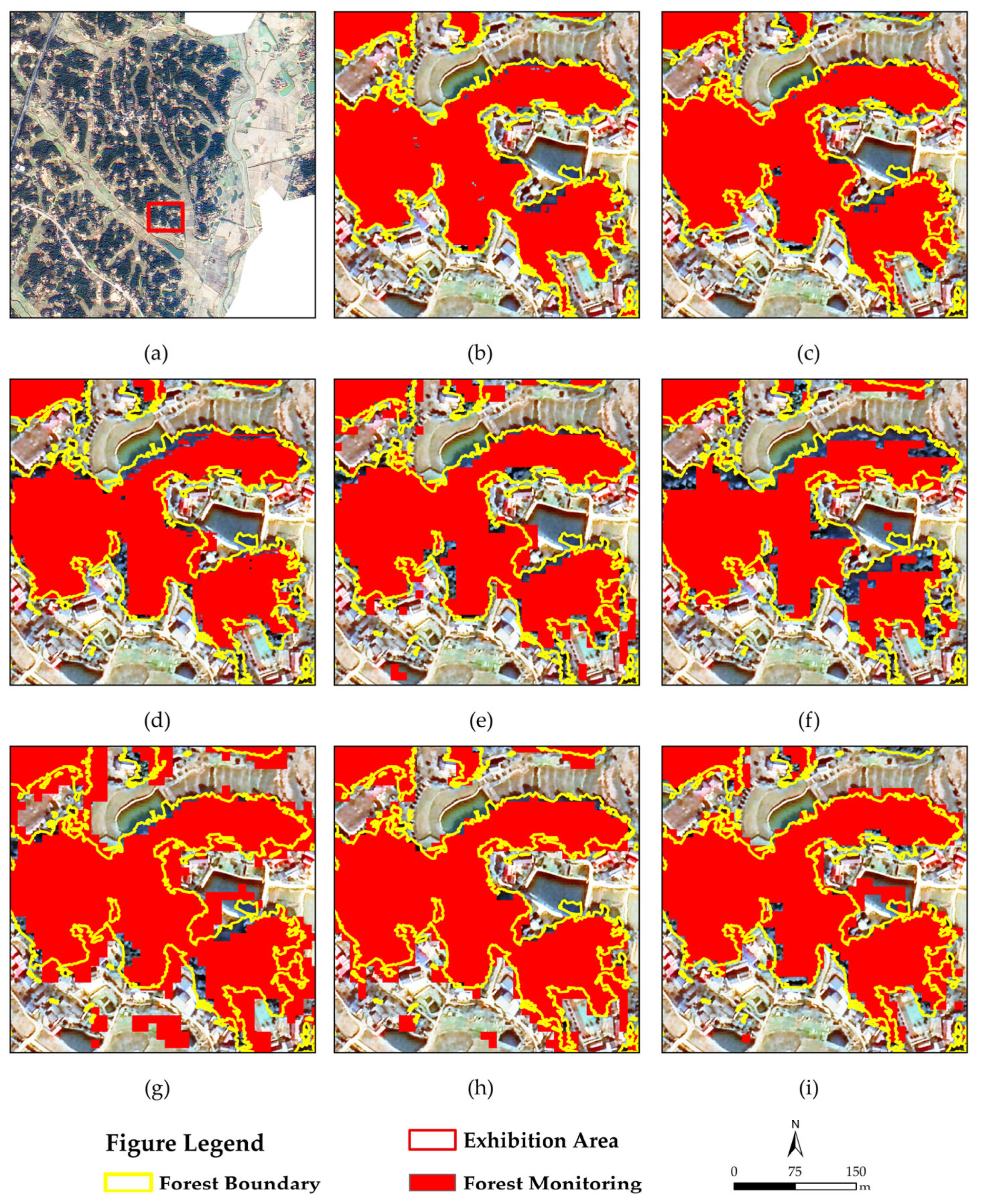
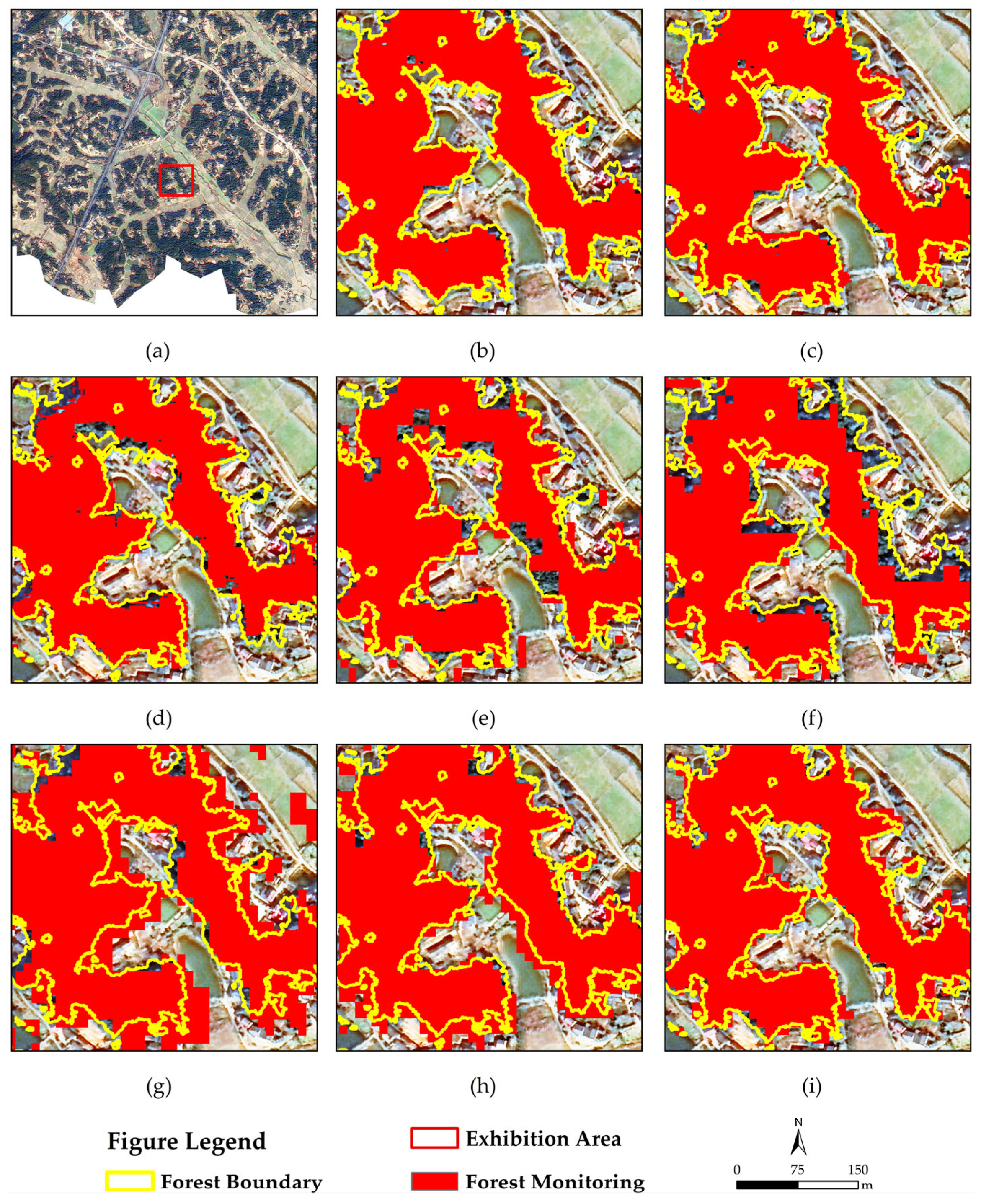
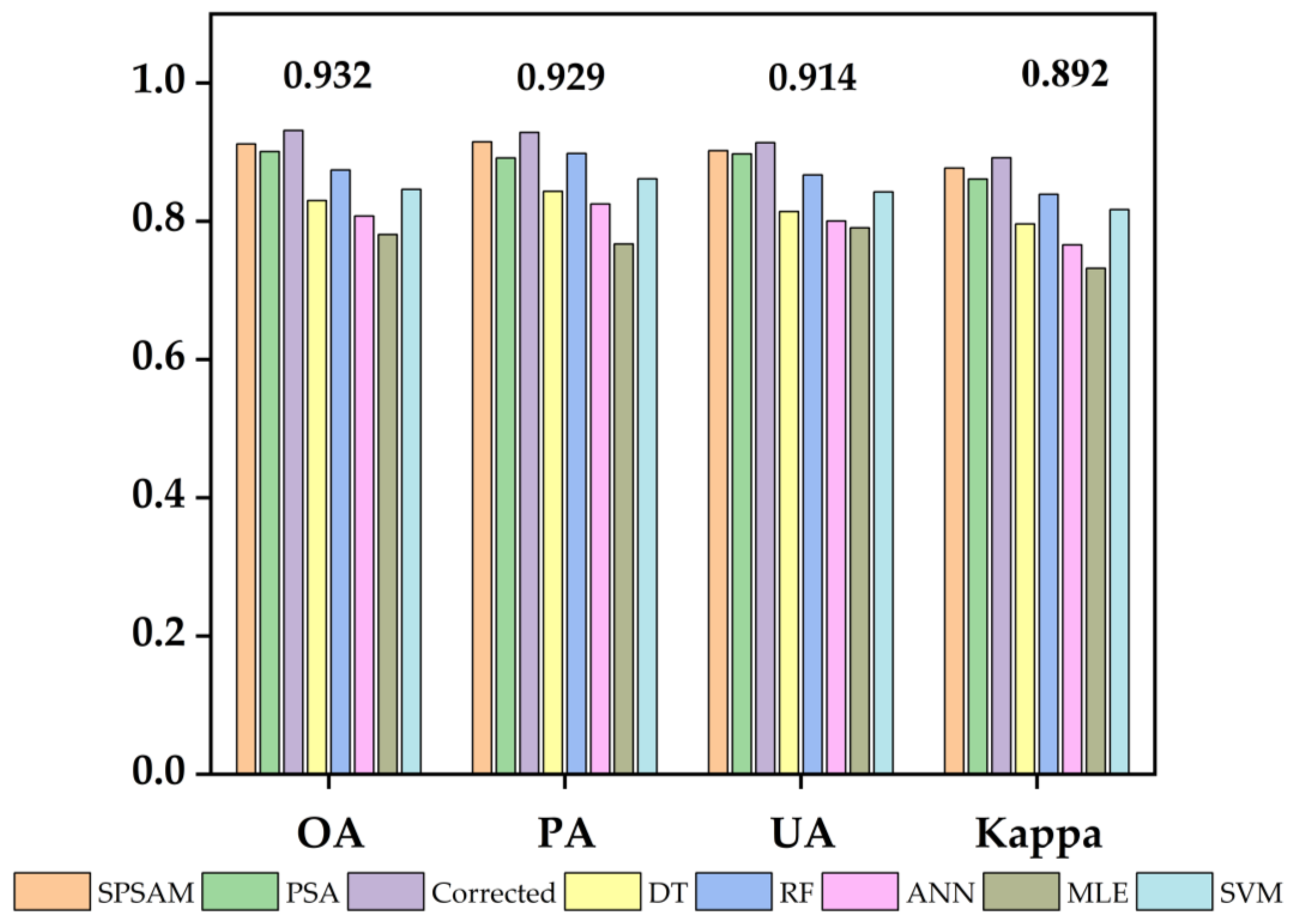
3.3. Results of Sub-Pixel Mapping before and after Correction

To provide a clearer visualization of the results before and after sub-pixel mapping correction, two random rectangles in the image selected as the exhibition area. The comparison was made between these areas and five pixel-level monitoring results, along with the classical sub-pixel mapping method PSA. The corresponding results are shown in Figure 7 and Figure 8.

As shown in Figure 7 and Figure 8, the corrected sub-pixel mapping results are approximately the same as the forest cover range extracted from the Jilin-1 images, while comparing the monitoring results at the pixel-level. The sub-pixel-level monitoring results are less affected by misclassification because the spatial scale is smaller (2.5 m), avoiding the influence of mixed pixels to the greatest extent. The resulting monitoring maps are significantly less noisy than the other algorithms. The pixel-level monitoring results give an approximate picture of the forest cover, but the detail at the boundaries is coarse and difficult to visualize, whereas the sub-pixel-level monitoring results have more spatial detail. Comparing the results of the uncorrected SPSAM model, it can be seen that the spatial information at the forest boundaries is repaired and the forest boundaries are more clearly defined, which makes the mapping of forest cover areas at the sub-pixel-level more accurate and close to the actual forest range. Comparing the results of PSA, it can be clearly observed that PSA has a considerable number of omission at the forest boundary, which is reflected in the obvious shape of the hole. The comparison of the results in the two exhibition areas demonstrates that the sub-pixel mapping with edge-matching correction algorithm, which incorporates edge-matching and optimization techniques, is better able to correct the spatial misalignment of some sub-pixels due to the lack of constraint information in the sub-pixel mapping process. This mapping correction algorithm is more effective than other algorithms for forest cover monitoring.

To better reflect the difference between the sub-pixel mapping results before and after correction, a confusion matrix is used to evaluate the monitoring accuracy in this study. As shown in Figure 9, the orange and purple columns indicate the monitoring accuracy of the sub-pixel mapping result before and after correction, respectively. The results show that the sub-pixel-level monitoring accuracy outperforms the five classification monitoring methods based on pixel-level in all four evaluation metrics.

As shown in

Table 5. Accuracy evaluation of sub-pixel mapping results before and after correction.

Method	OA (%)	Forest PA (%)	Forest UA (%)	Kappa
SPSAM before correction	91.19%	91.48%	90.23%	0.877
SPSAM after correction	93.15%	92.86%	91.37%	0.892

, comparing the accuracy before and after correction, the overall accuracy increases from 91.19% to 93.15% after correction, an improvement of 1.96%. In terms of kappa coefficient, the corrected result is 0.15 higher than the original result, with values of 0.8778 and 0.892, respectively. Both the user accuracy and producer accuracy have improved as well. Although the overall accuracy exceeded 90% before and after correction, the monitoring results image shows that the corrected images have richer spatial information about the location of forest boundaries compared to before correction. These phenomena further demonstrate the superiority of the corrected sub-pixel mapping method. Therefore, it is feasible to use the improved sub-pixel mapping method, which incorporates edge-matching results from Jilin-1 image as constraint information.

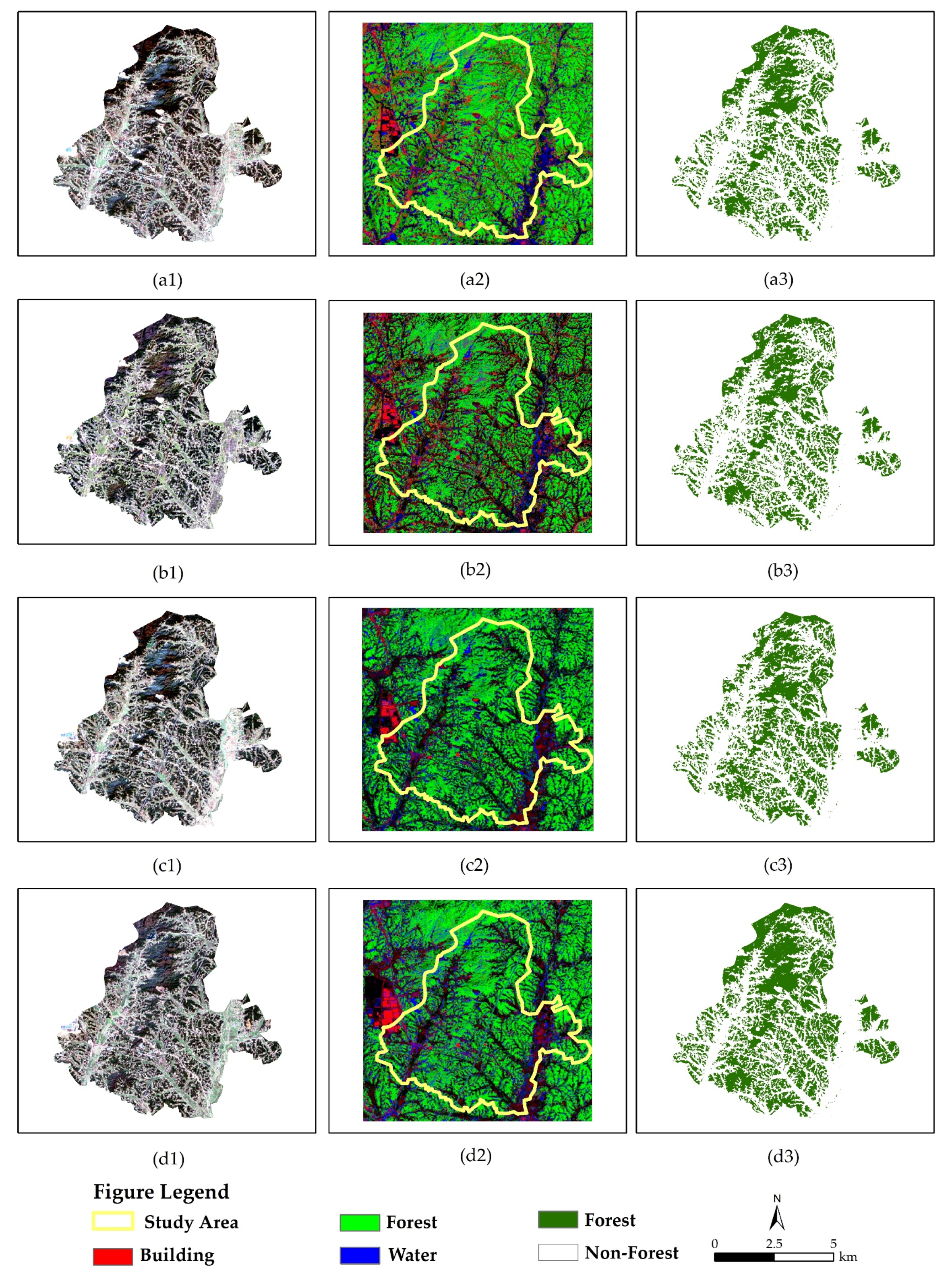
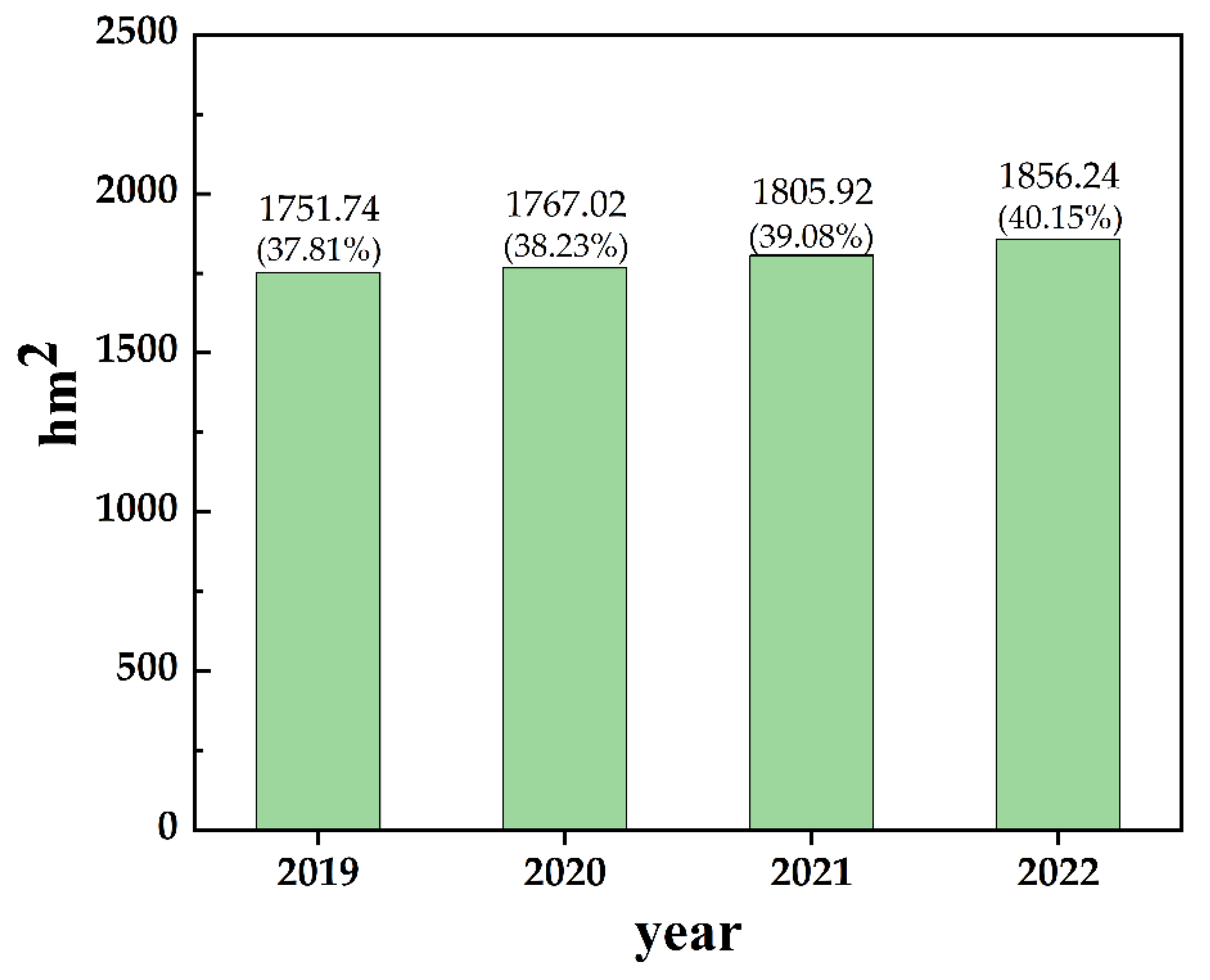
3.4. Sub-Pixel-Level Continuous Monitoring of Forest Cover Change

The corrected SPSAM is used to achieve sub-pixel mapping of forest change in Qingshanpu Town for the four-year period 2019–2022, for which the downscaling factor S is equal to 4. This indicates that a pixel is divided equally into S² = 16 sub-pixels, which corresponds to a downscaling of the spatial resolution by a factor of 4. To ensure the rigor of this study, all four scenes are acquired in January of the current year, and the results are shown in Figure 10.

Based on the monitoring results of forest cover change in Qingshanpu Township during the four-year period from 2019 to 2022, sub-pixel mapping successfully increased the resolution of Sentinel-2 forest cover monitoring to 2.5 m at the sub-pixel-level, and counted the number of sub-pixel of its sub-pixel monitoring results. As shown in Figure 11, the forest cover in Qingshanpu Township has steadily increased in recent years, the proportion of forest has increased from 37.81% in 2019 to 40.15% in 2022. The forest area has increased from 1751.74 hm² in 2019 to 1856.24 hm² in 2022 to 40.15% in 2022, and the area of forest increased from 1751.74 hm² in 2019 to 1856.24 hm² in 2022. This is due to the town’s active promotion of ecological restoration, which has strengthened the construction and protection of forest ecosystems through measures such as afforestation, river management and water source improvement. In addition, the town has strengthened its efforts to combat illegal logging and destruction of forest resources, maintaining the stability and health of the forest ecological environment.

4. Discussion

At present, most of the research on forest cover monitoring is still at the image level and pixel-level, and due to the limitation of its own sensor, there are a large number of mixed pixels in remote sensing images, which makes the refinement of forest cover monitoring greatly limited [54,55]. Sub-pixel mapping technology is mainly applied to the accurate monitoring of land classes in remote sensing images, such as land cover [56,57,58,59], water boundaries [60,61], impermeable surfaces [62,63], etc. It can quantitatively solve the problem of mixed pixels and improve the spatial resolution of monitoring results.

However, there are few studies on sub-pixel mapping for forest cover monitoring. In this study, we selected Qingshanpu Town of Changsha City as the study area, and Sentinel-2 images with a spatial resolution of 10 m as the data source, supplemented with sub-meter Jilin-1 images as the validation data source, A sub-pixel mapping correction algorithm using edge-matching is proposed, followed by a discussion of the results.

In mixed pixel decomposition, the linear spectral mixing model is considered to be a more effective model for solving mixed pixels and is therefore widely used in spectral unmixing [64,65]. In this study, the linear spectral unmixing of five land classes identified in the pixel-level monitoring is performed as five endmembers, and this method completed the abundance inversion to determine the abundance of endmembers in the mixed pixels. The abundance result reflects the percentage of different land classes in the pixels.

However, mixed pixel decomposition can only determine the abundance of each class of endmembers in the pixel, and does not accurately represent the spatial distribution within it. Through sub-pixel mapping techniques, mixed pixels can be accurately decomposed to the sub-pixel-level, and the spatial layout of forest within the pixel can be more accurately estimated, and forest cover change can be monitored at a smaller scale. SPSAM models are used in sub-pixel mapping due to the lack of constraint information. However, conventional SPSAM models still perform poorly at the edges where forest and other classes converge, lacking information on boundary details and causing some pixel misclassification and omission. There are some circumventions of pixel misclassification and omission being proposed by methods previous studies, such as the introduction of additional auxiliary information constraints [66,67]. In this study, the forest boundary is extracted from the higher resolution Jilin-1 image by an edge-matching algorithm, and the misclassification or omission pixels are corrected by pixel matching to address the lack of refinement of image monitoring due to the loss of forest boundary detail information. The accuracy of the corrected results is improved compared to the pixel-level monitoring, with an overall accuracy of 93.15%. The contour details of the forest boundaries are also closer to the actual situation.

Continuous dynamic monitoring of forest cover change in the Qingshanpu Town area over time, achieved through corrected sub-pixel mapping, has been found to be feasible with the Sentinel-2 data used in this study. The sub-pixel-level forest cover monitoring resolution is successfully downscaled to 2.5 m, further refining the accuracy of forest cover monitoring. This improved monitoring method provides valuable scientific information for forest resource management. Sub-pixel-level monitoring of forest cover change can effectively address the problem of monitoring errors caused by inadequate spatial resolution of images captured by sensors.

One of the limitations of this study is the restricted temporal resolution of both Senti-nel-2 and Jilin-1 images, which hinders the ability to generate long time series of forest cover monitoring. In future research, the combination of multi-source remote sensing image should be considered to try out long time series of sub-pixel-level forest cover monitoring research. Additionally, the methodology of this study may also be able to be applied to the monitoring of small-scale changes in forests caused by deforestation, pests and diseases, or forest fires, which will be one of the subsequent studies.

5. Conclusions

Remote sensing technology is an important tool for forest cover monitoring. In this study, five traditional classifiers, DT, MLE, ANN, SVN and RE, are used to monitor the forest cover at pixel-level in the study area and to analyze the accuracy of pixel-level monitoring. The results show that random forest has the highest accuracy in pixel-level monitoring, with OA reaching 87.42%, PA reaching 88.80%, UA reaching 86.69% and kappa coefficient of 0.839, which are the highest in all four indicators. However, due to the influence of mixed pixels, there are still misclassification or omission of forest and other land classes in some areas, particularly at the junction of forest and other land classes, significantly limiting the accuracy of pixel-level monitoring. Based on the SPSAM sub-pixel mapping model, this study partitions the pixels into 16 refined sub-pixels according to the downscaling factor through the gravitational relationship between pixels and sub-pixels and assigns the spatial information of the land classes to the sub-pixels according to the abundance inversion results. This method has successfully achieved sub-pixel-level extraction of forest cover in the study area by downscaling the spatial resolution of forest monitoring results to 2.5 m, thus surpassing the 10 m limit of Sentinel-2 image’s spatial resolution. Subsequently, a combination of sub-meter resolution Jilin-1 image and a sub-pixel mapping correction algorithm using edge-matching is employed to correct the edge outline details of the sub-pixel forest monitoring results to bring the forest extent closer to the actual results. The results show that the sub-pixel-level monitoring accuracy outperforms the five classification-based monitoring methods at the pixel-level in all four evaluation metrics. Comparing the results of another subpixel mapping PSA, the corrected SPSAM exhibits smoother at the forest boundary, Additionally, the shape of the holes at the boundary is significantly improved. Evaluating the SPSAM accuracy before and after correction, the overall accuracy increased from 91.19% to 93.15%, representing an improvement of 1.96% compared to the uncorrected results. In terms of kappa coefficient, the corrected results improved by 0.15 compared to the original result, with values of 0.877 and 0.892, respectively. Both the user accuracy and producer accuracy have also improved. The corrected results have richer spatial information at the forest boundary positions than before the correction.

The corrected SPSAM model is used to monitor forest cover changes at the sub-pixel-level for four years from 2019 to 2022 in Qingshanpu Town. The results show that the forest cover in Qingshanpu Town has steadily increased in recent years, with the proportion of forest increasing from 37.81% in 2019 to 40.15% in 2022, and the area of forested land increasing from 1751.74 hm² in 2019 to 1856.24 hm² in 2022. In conclusion, forest cover monitoring at the sub-pixel-level can more accurately assess forest cover changes, improve forest management efficiency and provide new references for forestry resource management.

References

1. Mononen, L.; Auvinen, A.-P.; Ahokumpu, A.-L.; Rönkä, M.; Aarras, N.; Tolvanen, H.; Kamppinen, M.; Viirret, E.; Kumpula, T.; Vihervaara, P. National Ecosystem Service Indicators: Measures of Social–Ecological Sustainability. Ecol. Indic. 2016, 61, 27–37. [Google Scholar] [CrossRef]
2. Nesha, K.; Herold, M.; De Sy, V.; Duchelle, A.E.; Martius, C.; Branthomme, A.; Garzuglia, M.; Jonsson, O.; Pekkarinen, A. An Assessment of Data Sources, Data Quality and Changes in National Forest Monitoring Capacities in the Global Forest Resources Assessment 2005–2020. Environ. Res. Lett. 2021, 16, 054029. [Google Scholar] [CrossRef]
3. He, Y.; Jia, K.; Wei, Z. Improvements in Forest Segmentation Accuracy Using a New Deep Learning Architecture and Data Augmentation Technique. Remote Sens. 2023, 15, 2412. [Google Scholar] [CrossRef]
4. Loranty, M.; Davydov, S.; Kropp, H.; Alexander, H.; Mack, M.; Natali, S.; Zimov, N. Vegetation Indices Do Not Capture Forest Cover Variation in Upland Siberian Larch Forests. Remote Sens. 2018, 10, 1686. [Google Scholar] [CrossRef]
5. Tlig, L.; Bouchouicha, M.; Tlig, M.; Sayadi, M.; Moreau, E. A Fast Segmentation Method for Fire Forest Images Based on Multiscale Transform and PCA. Sensors 2020, 20, 6429. [Google Scholar] [CrossRef] [PubMed]
6. Beguet, B.; Chehata, N.; Boukir, S.; Guyon, D. Classification of Forest Structure Using Very High Resolution Pleiades Image Texture. In Proceedings of the 2014 IEEE Geoscience and Remote Sensing Symposium, Quebec City, QC, Canada, 13–18 July 2014; pp. 2324–2327. [Google Scholar]
7. Chehata, N.; Orny, C.; Boukir, S.; Guyon, D. Object-Based Forest Change Detection Using High Resolution Satellite Images. Int. Arch. Photogramm. Remote Sens. Spat. Inf. Sci. 2013, 38, 49–54. [Google Scholar] [CrossRef]
8. Heckel, K.; Urban, M.; Schratz, P.; Mahecha, M.; Schmullius, C. Predicting Forest Cover in Distinct Ecosystems: The Potential of Multi-Source Sentinel-1 and -2 Data Fusion. Remote Sens. 2020, 12, 302. [Google Scholar] [CrossRef]
9. Liang, J.; Ren, C.; Li, Y.; Yue, W.; Wei, Z.; Song, X.; Zhang, X.; Yin, A.; Lin, X. Using Enhanced Gap-Filling and Whittaker Smoothing to Reconstruct High Spatiotemporal Resolution NDVI Time Series Based on Landsat 8, Sentinel-2, and MODIS Imagery. ISPRS Int. J. Geo-Inf. 2023, 12, 214. [Google Scholar] [CrossRef]
10. Matsushita, B.; Yang, W.; Chen, J.; Onda, Y.; Qiu, G. Sensitivity of the Enhanced Vegetation Index (EVI) and Normalized Difference Vegetation Index (NDVI) to Topographic Effects: A Case Study in High-Density Cypress Forest. Sensors 2007, 7, 2636–2651. [Google Scholar] [CrossRef]
11. Xue, J.; Su, B. Significant Remote Sensing Vegetation Indices: A Review of Developments and Applications. J. Sens. 2017, 2017, 1353691. [Google Scholar] [CrossRef]
12. Zhu, Y.; Yao, X.; Tian, Y.; Liu, X.; Cao, W. Analysis of Common Canopy Vegetation Indices for Indicating Leaf Nitrogen Accumulations in Wheat and Rice. Int. J. Appl. Earth Obs. Geoinf. 2008, 10, 1–10. [Google Scholar] [CrossRef]
13. Coladello, L.F.; de Lourdes Bueno Trindade Galo, M.; Shimabukuro, M.H.; Ivánová, I.; Awange, J. Macrophytes’ Abundance Changes in Eutrophicated Tropical Reservoirs Exemplified by Salto Grande (Brazil): Trends and Temporal Analysis Exploiting Landsat Remotely Sensed Data. Appl. Geogr. 2020, 121, 102242. [Google Scholar] [CrossRef]
14. Al-Ani, L.A.A.; Al-Taei, M.S.M. Multi-Band Image Classification Using Klt and Fractal Classifier. J. Al-Nahrain Univ. Sci. 2011, 14, 171–178. [Google Scholar] [CrossRef]
15. Rahman, S.; Mesev, V. Change Vector Analysis, Tasseled Cap, and NDVI-NDMI for Measuring Land Use/Cover Changes Caused by a Sudden Short-Term Severe Drought: 2011 Texas Event. Remote Sens. 2019, 11, 2217. [Google Scholar] [CrossRef]
16. Franklin, S.E.; Hall, R.J.; Moskal, L.M.; Maudie, A.J.; Lavigne, M.B. Incorporating Texture into Classification of Forest Species Composition from Airborne Multispectral Images. Int. J. Remote Sens. 2000, 21, 61–79. [Google Scholar] [CrossRef]
17. Zawadzki, J.; Cieszewski, C.; Zasada, M.; Lowe, R. Applying Geostatistics for Investigations of Forest Ecosystems Using Remote Sensing Imagery. Silva Fenn. 2005, 39, 599. [Google Scholar] [CrossRef]
18. Gibson, R.K.; Mitchell, A.; Chang, H.-C. Image Texture Analysis Enhances Classification of Fire Extent and Severity Using Sentinel 1 and 2 Satellite Imagery. Remote Sens. 2023, 15, 3512. [Google Scholar] [CrossRef]
19. Wang, Z.; Wei, C.; Liu, X.; Zhu, L.; Yang, Q.; Wang, Q.; Zhang, Q.; Meng, Y. Object-Based Change Detection for Vegetation Disturbance and Recovery Using Landsat Time Series. GISci. Remote Sens. 2022, 59, 1706–1721. [Google Scholar] [CrossRef]
20. Maxwell, A.E.; Warner, T.A.; Fang, F. Implementation of Machine-Learning Classification in Remote Sensing: An Applied Review. Int. J. Remote Sens. 2018, 39, 2784–2817. [Google Scholar] [CrossRef]
21. Brovelli, M.A.; Sun, Y.; Yordanov, V. Monitoring Forest Change in the Amazon Using Multi-Temporal Remote Sensing Data and Machine Learning Classification on Google Earth Engine. ISPRS Int. J. Geo-Inf. 2020, 9, 580. [Google Scholar] [CrossRef]
22. Yao, B.; Zhang, H.Q.; Liu, Y.; Liu, H.; Ling, C.S. Remote Sensing Classification of Wetlands based on Object-oriented and CART Decision Tree Method. For. Res. 2019, 32, 91–98. [Google Scholar] [CrossRef]
23. Sisodia, P.S.; Tiwari, V. Analysis of Supervised Maximum Likelihood Classification for Remote Sensing Image. In Proceedings of the International Conference on Recent Advances and Innovations in Engineering (ICRAIE-2014), Jaipur, India, 9–11 May 2014; pp. 1–4. [Google Scholar] [CrossRef]
24. Dahiya, N.; Singh, S.; Gupta, S.; Rajab, A.; Hamdi, M.; Elmagzoub, M.; Sulaiman, A.; Shaikh, A. Detection of Multitemporal Changes with Artificial Neural Network-Based Change Detection Algorithm Using Hyperspectral Dataset. Remote Sens. 2023, 15, 1326. [Google Scholar] [CrossRef]
25. Bazi, Y.; Melgani, F. Toward an Optimal SVM Classification System for Hyperspectral Remote Sensing Images. IEEE Trans. Geosci. Remote Sens. 2006, 44, 3374–3385. [Google Scholar] [CrossRef]
26. Wang, X.; Gao, X.; Zhang, Y.; Fei, X.; Chen, Z.; Wang, J.; Zhang, Y.; Lu, X.; Zhao, H. Land-Cover Classification of Coastal Wetlands Using the RF Algorithm for Worldview-2 and Landsat 8 Images. Remote Sens. 2019, 11, 1927. [Google Scholar] [CrossRef]
27. Feng, S.; Fan, F. Analyzing the Effect of the Spectral Interference of Mixed Pixels Using Hyperspectral Imagery. IEEE J. Sel. Top. Appl. Earth Obs. Remote Sens. 2021, 14, 1434–1446. [Google Scholar] [CrossRef]
28. Xu, X.; Tong, X.; Plaza, A.; Li, J.; Zhong, Y.; Xie, H.; Zhang, L. A New Spectral-Spatial Sub-Pixel Mapping Model for Remotely Sensed Hyperspectral Imagery. IEEE Trans. Geosci. Remote Sens. 2018, 56, 6763–6778. [Google Scholar] [CrossRef]
29. Su, L.; Xu, Y.; Yuan, Y.; Yang, J. Combining Pixel Swapping and Simulated Annealing for Land Cover Mapping. Sensors 2020, 20, 1503. [Google Scholar] [CrossRef]
30. Mertens, K.C.; de Baets, B.; Verbeke, L.P.C.; de Wulf, R.R. A Sub-pixel Mapping Algorithm Based on Sub-pixel/Pixel Spatial Attraction Models. Int. J. Remote Sens. 2006, 27, 3293–3310. [Google Scholar] [CrossRef]
31. Kasetkasem, T.; Rakwatin, P.; Sirisommai, R.; Eiumnoh, A. A Joint Land Cover Mapping and Image Registration Algorithm Based on a Markov Random Field Model. Remote Sens. 2013, 5, 5089–5121. [Google Scholar] [CrossRef]
32. He, D.; Zhong, Y.; Feng, R.; Zhang, L. Spatial-Temporal Sub-Pixel Mapping Based on Swarm Intelligence Theory. Remote Sens. 2016, 8, 894. [Google Scholar] [CrossRef]
33. Liu, C.; Shi, J.; Liu, X.; Shi, Z.; Zhu, J. Subpixel Mapping of Surface Water in the Tibetan Plateau with MODIS Data. Remote Sens. 2020, 12, 1154. [Google Scholar] [CrossRef]
34. Hu, D.; Chen, S.; Qiao, K.; Cao, S. Integrating CART Algorithm and Multi-Source Remote Sensing Data to Estimate Sub-Pixel Impervious Surface Coverage: A Case Study from Beijing Municipality, China. Chin. Geogr. Sci. 2017, 27, 614–625. [Google Scholar] [CrossRef]
35. Wickramasinghe, C.; Jones, S.; Reinke, K.; Wallace, L. Development of a Multi-Spatial Resolution Approach to the Surveillance of Active Fire Lines Using Himawari-8. Remote Sens. 2016, 8, 932. [Google Scholar] [CrossRef]
36. Ruescas, A.B.; Sobrino, J.A.; Julien, Y.; Jiménez-Muñoz, J.C.; Sòria, G.; Hidalgo, V.; Atitar, M.; Franch, B.; Cuenca, J.; Mattar, C. Mapping Sub-Pixel Burnt Percentage Using AVHRR Data. Application to the Alcalaten Area in Spain. Int. J. Remote Sens. 2010, 31, 5315–5330. [Google Scholar] [CrossRef]
37. Grivei, A.-C.; Vaduva, C.; Datcu, M. Assessment of Burned Area Mapping Methods for Smoke Covered Sentinel-2 Data. In Proceedings of the 2020 13th International Conference on Communications (COMM), Bucharest, Romania, 18–20 June 2020; pp. 189–192. [Google Scholar]
38. Jiang, L.; Zhou, C.; Li, X. Sub-Pixel Surface Water Mapping for Heterogeneous Areas from Sentinel-2 Images: A Case Study in the Jinshui Basin, China. Water 2023, 15, 1446. [Google Scholar] [CrossRef]
39. Li, L.; Chen, Y.; Xu, T.; Shi, K.; Liu, R.; Huang, C.; Lu, B.; Meng, L. Remote Sensing of Wetland Flooding at a Sub-Pixel Scale Based on Random Forests and Spatial Attraction Models. Remote Sens. 2019, 11, 1231. [Google Scholar] [CrossRef]
40. Chen, Y.; Ge, Y.; An, R.; Chen, Y. Super-Resolution Mapping of Impervious Surfaces from Remotely Sensed Imagery with Points-of-Interest. Remote Sens. 2018, 10, 242. [Google Scholar] [CrossRef]
41. Xu, H.; Zhang, G.; Zhou, Z.; Zhou, X.; Zhou, C. Forest Fire Monitoring and Positioning Improvement at Subpixel Level: Application to Himawari-8 Fire Products. Remote Sens. 2022, 14, 2460. [Google Scholar] [CrossRef]
42. Xu, H.; Zhang, G.; Zhou, Z.; Zhou, X.; Zhang, J.; Zhou, C. Development of a Novel Burned-Area Subpixel Mapping (BASM) Workflow for Fire Scar Detection at Subpixel Level. Remote Sens. 2022, 14, 3546. [Google Scholar] [CrossRef]
43. Li, X.; Zhang, G.; Tan, S.; Yang, Z.; Wu, X. Forest Fire Smoke Detection Research Based on the Random Forest Algorithm and Sub-Pixel Mapping Method. Forests 2023, 14, 485. [Google Scholar] [CrossRef]
44. Song, T.; Tang, B.; Zhao, M.; Deng, L. An Accurate 3-D Fire Location Method Based on Sub-Pixel Edge Detection and Non-Parametric Stereo Matching. Measurement 2014, 50, 160–171. [Google Scholar] [CrossRef]
45. Kupfer, B.; Netanyahu, N.S.; Shimshoni, I. An Efficient SIFT-Based Mode-Seeking Algorithm for Sub-Pixel Registration of Remotely Sensed Images. IEEE Geosci. Remote Sens. Lett. 2015, 12, 379–383. [Google Scholar] [CrossRef]
46. Zhang, J.; Wang, Z.; Yang, C.; Ye, S.H. Sub-Pixel Edge Estimation Based on Matching Template. In Proceedings of the International Conference of Optical Instrument and Technology, Beijing, China, 16–19 November 2008; SPIE: Bellingham, WA, USA, 2008; p. 71602A. [Google Scholar]
47. Nghiyalwa, H.S.; Urban, M.; Baade, J.; Smit, I.P.J.; Ramoelo, A.; Mogonong, B.; Schmullius, C. Spatio-Temporal Mixed Pixel Analysis of Savanna Ecosystems: A Review. Remote Sens. 2021, 13, 3870. [Google Scholar] [CrossRef]
48. Yin, C.L.; Meng, F.; Yu, Q.R. Calculation of Land Surface Emissivity and Retrieval of Land Surface Temperature Based on a Spectral Mixing Model. Infrared Phys. Technol. 2020, 108, 103333. [Google Scholar] [CrossRef]
49. Belgiu, M.; Stein, A. Spatiotemporal Image Fusion in Remote Sensing. Remote Sens. 2019, 11, 818. [Google Scholar] [CrossRef]
50. Jones, J. Improved Automated Detection of Subpixel-Scale Inundation—Revised Dynamic Surface Water Extent (DSWE) Partial Surface Water Tests. Remote Sens. 2019, 11, 374. [Google Scholar] [CrossRef]
51. Heinz, D.C.; Chang, C.-I. Fully Constrained Least Squares Linear Spectral Mixture Analysis Method for Material Quantification in Hyperspectral Imagery. IEEE Trans. Geosci. Remote Sens. 2001, 39, 529–545. [Google Scholar] [CrossRef]
52. Wang, Q.; Wang, L.; Liu, D. Integration of Spatial Attractions between and within Pixels for Sub-Pixel Mapping. J. Syst. Eng. Electron. 2012, 23, 293–303. [Google Scholar] [CrossRef]
53. Zhao, C.; Yang, H.; Zhu, H.; Yan, Y. Sub-Pixel Mapping of Remote Sensing Images Based on Sub-Pixel/Pixel Spatial Attraction Models with Anisotropic Spatial Dependence Model. In Proceedings of the 2017 First International Conference on Electronics Instrumentation & Information Systems (EIIS), Harbin, China, 3–5 June 2017; pp. 1–5. [Google Scholar]
54. Bijeesh, T.V.; Narasimhamurthy, K.N. Surface Water Detection and Delineation Using Remote Sensing Images: A Review of Methods and Algorithms. Sustain. Water Resour. Manag. 2020, 6, 68. [Google Scholar] [CrossRef]
55. Kaur, S.; Bansal, R.K.; Mittal, M.; Goyal, L.M.; Kaur, I.; Verma, A.; Son, L.H. Mixed Pixel Decomposition Based on Extended Fuzzy Clustering for Single Spectral Value Remote Sensing Images. J. Indian Soc. Remote Sens. 2019, 47, 427–437. [Google Scholar] [CrossRef]
56. Wang, Q.; Ding, X.; Tong, X.; Atkinson, P.M. Spatio-Temporal Spectral Unmixing of Time-Series Images. Remote Sens. Environ. 2021, 259, 112407. [Google Scholar] [CrossRef]
57. Msellmi, B.; Picone, D.; Ben Rabah, Z.; Dalla Mura, M.; Farah, I.R. Sub-Pixel Mapping Model Based on Total Variation Regularization and Learned Spatial Dictionary. Remote Sens. 2021, 13, 190. [Google Scholar] [CrossRef]
58. Li, X.; Chen, R.; Foody, G.M.; Wang, L.; Yang, X.; Du, Y.; Ling, F. Spatio-Temporal Sub-Pixel Land Cover Mapping of Remote Sensing Imagery Using Spatial Distribution Information From Same-Class Pixels. Remote Sens. 2020, 12, 503. [Google Scholar] [CrossRef]
59. He, D.; Zhong, Y.; Zhang, L. Spectral–Spatial–Temporal MAP-Based Sub-Pixel Mapping for Land-Cover Change Detection. IEEE Trans. Geosci. Remote Sens. 2020, 58, 1696–1717. [Google Scholar] [CrossRef]
60. Wang, X.; Ling, F.; Yao, H.; Liu, Y.; Xu, S. Unsupervised Sub-Pixel Water Body Mapping with Sentinel-3 OLCI Image. Remote Sens. 2019, 11, 327. [Google Scholar] [CrossRef]
61. Liu, Q.; Trinder, J.; Turner, I. A comparison of sub-pixel mapping methods for coastal areas. ISPRS Ann. Photogramm. Remote Sens. Spat. Inf. Sci. 2016, III-7, 67–74. [Google Scholar] [CrossRef]
62. Panigrahi, N.; Tiwari, A.; Dixit, A. Image Pan-Sharpening and Sub-Pixel Classification Enabled Building Detection in Strategically Challenged Forest Neighborhood Environment. J. Indian Soc. Remote Sens. 2021, 49, 2113–2123. [Google Scholar] [CrossRef]
63. Patidar, N.; Keshari, A.K. A Rule-Based Spectral Unmixing Algorithm for Extracting Annual Time Series of Sub-Pixel Impervious Surface Fraction. Int. J. Remote Sens. 2020, 41, 3970–3992. [Google Scholar] [CrossRef]
64. Taureau, F.; Robin, M.; Proisy, C.; Fromard, F.; Imbert, D.; Debaine, F. Mapping the Mangrove Forest Canopy Using Spectral Unmixing of Very High Spatial Resolution Satellite Images. Remote Sens. 2019, 11, 367. [Google Scholar] [CrossRef]
65. Cavalli, R.M. Spatial Validation of Spectral Unmixing Results: A Case Study of Venice City. Remote Sens. 2022, 14, 5165. [Google Scholar] [CrossRef]
66. Ling, F.; Li, X.; Xiao, F.; Fang, S.; Du, Y. Object-Based Sub-Pixel Mapping of Buildings Incorporating the Prior Shape Information from Remotely Sensed Imagery. Int. J. Appl. Earth Obs. Geoinf. 2012, 18, 283–292. [Google Scholar] [CrossRef]
67. Wang, Q.; Zhang, C.; Atkinson, P.M. Sub-Pixel Mapping with Point Constraints. Remote Sens. Environ. 2020, 244, 111817. [Google Scholar] [CrossRef]
Figure 1. Geographical location map of the study areas.
Forests 14 01776 g001
Figure 2. Mixed pixel diagram.
Forests 14 01776 g002
Figure 3. Schematic diagram of SPSAM. (The yellow star is the center of the pixel and sub-pixel, and the red dotted line corresponds to the Euclidean distance in the middle of the pixel and subpixel).
Forests 14 01776 g003
Figure 4. Graphical abstract of the research program.
Forests 14 01776 g004
Figure 5. Five pixel-based forest monitoring methods. (a) decision tree; (b) maximum-likelihood estimation; (c) artificial neural network; (d) support vector machine; (e) random forest.
Forests 14 01776 g005
Figure 6. Endmember extraction grey maps and abundance inversion. (a) Forest. (b) Water. (c) Unused land. (d) Cultivated land and grassland. (e) Building. (f) Abundance inversion. The building, forest, and water pixels are displayed in red, green, and blue colors, respectively.
Forests 14 01776 g006
Figure 7. Comparison of pixel-level and sub-pixel-level forest cover monitoring (Exhibition Area 1). (a) Location of exhibition Area 1 within study area; (b) SPSAM after correction; (c) SPSAM before correction; (d) PSA; (e) decision tree; (f) maximum-likelihood estimation; (g) artificial neural network; (h) support vector machine; (i) random forest. The yellow border is the edge-matching result of Jilin 1 image, the remote sensing base map is Jilin-1, with RGB channels assigned as red (band 3), green (band 2), and blue (band 1).
Forests 14 01776 g007
Figure 8. Comparison of pixel-level and sub-pixel-level forest cover monitoring (Exhibition Area 2). (a) Location of exhibition Area 2 within study area; (b) SPSAM after correction; (c) SPSAM before correction; (d) PSA; (e) decision Tree; (f) maximum-likelihood estimation; (g) artificial neural network; (h) support vector machine; (i) random forest. The yellow border is the edge-matching result of Jilin 1 image, the remote sensing base map is Jilin-1, with RGB channels assigned as red (band 3), green (band 2), and blue (band 1).
Forests 14 01776 g008
Figure 9. Comparison of pixel-level and sub-pixel-level forest cover monitoring accuracy. SPSAM, PSA, Corrected, DT, RF, ANN, MLE, SVM represent the result evaluation metrics of SPSAM before correction, PSA, SPSAM after correction, Decision Tree, Random Forest, Artificial Neural Network, Maximum Likelihood Estimation, Support Vector Machine respectively. 0.932, 0.929, 0.914, and 0.892 represent the maximum values of overall accuracy, producer accuracy, user accuracy, and kappa coefficient, respectively.
Forests 14 01776 g009
Figure 10. Sub-pixel mapping of forest cover monitoring in Qingshanpu Town from 2019 to 2022. (a1d1) represent Sentinel-2 images of study area from 2018 to 2022. (a2d2) represent abundance images of study area from 2018–2022. (a3d3) represent the final result after correction with 2.5 m spatial resolution.
Forests 14 01776 g010
Figure 11. Forest cover trend in Qingshanpu Town from 2019 to 2022.The percentage in parentheses represents the annual forest coverage rate (with a total area of approximately 4633 ha) in Qingshanpu Town.
Forests 14 01776 g011