Abstract
Snags are highly important for many wildlife species and ecological processes. In this study, we analyzed the relationship between snags and topographic factors in a secondary forest plot in South China. Data on 544 snags were collected and recorded from 236 subplots in a permanent plot (400 subplots). The frequency of Castanopsis carlesii and Schima superba was higher than that of other species. The snags derived mostly from saplings and small trees, and the presence of snags decreased as the DBH and height increased after 25 years of logging. The snags displayed an aggregated spatial pattern distribution, which was strongly correlated with elevation, slope steepness, and slope aspect (p < 0.05), as revealed by canonical correspondence analysis (CCA); however, the response of snags varied with topographic factors. Our results demonstrate that topography is an important factor that affects the snag spatial distribution in the subtropical secondary forest. These results will further improve our understanding of forest dynamics and provide guidance for forest management and biodiversity conservation.
1. Introduction
Climate change not only increases the risk of species extinction [1], but also affects the structural diversity of woody plants [2] and induces tree mortality, which is often exacerbated towards the warm or dry limits of the species ranges [3,4]. Snags (standing dead trees) are an important component of forest ecosystems, representing a significant part of dead wood [5,6] and the most common result of tree mortality within forests [7]. Big snags are vital to biodiversity and the cycling of nutrients in forest ecosystems [8,9], where they play a particularly important role in carbon and nitrogen cycling [10,11,12]. Moreover, snags with larger diameters provide nests, perches, roost sites, foraging substrates, song posts, and escape cover for organisms such as amphibians, arthropods, birds, and small mammals [13,14,15,16]. When they fall, snags also offer germination and growth substrates for lichens, various types of fungi, and bryophytes [17,18].
Tree mortality is a critical process in forest dynamics [19] and can influence community composition and species coexistence [20]. Snags represent the most common result of tree mortality in forests, so the analysis of snags can reveal characteristics of tree mortality and disturbance events in forest systems [7]. Tree mortality is generally affected by many factors, including biotic and abiotic variables [4]. Topography (i.e., elevation, slope, aspect, and convexity) is among the most important habitat factors [20,21], and by altering the patterns of precipitation, temperature, solar radiation, and relative humidity, topography can influence local and regional microclimates [22]. Moreover, topography can contribute to the accumulation and export of soil nutrients [23], as well as regulate the redistribution of seeds, water, and materials, thereby indirectly affecting plant distribution [24].
Thermal energy distribution is primarily affected by spatial heterogeneity under different topographic conditions at the forest stand level [25]. Due to the numerous functions of snags in terrestrial systems, understanding the topographical factors that influence snag quantity and spatial patterns in subtropical forests is highly important. Although the relationships between living woody vegetation and topographic gradients have been fairly well established in the region, little is known about how topographic factors affect the spatial distribution of snags. Landscape position was strongly correlated with the accumulation of coarse woody debris in an old-growth deciduous forest on the Cumberland Plateau in southeastern Kentucky [26]. Similarly, a complex relationship between coarse woody debris loads and topographic position was revealed in southern Ohio [27]. Topography is a common factor that influences the abundance of snags and dead woody material in mountainous areas [28]. In addition, terrain-related difficulties (such as distance to roads and watercourse density) positively affected coarse woody debris [29]. However, few studies have investigated the effects of topographic factors on snag quantity and quality. The objectives of this study were (1) to determine the quantitative characteristics of snags after logging in a subtropical secondary forest in South China, and (2) to identify the major topographic factors that influence the distribution and growth of snags.
2. Materials and Methods
2.1. Study Site
This study was conducted in a permanent plot in the Kanghe Provincial Natural Reserve, a secondary forest in eastern Dongyuan County in Guangdong Province (23°44′ N–23°53′ N, 114°04′ E–115°09′ E) in South China. The reserve covers an area of 6484.8 ha and was established in 2001 for the conservation of an ecosystem dominated by evergreen broadleaved forest. The reserve is within the subtropical monsoon climate region. The mean annual precipitation is 1567–2142 mm; the wettest months are April–June. The mean annual temperature is 20.7 °C, and the annual temperature ranges from −4.5 °C to 39.3 °C. The mean annual relative humidity is 77%. A four-hectare permanent sampling plot was established at an elevation of 204–372 m (Figure 1). The soil in this region is classified as krasnozem soil according to the national standards of China. The zonal vegetation is evergreen broad-leaved forest; however, the woody plants with a diameter at breast height (DBH) >12 cm underwent selective logging in the Kanghe Mountains in 1993. The permanent plot was a secondary forest of natural restoration.
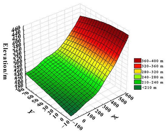
Figure 1.
Topographic map of the permanent plot in a secondary forest in South China. The topographic map was generated from the survey data of the plot using the software Statistica (Version 8.0) (Statsoft, Inc., Tulsa, OK, USA). The X axis represents the northwest-to-southeast direction; the Y axis represents the northeast-to-southwest direction.
2.2. Field Surveys
A total of 400 10 m × 10 m square subplots were established. In each subplot, all individual snags whose DBH ≥ 2.5 cm and whose height ≥ 1 m were sampled. The species of each snag was identified, and their heights (measured to the nearest 0.1 m) and DBH (measured to the nearest 0.1 cm) were measured and recorded.
2.3. Topographic Factors
We recorded topographic factors in each subplot. The elevation, slope aspect, and slope steepness were measured using a total station (Nikon DTM-310, Tokyo, Japan). Slope steepness was classified in accordance with a general classification system—from gentle to very steep. The slope steepness of the four-hectare sample plot ranged from 15.2° to 47.6°, and therefore was classified into three groups: 15–25°, 25–35°, and 35–50°. The elevation ranged from 204 m to 372 m and was classified into four groups: 200–250 m, 250–300 m, 300–350 m, and 350–400 m. Aspect-related thermal gradients shape forest habitats that exhibit heterogeneous energy distributions, thus driving plant structural diversity patterns. The slope aspect of the four-hectare sample plot ranged from 9.8° to 356.6°; from the starting point due north and moving in a clockwise direction, the classifications included the north aspect (338–22°), northeast aspect (23–67°), east aspect (68–112°), southeast aspect (113–157°), south aspect (158–202°), southwest aspect (203–247°), west aspect (248–292°), and northwest aspect (293–337°). The above eight aspects were further divided into four groups: sunny slopes include south aspects, southwest aspects and southeast aspects; semi-sunny slopes include east aspects and west aspects; semi-shady slopes include northwest aspects and northeast aspects; and shady slopes include north aspects [30].
2.4. Analytical Methods
Species abundance, basal area, and density of snags were measured in each subplot. Frequency refers to the percentage of a species among the snags in a sample. Snag diameters were classified into five groups: 2.5–10 cm, 10–20 cm, 20–30 cm, 30–40 cm, and ≥40 cm [31]. Similarly, snag heights were classified into five groups: 1–5 m, 5–10 m, 10–15 m, 15–20 m, and ≥20 m.
The index of dispersion I was used to characterize the spatial patterns of snags. When I ≈ 0, the snags are distributed regularly. Values of I = 1 indicate a random spatial pattern, and values of I greater than 1 present an aggregated spatial pattern [32].
We used a multivariate approach to investigate the relationships between snag distribution and topographic factors. A preliminary detrended correspondence analysis (DCA) was performed to assess the gradient length of the species data for each of the three structural layers. The DCA revealed the presence of large (unimodal) gradients (>4 standard deviations). Hence, to assess the relationships between snag abundance and several topographic factors, we used canonical correspondence analysis (CCA), which is a direct gradient analysis technique that is constrained by a set of a priori environmental characteristics that are hypothesized to influence species distribution patterns. A Monte Carlo permutation test based on 9999 random permutations was performed to test the significance of the eigenvalue of the first canonical axis. Inter-set correlations from the ordination analysis were used to assess the importance of the topographic factors. The CCA was carried out using CANOCO software (version 4.5). A nonparametric Kruskal–Wallis test was used to test the differences in snag distributions between each group of topographic factors. The Kruskal–Wallis test was performed using Statistica software (version 8.0, StatSoft, Inc.). All tests were performed at a significance level of p < 0.05.
3. Results
3.1. Snag Species Composition and Quantitative Characteristics
Data on 544 snags were collected and recorded from 236 subplots in the permanent plot. Forty-four snag species were identified. The overall snags density was 230.5 ± 10.4 snags/ha. Castanopsis carlesii was the most abundant species (90 snags (16.5%) in 53 subplots), followed by Schima superba (30 snags (5.5%) in 21 subplots) and Camellia oleifera (27 snags (4.9%) in 17 subplots). The frequency of each species was calculated as the proportion of subplots in which the species was found, with frequencies of 13.3% (53/400 × 100), 5.3% (21/400 × 100), and 4.3% (17/400 × 100) for Castanopsis carlesii, Schima superba, and Camellia oleifera, respectively. Schefflera octophylla presented the largest basal area (2.66 ± 1.13 m2/ha), followed by Schima superba (1.73 ± 0.40 m2/ha) and Castanopsis carlesii (1.50 ± 0.19 m2/ha). The frequency of Castanopsis carlesii and Schima superba was much greater than that of the other species. The number of snags, accounting for 3.0% of all standing trees, as well as the quantity characteristic of standing trees in the secondary forest plot, is shown in Table 1.

Table 1.
Quantity characteristic of dominant snags of a secondary forest plot in South China.
The snag abundance and richness decreased rapidly as both the snag DBH and height increased. This suggests that tree mortality decreases as tree size increases. The abundance decreased from 408 in the first DBH class to 2 in the ≥40 cm DBH class, indicating a typical reverse-J size distribution (Figure 2A). The most striking feature in Figure 2 is that the abundance and richness strongly decreased from the 2.5–10 cm diameter class. The abundance and richness both strongly significantly differed among the five diameter classes (p < 0.01). The DBH of the snags ranged from 2.5 to 43.5 cm, and the snags of the smallest diameter class (2.5–10 cm) greatly outnumbered those of the other larger-diameter classes. It reflects the reality that trees occupy more space as they grow; hence, plots of a given size will support fewer trees if trees are large compared to when they are small.
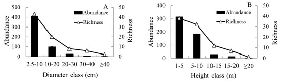
Figure 2.
Distribution of snag abundance and richness across diameter (A) and height classes (B). The diameter and height are both divided into five classes.
The smallest-diameter class (2.5–10 cm) constituted 75.0% of the snags and constituted the most abundant group in our study. We recorded only 10 snags whose DBH was greater than 30 cm; of those snags, only two (0.4%) had a DBH greater than 40 cm, and snags with a DBH ≥ 20 cm constituted only 6.6%. Only two large snags were in the last DBH class, indicating that large snags rarely form. These results indicate that there is a higher mortality among smaller trees and saplings within the community. The abundance decreased from 314 in the first height class to 3 in the ≥20 m height class (Figure 2B), indicating a typical reverse-J size distribution. Both the abundance and richness significantly differed among the five height classes (Kruskal–Wallis test, p < 0.01 and p < 0.05, respectively). The snag abundance decreased as the height increased (Figure 2B). Snags ≤ 10 m in height predominated and constituted 91.7% of the total snag population. We recorded 26 snags that were taller than 15 m and only 3 snags (0.6%) that were taller than 20 m. The results of our study indicated that the snags mostly consisted of individuals with a DBH ≤ 20 cm and a height ≤ 10 m.
3.2. Snag Spatial Distribution Associated with Topographic Factors
The index of dispersion (I = 1.1 > 1) showed that snags were distributed in an aggregated spatial pattern in the sample plots. Of the 400 subplots, 164 contained no snags (41.0%), and approximately 1/5th of the subplots contained one snag (22.0%). Two and three snags were recorded in 16% and 11% of the subplots, respectively.
The results of a CCA (Figure 3) demonstrated that snag patterns were associated with the three measured topographic factors (p < 0.01). The Monte Carlo test (9999 permutations) revealed four significant canonical axes (p < 0.01), which in aggregate explained 6.5% of the variance in species data and 100.0% of the variance in the species–environment relationship (Table 2).
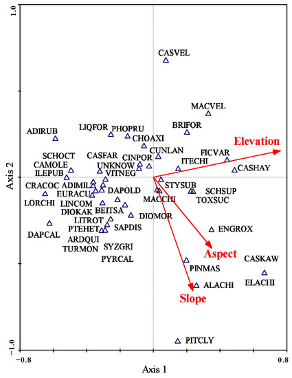
Figure 3.
Two-dimensional ordination diagram of the canonical correspondence analysis (CCA) of 45 snag species recorded in 236 plots as constrained by three topographic factors in a secondary forest in South China. Topographic factors are represented by arrows. The length of an arrow indicates the strength of the correlation between the variable and the axis. Snags species are represented by species codes: Castanopsis carlesii (CASCAR), Schima superba (SCHSUP), Camellia oleifera (CAMOLE), Machilus chinensis (MACCHI), Cunninghamia lanceolata (CUNLAN), Cratoxylum cochinchinense (CRACOC), Cinnamomum porrectum (CINPOR), Pterospermum heterophyllum (PTEHET), Itea chinensis (ITECHI), Schefflera octophylla (SCHOCT), Adinandra millettii (ADIMIL), unknown (UNKNOW), Styrax suberifolius (STYSUB), Engelhardia roxburghiana (ENGROX), Beilschmiedia tsangii (BEITSA), Diospyros morrisiana (DIOMOR), Photinia prunifolia (PHOPRU), Sapium discolour (SAPDIS), Liquidambar formosana (LIQFOR), Litsea rotundifolia (LITROT), Castanopsis fargesii (CASFAR), Lindera communis (LINCOM), Loropetalum chinense (LORCHI), Ardisia quinquegona (ARDQUI), Machilus velutina (MACVEL), Pinus massoniana (PINMAS), Pyrus calleryana (PYRCAL), Adina rubella (ADIRUB), Bridelia fordii (BRIFOR), Choerospondias axillaris (CHOAXI), Diospyros kaki (DIOKAK), Elaeocarpus chinensis (ELACHI), Syzygium grijsii (SYZGRI), Toxicodendron succedaneum (TOXSUC), Alangium chinense (ALACHI), Casearia velutina (CASVEL), Castanopsis kawakamii (CASKAW), Daphniphyllum calycinum (DAPCAL), Daphniphyllum oldhamii (DAPOLD), Eurya acuminata (EURACU), Ficus variolosa (FICVAR), Ilex pubescens (ILEPUB), Pithecellobium clypearia (PITCLY), Vitex negundo (VITNEG), Turpinia montana (TURMON).
Table 2.
Eigenvalues and correlation coefficients for snag abundance and topographic factors (elevation, slope steepness, and slope aspect). * Level of statistical significance: * p < 0.05, ** p < 0.01.
With an eigenvalue of 0.397, the first canonical axis of the CCA explained the most variance in the data. Axis 1 represents the species–environment; strongly positive correlations (r = 0.718) occurred, and the axis explained 66.5% of the species–environment relation. The first axis was strongly significantly correlated with elevation (r = 0.98, p < 0.01) and slope aspect (r = 0.45, p < 0.05). The second canonical axis had an eigenvalue of 0.110 and was significantly correlated with slope steepness (r = −0.70, p < 0.01) and slope aspect (r = −0.43, p < 0.05). The examination of the inter-set correlation (correlations between species axes and environmental variables) and intra-set correlation (correlations between environmental axes and environmental variables) values revealed that both species axis 1 and environmental axis 1 presented the strongest correlations with elevation (r = 0.73 and 0.98, respectively, p < 0.01). Slope steepness and slope aspect were strongly correlated with environmental axis 2 (r = −0.70, p < 0.01 and −0.43, p < 0.05, respectively) and environmental axis 3 (r = 0.65 and −0.78, respectively, p < 0.01). The species distributions in multidimensional space are consistent with the biological characteristics and habitat affinities of individual species. For example, heliophyte species such as Castanopsis carlesii and Castanopsis kawakamii are on the right side of the CCA biplot (sunny aspects and high elevation).
3.3. Relationships between Snags and Topographic Factors
Both the DBH (Kruskal–Wallis test, p < 0.001) and height (Kruskal–Wallis test, p < 0.001) of snags largely varied across the elevation gradient (Figure 4). The mean diameter of snags increased from 4.6 ± 0.3 cm to 11.2 ± 0.9 cm as the elevation increased.
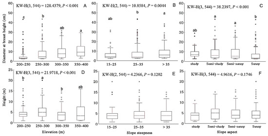
Figure 4.
Response of snags to an elevation gradient according to (A) diameter at breast height (DBH) and (D) height; to slope steepness according to (B) DBH and (E) height; and to slope aspect according to (C) DBH and (F) height. The box plots show the Kruskal–Wallis test results. The horizontal line and small box within each box indicates the median, the box endpoints indicate the 25th and 75th percentile values, and the whiskers represent the non-outlier range; the circles and asterisks indicate the outliers and extreme values of the DBH and height of the snags. Different letters (a, b, c) in the figures represent significant differences between groups (p < 0.05).
The maximum diameter of snags reached 43.5 cm at an elevation of 250–300 m. The average height of snags at an elevation of 250–300 m was significantly higher than that at other elevations. The maximum height of snags reached 20 m.
The DBH largely varied across slope aspect (Kruskal–Wallis test, p < 0.001); however, no significant differences between height and slope aspect were observed (Kruskal–Wallis test, p > 0.05). The DBH and height of snags decreased from shady to sunny aspects, which indicated that, in more mesic plots, snags are much larger and taller.
Similarly, the DBH largely varied across slope steepness (Kruskal–Wallis test, p < 0.05); however, no significant differences between height and slope steepness were observed (Kruskal–Wallis test, p > 0.05). The DBH and height of snags at a 35–45° slope steepness were greater than those at other slope steepness degrees.
4. Discussion
Based on the assumption that trees gain and use the same amount of energy, studies have suggested that tree mortality decreases as tree size increases, and compared with small trees, large trees have an advantage in terms of resource competition [33]. Our research shows that tree mortality tends to decline as tree size increases. However, other studies have reported that, for very large trees, tree mortality is not negatively associated with tree size [34,35]. Among the recorded snags, only 10 (1.8%) had a DBH greater than 30 cm, which supports the conclusion that the size of snags is considerably low in old-growth forests [6]. This phenomenon may be due to differences in climate, site productivity, tree species composition, and disturbance regimes compared to other regions. For instance, the Kanghe Mountains have experienced selective logging, while other regions, such as the Ailao Mountains, have experienced little anthropogenic disturbance. Additionally, topography differs between these regions, with the Kanghe Mountains featuring more undulating terrain and various slope aspects.
The study revealed that topographical heterogeneity, which leads to habitat heterogeneity, was the predominant mechanism generating the spatial distribution of most analyzed species [36]. Snags have shown a consistent aggregated distribution at 0–30-m scales in subtropical mountain forests [20]. Our results also revealed that the spatial pattern of snags was aggregated in the secondary forest of the Kanghe Mountains. Different dead trees showed different spatial patterns: small dead trees presented an aggregated distribution, and large dead trees presented a random distribution [37,38]. The clustered pattern of small snags (DBH ≤ 15 cm) may be explained by the clustered pattern of tree regeneration, and competitive exclusion was the main cause of tree mortality in subcanopy trees. However, the random pattern of large snags may be a consequence of continuous individual tree mortality caused by aging.
The future global extinction risk from climate change is predicted not only to increase but to accelerate as global temperatures increase. Topography-associated thermal gradients predict warming effects on woody plant structural diversity [2]. Other studies have reported a high density of snags at high elevations [39], which contrasts with our results, indicating that snag density decreases as elevation increases.
Our results showed that elevation is an important factor that limits snag distribution in the secondary forest ecosystems of the Kanghe Mountains, which agrees well with many other studies [18,40,41,42,43]. The average DBH and basal area decreased as elevation decreased, which may be due to competition for limited resources. The average height of snags at low elevations was small, possibly because a greater number of species can adapt to low elevations. Competition for limited resources at low elevations limits the growth of individual trees, so the DBH and height of snags remain small.
Our results showed that the abundance of snags was lower on shady slopes than on sunny slopes in the secondary forest of the Kanghe Mountains in South China. However, along the gradient of shady slopes (cold slopes) to warmer slopes, mature trees had significantly fewer stems. Deadwood volume depends on terrain and slope gradient [21]. Aspect-related thermal gradients shape forest habitats that exhibit heterogeneous energy distributions. The energetic equivalence rule supports the hypothesis that elevated temperatures increase the standing stock of species, as these temperatures accelerate the biochemical reactions that govern speciation rates [44].
Light conditions were relatively more abundant on the sunny slopes than on the shady slopes, leading to more intense competition and higher individual mortality in the former; woody plant diversity patterns on small scales is potentially associated with the topographic heterogeneity of energy distribution [45]. Slope aspect and slope steepness represent the horizontal and vertical dimensions of topographic factors, respectively. Temperature clearly changes along the vertical gradient, and vegetation type subsequently exhibits a distinct vertical zonality. Given the multiple functions that snags play in terrestrial systems, knowledge of the factors that affect the distribution of snags is highly important [19,41,46]. An understanding of snag spatial distribution and dynamics, which requires the identification of the factors that influence snag quantity and quality, is difficult to achieve given the numerous factors that simultaneously influence snag distribution.
5. Conclusions
The results of the present study suggest that snags display an aggregated spatial pattern distribution in the subtropical secondary forest in South China, which strongly correlates with elevation, slope steepness, and slope aspect. The snags responded differently to different topographic factors. The number of snags decreased as the elevation increased and tended to increase from shady to sunny slope aspects after logging. However, the DBH of snags showed an opposite trend. Moreover, the snags were tallest at medium elevations and along the steepest slopes. Elevation is an important factor that influences the distribution and growth of snags.
Author Contributions
Conceptualization, L.Z.; Data curation, Y.M., Z.C., S.W., H.L., L.K. and W.D.; Formal analysis, Y.M. and Z.C.; Funding acquisition, L.Z.; Investigation, Y.M., Z.C., S.W., H.L., L.K. and W.D.; Methodology, Y.M. and L.Z.; Project administration, L.Z.; Software, Y.M., Z.C. and S.W.; Writing—original draft, Y.M.; Writing—review and editing, Z.S. and L.Z. All authors have read and agreed to the published version of the manuscript.
Funding
This study was supported by the Forestry Department of Guangdong Province, China, for noncommercial ecological forest research (Grant No: 2020STGYL001) and the Wildlife Conservation and Management Projects of Guangdong Forestry Administration (2022).
Data Availability Statement
Not applicable.
Conflicts of Interest
The authors declare no conflict of interest.
References
- Urban, M.C. Accelerating extinction risk from climate change. Science 2015, 348, 571–573. [Google Scholar] [CrossRef] [PubMed]
- He, S.; Zhong, Y.; Sun, Y.; Su, Z.; Jia, X.; Hu, Y.; Zhou, Q. Topography-associated thermal gradient predicts warming effects on woody plant structural diversity in a subtropical forest. Sci. Rep. 2017, 7, 40387. [Google Scholar] [CrossRef] [PubMed]
- Taccoen, A.; Piedallu, C.; Seynave, I.; Gégout-Petit, A.; Gégout, J. Climate change-induced background tree mortality is exacerbated towards the warm limits of the species ranges. Ann. For. Sci. 2022, 79, 23. [Google Scholar] [CrossRef]
- Stovall, A.; Shugart, H.; Yang, X. Tree height explains mortality risk during an intense drought. Nat. Commun. 2019, 10, 4385. [Google Scholar] [CrossRef]
- Klockow, P.A.; Putman, E.B.; Vogel, J.G.; Moore, G.W.; Edgar, C.B.; Popescu, S.C. Allometry and structural volume change of standing dead southern pine trees using non-destructive terrestrial LiDAR. Remote Sens. Environ. 2020, 241, 111729. [Google Scholar] [CrossRef]
- Bölöni, J.; Ódor, P.; Ádám, R.; Keeton, W.S.; Aszalós, R. Quantity and dynamics of dead wood in managed and unmanaged dry-mesic oak forests in the Hungarian Carpathians. For. Ecol. Manag. 2017, 399, 120–131. [Google Scholar] [CrossRef]
- Ganey, J.L.; Vojta, S.C. Tree mortality in drought-stressed mixed-conifer and ponderosa pine forests, Arizona, USA. For. Ecol. Manag. 2011, 261, 162–168. [Google Scholar] [CrossRef]
- Garber, S.M.; Brown, J.P.; Wilson, D.S.; Maguire, D.A.; Heath, L.S. Snag longevity under alternative silvicultural regimes in mixed-species forests of central Maine. Can. J. For. Res. 2005, 35, 787–796. [Google Scholar] [CrossRef]
- Oberle, B.; Ogle, K.; Zanne, A.E.; Woodall, C.W. When a tree falls: Controls on wood decay predict standing dead tree fall and new risks in changing forests. PLoS ONE 2018, 13, e196712. [Google Scholar] [CrossRef]
- Ohtsuka, T.; Shizu, Y.; Hirota, M.; Yashiro, Y.; Jia, S.G.; Iimura, Y.; Koizumi, H. Role of coarse woody debris in the carbon cycle of Takayama forest. Ecol. Res. 2014, 29, 91–101. [Google Scholar] [CrossRef]
- Romashkin, I.; Shorohova, E.; Kapitsa, E.; Galibina, N.; Nikerova, K. Carbon and nitrogen dynamics along the log bark decomposition continuum in a mesic old-growth boreal forest. Eur. J. For. Res. 2018, 137, 643–657. [Google Scholar] [CrossRef]
- Harmon, M.E.; Fasth, B.; Woodall, C.W.; Sexton, J. Carbon concentration of standing and downed woody detritus: Effects of tree taxa, decay class, position, and tissue type. For. Ecol. Manag. 2013, 291, 259–267. [Google Scholar] [CrossRef]
- Ibarra, J.T.; Novoa, F.J.; Jaillard, H.; Altamirano, T.A. Large trees and decay: Suppliers of a keystone resource for cavity-using wildlife in old-growth and secondary Andean temperate forests. Austral. Ecol. 2020, 45, 1135–1144. [Google Scholar] [CrossRef]
- Kilgo, J.C.; Vukovich, M.A. Can snag creation benefit a primary cavity nester: Response to an experimental pulse in snag abundance. Biol. Conserv. 2014, 171, 21–28. [Google Scholar] [CrossRef]
- Lešo, P.; Kropil, R.; Kajtoch, Ł. Effects of forest management on bird assemblages in oak-dominated stands of the Western Carpathians—Refuges for rare species. For. Ecol. Manag. 2019, 453, 117620. [Google Scholar] [CrossRef]
- Parisi, F.; Frate, L.; Lombardi, F.; Tognetti, R.; Campanaro, A.; Biscaccianti, A.B.; Marchetti, M. Diversity patterns of Coleoptera and saproxylic communities in unmanaged forests of Mediterranean mountains. Ecol. Indic. 2020, 110, 105873. [Google Scholar] [CrossRef]
- Nascimbene, J.; Dainese, M.; Sitzia, T. Contrasting responses of epiphytic and dead wood-dwelling lichen diversity to forest management abandonment in silver fir mature woodlands. For. Ecol. Manag. 2013, 289, 325–332. [Google Scholar] [CrossRef]
- Chmura, D.; Żarnowiec, J.; Staniaszek-Kik, M. Altitude is a better predictor of the habitat requirements of epixylic bryophytes and lichens than the presence of coarse woody debris in mountain forests: A study in Poland. Ann. For. Sci. 2022, 79, 7. [Google Scholar] [CrossRef]
- Sylvain, J.; Drolet, G.; Brown, N. Mapping dead forest cover using a deep convolutional neural network and digital aerial photography. ISPRS J. Photogramm. 2019, 156, 14–26. [Google Scholar] [CrossRef]
- Wu, H.; Franklin, S.B.; Liu, J.; Lu, Z. Relative importance of density dependence and topography on tree mortality in a subtropical mountain forest. For. Ecol. Manag. 2017, 384, 169–179. [Google Scholar] [CrossRef]
- Bujoczek, L.; Bujoczek, M.; Zięba, S. How much, why and where? Deadwood in forest ecosystems: The case of Poland. Ecol. Indic. 2021, 121, 107027. [Google Scholar] [CrossRef]
- Berry, Z.C.; Gotsch, S.G.; Holwerda, F.; Muñoz-Villers, L.E.; Asbjornsen, H. Slope position influences vegetation-atmosphere interactions in a tropical montane cloud forest. Agric. For. Meteorol. 2016, 221, 207–218. [Google Scholar] [CrossRef]
- Suleymanov, A.; Abakumov, E.; Suleymanov, R.; Gabbasova, I.; Komissarov, M. The Soil Nutrient Digital Mapping for Precision Agriculture Cases in the Trans-Ural Steppe Zone of Russia Using Topographic Attributes. ISPRS Int. J. Geo-Inf. 2021, 10, 243. [Google Scholar] [CrossRef]
- Liu, X.; Zhang, W.; Yang, F.; Zhou, X.; Liu, Z.; Qu, F.; Lian, S.; Wang, C.; Tang, X. Changes in vegetation-environment relationships over long-term natural restoration process in Middle Taihang Mountain of North China. Ecol. Eng. 2012, 49, 193–200. [Google Scholar] [CrossRef]
- Lippok, D.; Beck, S.G.; Renison, D.; Hensen, I.; Apaza, A.E.; Schleuning, M. Topography and edge effects are more important than elevation as drivers of vegetation patterns in a neotropical montane forest. J. Veg. Sci. 2014, 25, 724–733. [Google Scholar] [CrossRef]
- Muller, R.N. Landscape patterns of change in coarse woody debris accumulation in an old-growth deciduous forest on the Cumberland Plateau, southeastern Kentucky. Can. J. For. Res. 2003, 33, 763–769. [Google Scholar] [CrossRef]
- Rubino, D.L.; McCarthy, B.C. Evaluation of coarse woody debris and forest vegetation across topographic gradients in a southern Ohio forest. For. Ecol. Manag. 2003, 183, 221–238. [Google Scholar] [CrossRef]
- Kennedy, R.S.H.; Spies, T.A.; Gregory, M.J. Relationships of dead wood patterns with biophysical characteristics and ownership according to scale in Coastal Oregon, USA. Landsc. Ecol. 2008, 23, 55–68. [Google Scholar] [CrossRef]
- Kapusta, P.; Kurek, P.; Piechnik, Ł.; Szarek-Łukaszewska, G.; Zielonka, T.; Żywiec, M.; Holeksa, J. Natural and human-related determinants of dead wood quantity and quality in a managed European lowland temperate forest. For. Ecol. Manag. 2020, 459, 117845. [Google Scholar] [CrossRef]
- Zhang, L.; Ma, D.; Jing, X.L.; Su, Z.Y. Topographic controls on the distribution of indigenous rhododendrons in the southern slope of the Nanling mountains, South China. Pak. J. Bot. 2016, 48, 2367–2374. [Google Scholar]
- Sweeney, O.F.M.; Martin, R.D.; Irwin, S.; Kelly, T.C.; O’Halloran, J.; Wilson, M.W.; McEvoy, P.M. A lack of large-diameter logs and snags characterises dead wood patterns in Irish forests. For. Ecol. Manag. 2010, 259, 2056–2064. [Google Scholar] [CrossRef]
- Taylor, L.R. Aggregation, Variance and the Mean. Nature 1961, 189, 732–735. [Google Scholar] [CrossRef]
- Limin, A.; Slik, F.; Sukri, R.S.; Chen, S.B.; Ahmad, J.A. Large tree species composition, not growth rates, is affected by topography in a Bornean tropical forest. Biotropica 2021, 53, 1290–1300. [Google Scholar] [CrossRef]
- Coomes, D.A.; Allen, R.B. Mortality and tree-size distributions in natural mixed-age forests. J. Ecol. 2007, 95, 27–40. [Google Scholar] [CrossRef]
- Bennett, A.C.; McDowell, N.G.; Allen, C.D.; Anderson-Teixeira, K.J. Larger trees suffer most during drought in forests worldwide. Nat. Plants 2015, 1, 15139. [Google Scholar] [CrossRef]
- Silveira, A.P.; Martins, F.R.; Menezes, B.S.; Araújo, F.S. Is the spatial pattern of a tree population in a seasonally dry tropical climate explained by density-dependent mortality? Austral. Ecol. 2018, 43, 191–202. [Google Scholar] [CrossRef]
- Chen, K.; Zhang, H.; Zhang, B.; He, Y. Spatial distribution and associations of dead woods in natural spruce-fir secondary forests. J. Appl. Ecol. 2021, 32, 2745–2754. [Google Scholar] [CrossRef]
- Von Oheimb, G.; Westphal, C.; Härdtle, W. Diversity and spatio-temporal dynamics of dead wood in a temperate near-natural beech forest (Fagus sylvatica). Eur. J. For. Res. 2007, 126, 359–370. [Google Scholar] [CrossRef]
- Castagneri, D.; Garbarino, M.; Berretti, R.; Motta, R. Site and stand effects on coarse woody debris in montane mixed forests of Eastern Italian Alps. For. Ecol. Manag. 2010, 260, 1592–1598. [Google Scholar] [CrossRef]
- Sefidi, K.; Esfandiary Darabad, F.; Azaryan, M. Effect of topography on tree species composition and volume of coarse woody debris in an Oriental beech (Fagus orientalis Lipsky) old growth forests, northern Iran. iForest—Biogeosci. For. 2016, 9, 658–665. [Google Scholar] [CrossRef]
- Liu, X.; Frey, J.; Denter, M.; Zielewska-Büttner, K.; Still, N.; Koch, B. Mapping standing dead trees in temperate montane forests using a pixel- and object-based image fusion method and stereo WorldView-3 imagery. Ecol. Indic. 2021, 133, 108438. [Google Scholar] [CrossRef]
- Stadelmann, G.; Bugmann, H.; Wermelinger, B.; Bigler, C. Spatial interactions between storm damage and subsequent infestations by the European spruce bark beetle. For. Ecol. Manag. 2014, 318, 167–174. [Google Scholar] [CrossRef]
- Stritih, A.; Senf, C.; Seidl, R.; Grêt-Regamey, A.; Bebi, P. The impact of land-use legacies and recent management on natural disturbance susceptibility in mountain forests. For. Ecol. Manag. 2021, 484, 118950. [Google Scholar] [CrossRef]
- Allen, A.P.; Brown, J.H.; Gillooly, J.F. Global biodiversity, biochemical kinetics, and the energetic-equivalence rule. Science 2002, 297, 1545–1548. [Google Scholar] [CrossRef] [PubMed]
- Carlucci, M.B.; Bastazini, V.A.G.; Hofmann, G.S.; de Macedo, J.H.; Iob, G.; Duarte, L.D.S.; Hartz, S.M.; Müller, S.C. Taxonomic and functional diversity of woody plant communities on opposing slopes of inselbergs in southern Brazil. Plant Ecol. Divers. 2015, 8, 187–197. [Google Scholar] [CrossRef]
- Harmon, M.E.; Franklin, J.F.; Swanson, F.J.; Sollins, P.; Gregory, S.V.; Lattin, J.D.; Anderson, N.H.; Cline, S.P.; Aumen, N.G.; Sedell, J.R.; et al. Ecology of Coarse Woody Debris in Temperate Ecosystems; Academic Press: Cambridge, MA, USA, 1986; pp. 59–234. [Google Scholar]
Disclaimer/Publisher’s Note: The statements, opinions and data contained in all publications are solely those of the individual author(s) and contributor(s) and not of MDPI and/or the editor(s). MDPI and/or the editor(s) disclaim responsibility for any injury to people or property resulting from any ideas, methods, instructions or products referred to in the content. |
© 2023 by the authors. Licensee MDPI, Basel, Switzerland. This article is an open access article distributed under the terms and conditions of the Creative Commons Attribution (CC BY) license (https://creativecommons.org/licenses/by/4.0/).