Article

Intensity Analysis to Communicate Detailed Detection of Land Use and Land Cover Change in Chang-Zhu-Tan Metropolitan Region, China

1
College of Geography and Tourism, Hengyang Normal University, Hengyang 421002, China
2
Hengyang Base of International Centre on Space Technologies for Natural and Cultural Heritage under the Auspices of UNESCO, Hengyang 421002, China
*
Author to whom correspondence should be addressed.
Forests 2023, 14(5), 939; https://doi.org/10.3390/f14050939
Submission received: 2 March 2023 / Revised: 19 April 2023 / Accepted: 23 April 2023 / Published: 3 May 2023

Abstract

:
Quantifying the change in land use and land cover (LULC) is critical for revealing the impact of human activities on the environment of the Earth’s surface. Although some studies were conducted on the change in LULC in rapidly urbanizing areas, conventional methods could not provide a systematic understanding of the changes and their underlying causes. This study adopted an enhanced Intensity Analysis and landscape matrices to deeply explore the change information and expansion modes of LULC in the Chang-Zhu-Tan Metropolitan Region (CZTMR). This exploration was based on remote sensing images from the past 40 years and GIS tools. The results show that the overall change in the LULC accelerated during the period 1980–2020, with its intensity expanding by 16 times. The Built gain and the Crop loss were steadily active. The Built gain was derived mainly from Crop and Forest, and its mode was dominated by edge expansion. It was detected that the Built gain steadily targeted Crop but avoided Forest despite Built gaining a large area from Forest. The reason for this is because Forest initially had the largest area. The measurement results contribute to the formulation of urban plans and land policies for sustainable development in the CZTMR. Our study explained the evolution of Intensity Analysis and its analytical thought, which could be employed in other regions for the detection of land change to help decision makers develop more targeted and sustainable land management strategies.

1. Introduction

Rapid urbanization comes with successful socioeconomic development but profoundly intensifies the evolution of global land use and land cover (LULC) [1]. A change in LULC reflects landscape dynamics on the Earth’s surface and significantly impacts global ecosystems, food security, climate change, and biodiversity [2]. At the same time, urban areas and their inhabitants face severe risks due to these effects [3]. Thus, quantifying and understanding the spatiotemporal dynamics of LULC is critical in revealing the interaction mechanism between human activities and the natural environment [4,5]. Measuring LULC change information is not only important for identifying land transformation characteristics but is also an indispensable step in revealing the factors influencing land change, evaluating the impact of change on ecosystem services, and modeling change projections [6,7,8,9]. Hence, it is crucial to quantify land change in a straightforward and detailed way.
The most practical approach to analyzing the change in LULC is to access maps of Time 1 and Time 2 and then examine these changes, using a transition matrix to identify the most important transitions [10]. Finally, scientists investigate the processes that produced these transitions. The transition matrix (also known as cross-tabulation) method is widely employed to analyze differences in the size of transitions among LULC categories at a single time interval [10,11,12]. As traditional analyses typically concern the size of the transition, scientists tend to detail the larger transitions and neglect the smaller ones [13]. For example, when Xie et al. [14] investigated transitions among different LULC categories in Wuhan, they detailed the categories that experienced more significant changes and analyzed their influencing factors. Yu et al. [15] applied the size of the change in the transitions to detect the contributions of the impact of land cover change to the land surface temperature. Some studies identified the main land transitions of LULC via the size of change to forecast categorical land change [16,17,18]. These studies believed that a larger change is a more considerable sign of dramatic land changes. Though the size of the change is intuitive, it cannot convey useful information about the proportion of the size of the change in the category’s area to the category’s area. Therefore, it is hard to effectively characterize the intensity of change in LULC categories. More and more scientists have suggested that the intensity (proportion) of the change might be more meaningful than the size of the change for understanding the processes and causes of LULC change. Unlike conventional methods and models, Aldwaik and Pontius Jr. [19] proposed an Intensity Analysis to ascertain which changes and transitions of categorical land dynamics are more intense. This method is a hierarchical framework for the detection of the size, intensity, temporal stationarity in the time interval, category, and transition level of land change [20,21]. It can compensate for the limitations of traditional measurements [22] and has been extensively applied worldwide [23,24,25,26,27]. This advanced analytical technique has advantages in identifying historical land use classification errors [28] and explaining the results of changes in LULC dynamics [29]. Some scholars have also applied the method to investigate urban expansion intensity [30], the dynamic characteristics of desertification [31], and regional comparisons [22,32,33].
Early versions of the Intensity Analysis, which emerged from earlier measurements of single intervals, have achieved popularity [34,35,36,37]. Nevertheless, interpreting the Intensity Analysis is more straightforward because of its clear hierarchies, graphical expressions, and, in particular, more insightful explanations of the causes of temporal changes in LULC [26,38,39]. For example, why is the transition size from category M to category N larger than the transition size from other categories to category N? There are two reasons for this [33]. Firstly, suppose category M has a larger area than the other categories at the initial point. In that case, it naturally has more area to transition to N. Therefore, even if category N gains transited area from the other categories at a uniform transition intensity, category N will also gain more area from category M. Secondly, at the initial point, category N gains transited area from category M at a greater transition intensity compared to the other categories. Sometimes these two situations may exist simultaneously. Intensity Analysis provides a pathway for scientists to associate patterns with processes [40]. To reflect the stationary characteristics in detail and intuition, Deng and Quan (2022) proposed a novel “transition pattern” to enrich the original Intensity Analysis [20] which can help decision makers formulate more targeted management strategies and improve the reliability of the simulated results via modeling to emphasize the stationary process of the change.
Chang-Zhu-Tan is a rapidly developing region in central China. Massive rural populations migrated to the urban area, and the urban sprawl has encroached on many other lands over the last four decades, leading to a series of concerns such as local climate change, water shortages, and air pollution. These issues have brought challenges with fulfilling the sustainable development goals (SDGSs e.g., 11.3, sustainable urbanization). Most existing studies in the Chang-Zhu-Tan area focused on the change in a single category, such as built-up land, and they carried out research on the scales of the Chang-Zhu-Tan urban agglomeration and the central region of Changsha. Moreover, these research studies were mainly concentrated on the assessment of ecosystem services [41,42], urban land scenario projections [43,44], the delineation of urban growth boundaries [45], and land use carbon emissions [46]. However, few studies have reported on an in-depth analysis of the change in LULC over a long time series at the scale of the metropolitan region. In February 2022, the development plan of the Chang-Zhu-Tan Metropolitan Region was officially approved by the Central Government of China, making the Chang-Zhu-Tan Metropolitan Region (abbreviated as CZTMR) the first Metropolitan Region in central China [47]. The establishment of the CZTMR aims to expedite the pace of integration in the future, which inevitably accelerates urban area growth and causes tremendous pressure on the ecological environment. Therefore, for the rapid expansion and sprawl of urban areas, it is natural to raise questions. (1) How do the size and intensity of changes in LULC vary temporally in the CZTMR? (2) What are the patterns and processes of urban sprawl and its possible causes over the past 40 years?
To solve the problems above, we took the CZTMR as a case study and combined the enhanced Intensity Analysis with landscape matrices to better evaluate the LULC change in the CZTMR. Specifically, the two objectives of this study were to analyze the size, intensity, and stationary characteristics of the changes in the LULC during the period of 1980–2020 and reveal how processes of urban expansion affect the changes in the landscape pattern in the CZTMR. This topic is of major importance in the CZTMR for providing a scientific basis for eco-environmental protection and sustainable urban development.

2. Materials and Methods
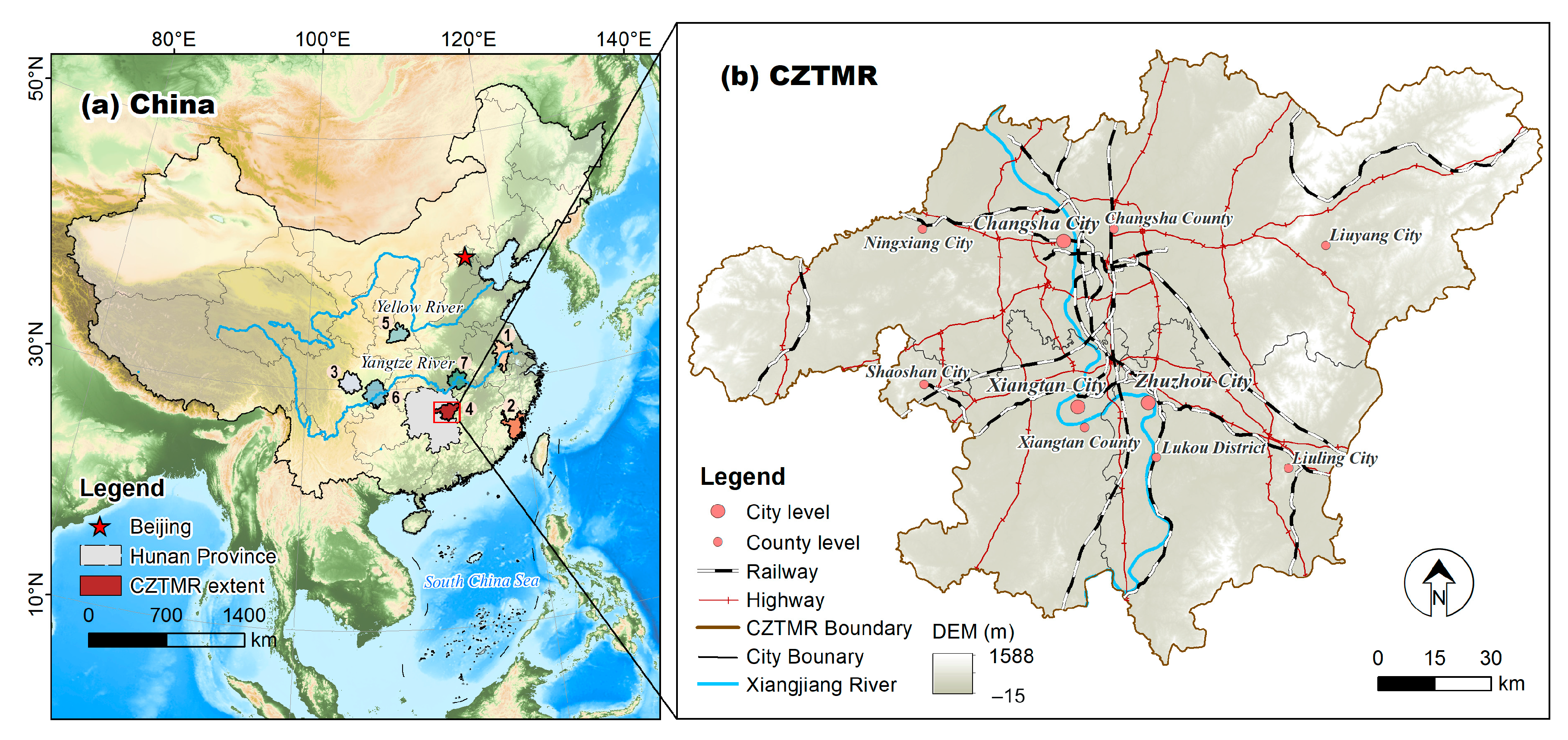
2.1. Study Area

This study took the regional extent of the CZTMR delineated in the development plan of the Chang-Zhu-Tan Metropolitan Region as the study area. The CZTMR includes the whole of Changsha City, the central urban areas of Zhuzhou City, Liling City, Xiangtan City, and Shaoshan City, and Xiangtan County, with a total area of 18,900 km2 (Figure 1). The CZTMR is a fundamental unit of urban agglomerations in the middle reaches of the Yangtze River in the northern-central Hunan Province, located between 111°53′32″~114°15′28″ E and 27°13′31″~28°39′56″ N. It is also one of the core forces for the promotion of the synergistic development of the Yangtze River economic belt. In 2021, the population was 14.84 million, with an urbanization rate reaching 80.9% and a GDP of CNY 1.79 trillion, accounting for 40% of the province’s total economy [48]. For industry scale, the CZTMR’s engineering and machinery industries ranked first in China for a long time. In addition, its transportation advantage is prominent, with the Beijing–Guangzhou and Shanghai–Kunming high-speed railways and the intersections of many other transportation road networks.

2.2. Data Source and Processing

The framework diagram of this study is shown in Figure 2. The LULC data were obtained from China’s Multi-Temporal Land Use/Land Cover Remote Sensing Monitoring Database by the Resource and Environmental Science Data Centre of the Chinese Academy of Sciences (http://www.resdc.cn, accessed on 11 March 2022). These data are based on a Landsat TM/ETM+/OLI multitemporal image interpreted via human–computer interaction with a spatial resolution of 30 m. The mapping accuracy of the LULC category in level II is above 90% [12,49,50]. Five time points of LULC data were used in this study: 1980, 1990, 2000, 2010, and 2020. The regional administrative boundaries, transport infrastructure such as railways and highways, and government location data were downloaded from the National Geographic Information Centre’s National Geographic Information Resources Catalogue Service (http://www.webmap.cn, accessed on 18 March 2022). DEM data at a resolution of 30 m were derived from the ASTER GDEM data product on the United States Geological Survey (USGS) website (https://earthexplorer.usgs.gov, accessed on 26 May 2022). The land classification system categories are Crop, Forest, Grass, Water, and Built and are based on ground surveys and previous research in the study area [42,44].

2.3. Methods

2.3.1. Intensity Analysis

The methodology of Intensity Analysis based on a transition matrix consists of a hierarchical, top-down interval level, category level, and transition level [33,51]. The interval level is designed to analyze which intervals are fast or slow for the total change in LULC. The category level can further analyze which categories are active or dormant for the gains and losses of LULC categories. The transition level provides deeper insight into whether transitions from other categories to a particular category are targeted or avoided. This study adopted this method to characterize the intensity of the change in LULC dynamics. This method program was designed based on the R language package and is available on the website (www.clarku.edu/~rpontius, accessed on 14 July 2022).
The interval level examines the differences in the total change over multiple intervals. The total change intensity St for a single interval and the uniform intensity U for all intervals are calculated in Equations (1) and (2), respectively [19,52]. The total change in a single interval is determined to be fast or slowvia a comparison of the magnitude of St with U. If St > U, the interval’s change in the overall interval is fast; if St < U, the interval’s change in the overall interval is slow.
S t = c h a n g e   s i z e   a t   i n t e r v a l   [ Y t , Y t + 1 ] / Y t + 1 Y t s i z e   o f   s t u d y   r e g i o n × 100 %
U = s u m   o f   c h a n g e   s i z e   a t   a l l   i n t e r v a l s / ( Y T Y 1 ) s i z e   o f   s t u d y   r e g i o n × 100 %
where t ranges from 1 to T − 1 and is an index for the initial time point; T is the number of time points for the LULC maps; Yt is the year in time point t. The interpretation of these symbols can apply to Equations (3)–(6).
The category level can investigate the differences in the category change via gain and loss. Equations (3) and (4) define the annual loss intensity for category i and the annual gain intensity for category j, respectively [19,52]. The loss and gain for a category are judged to be active or dormant through a comparison of the magnitudes of Li and Gj with St. The loss for category i is active if Li > S; otherwise, the loss for category i is dormant. Determining the category’s loss is suitable for the category’s gain.
L t i = G r o s s   l o s s   s i z e   f o r   c a t e g o r y   i   a t   i n t e r v a l   [ Y t , Y t + 1 ] ( Y t + 1 Y t ) s i z e   f o r   c a t e g o r y   i   a t   i n i t i a l   t i m e   o f   i n t e v a l   [ Y t , Y t + 1 ] × 100 %
G t j = G r o s s   g a i n   s i z e   f o r   c a t e g o r y   j   a t   i n t e r v a l   [ Y t , Y t + 1 ] ( Y t + 1 Y t ) s i z e   f o r   c a t e g o r y   j   a t   f i n a l   t i m e   o f   i n t e v a l   [ Y t , Y t + 1 ] × 100 %
In this study, the transition level was used to evaluate the difference in the transitions from the other non-Built categories to the Built category. Equations (5) and (6) define the intensity of the transition from category i to category n and the uniform transition intensity from other categories excluded from category n to category n, respectively [19,52]. The category i transiting to category n is targeted, and category n’s gain targets category i if Rin > Wn; otherwise, the category i transiting to category n is avoided, and category n’s gain avoids category i.
R t i n = s i z e   o f   t r a n s i t i o n   f r o m   c a t e g o r y   i   t o   n   a t   i n t e r v a l   [ Y t , Y t + 1 ] / Y t + 1 Y t s i z e   f o r   c a t e g o r y   i   a t   i n i t i a l   t i m e   o f   i n t e r v a l   [ Y t , Y t + 1 ] × 100 %
W t n = s i z e   o f   t r a n s i t i o n s   f r o m   o t h e r   c a t e g o r i e s   t o   n   a t   i n t e r v a l   [ Y t , Y t + 1 ] / Y t + 1 Y t s i z e   f o r   o t h e r s   e x c l u d e d   f r o m   c a t e g o r y   n   a t   i n i t i a l   t i m e   o f   i n t e r v a l   [ Y t , Y t + 1 ] × 100 %

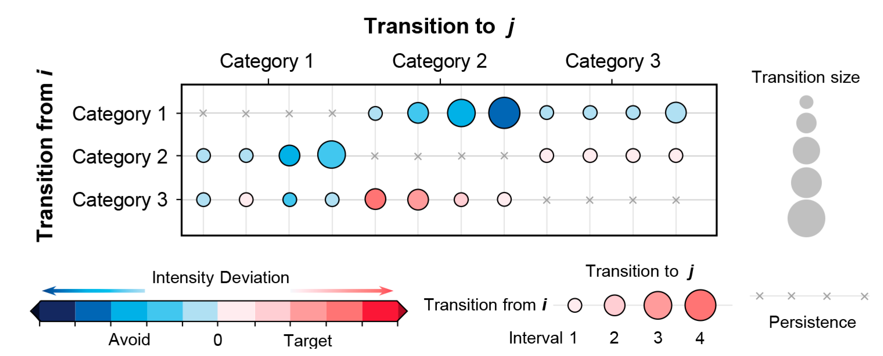
2.3.2. Transition Pattern

Given that the transition level of the original Intensity Analysis cannot be comprehensive and intuitive to represent the size, intensity, and stationarity of various transitions, this study employed a novel transition pattern approach to characterizing the transition for LULC [20]. Figure 3 describes the transition pattern. In Aldwaik and Pontius Jr. (2012) [19], the stationarity of the LULC transition was defined as the transition from category i to category j that is greater or less than the corresponding uniform intensity at all intervals. If all are greater than the uniform intensity, the transition is stationary targeting; otherwise, the transition is stationary avoiding. The rows and columns in Figure 3 represent the category at an initial time and the category at a final time, respectively. The bubble scale represents the size of the transition; the bubble’s color represents the degree to which the transition intensity deviates from the corresponding uniform intensity and can reflect the degree to which the transition is targeted or avoided. By comparing the bubbles’ colors horizontally, investigators can identify the stationarity of the transition process during the overall period.

2.3.3. Spatial Mode of Landscape Expansion

Urban expansion is frequently driven by socioeconomic factors, natural resources, transport infrastructure, geographical location, eco-environment, urban planning, and policy. Its growth mode is diverse. Liu et al. (2012) summarized the urban expansion process into three main modes: infilling, edge expansion, and outflying (Figure 4) [53]. The landscape expansion index (LEI) can help scientists determine the spatial expansion mode of a new patch of Built land. If LEI = 0, the new patch belongs to the outflying mode; if 0 < LEI ≤ 50, the new patch belongs to the edge expansion mode; if 50 < LEI ≤ 100, the new patch belongs to the infilling mode. The study applied the area-weighted mean expansion index (AWMEI) to capture the agglomeration process of the Built expansion in this study. If the value of AWMEI decreases, the development of the Built expansion is diffused; If the value of AWMEI increases, the development of the Built expansion is compact [53].
L E I = 100 × A o A o + A v
A W M E I = i = 1 n L E I i × a i A
where LEI is the expansion index of the newly Built patches, Ao is the intersection between the buffer zone and its overlayed part, and Av is the intersection between the buffer zone and its non-overlayed part. LEIi is the LEI of the newly Built patch i; ai is the area of the newly Built patch i; A is the total number of the newly Built patches. The increasing value of AWMEI indicates that the expansion and sprawl of the Built land have a compact trend; inversely, the decreasing value of AWMEI indicates that the Built area’s expansion and sprawl have a diffuse trend.

2.3.4. Landscape Pattern Matrices

The landscape pattern matrix is a series of indicators that can quantitatively describe spatial patterns for categorical variables [54]. The LULC observation data were converted into Tiff format using ArcGIS Pro software (Version 2.5, Esri, Redlands, CA, USA). We calculated the pattern indexes at the class and landscape levels based on Fragstats software (Version 4.2, Portland, OR, USA). In this study, we selected the indexes, including the number of patches, patch density, mean patch size, edge density, fractional dimension, aggregation index, Shannon’s diversity index, and Shannon’s evenness index. The above eight indexes can acquire the landscape fragmentation, geometry, diversity, and aggregation of the LULC in the CZTMR.

3. Results

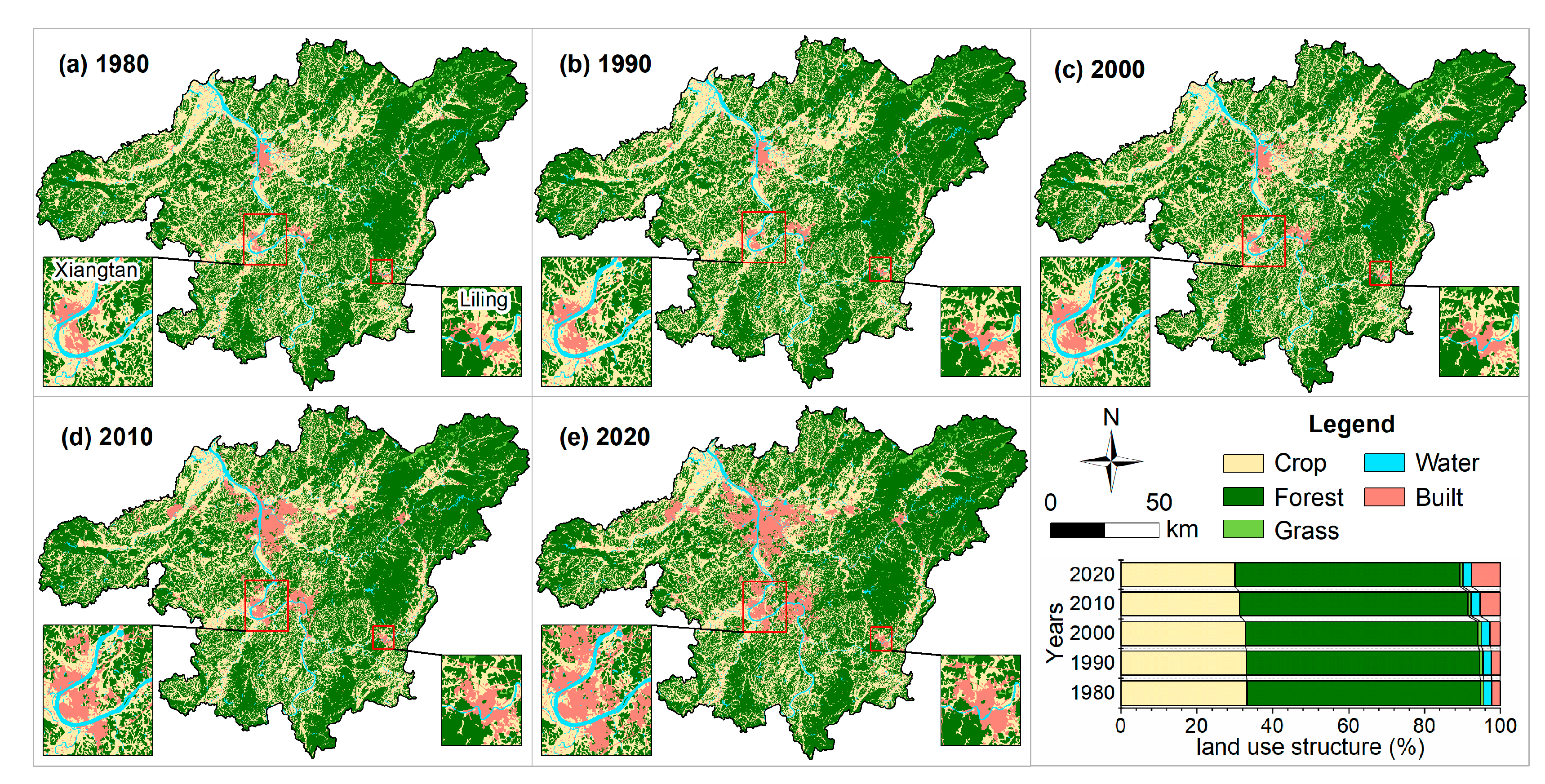
3.1. LULC Structure Analysis

Figure 5 shows the LULC structure and its spatial pattern. During the period 1980–2020, the largest category in LULC area was Forest, followed by Crop. They comprise approximately 90% of the study area, indicating that the ecological resources in this region are widely distributed and have an excellent resource endowment. The growth of Built continues to rise, with the proportion increasing from 2.2% in 1980 to 7.52% in 2020.
In contrast, Crop and Forest shrunk from 33.3% and 61.5% in 1980 to 30.0% and 59.3% in 2020, respectively. A zoomed-in view of Figure 5 reveals the rapid outward expansion and sprawl of the Built category in both Xiangtan and Liling Cities, encroaching by degrees on the adjacent ecological environments, such as Crop and Forest. This reflects that the growth in the quantity of Built land is the most significant feature in the CZTMR, despite having had a small proportion in 1980.

3.2. Detection of LULC Change Size and Intensity

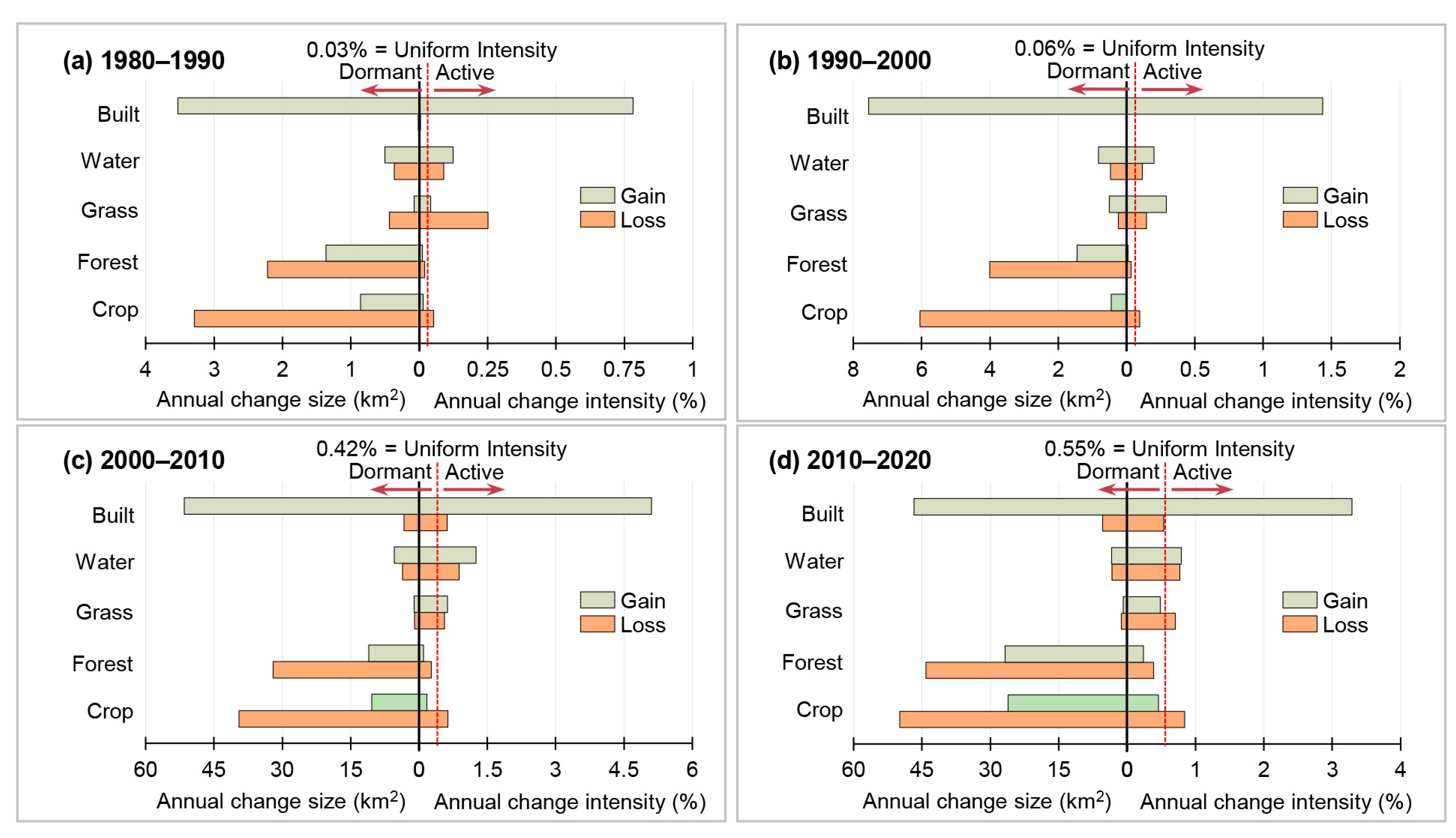
3.2.1. Change Detection at Time Interval Level

Figure 6 shows the size and intensity of the LULC’s total change at four intervals. As shown in Figure 6, the size and intensity of the change in the LULC show an increasing trend. The total change demonstrated non-stationary characteristics during the overall period since the change intensities at four periods are not equal to the uniform intensity (0.26%) on the right side of Figure 6. Interestingly, after 2000, the size and intensity of the change increased sharply, from an annual change size of 6.32 km2 from 1980 to 1990 to 103.90 km2 from 2010 to 2020. This suggests that the total change in the former two intervals was relatively slow compared to the change in the latter two.

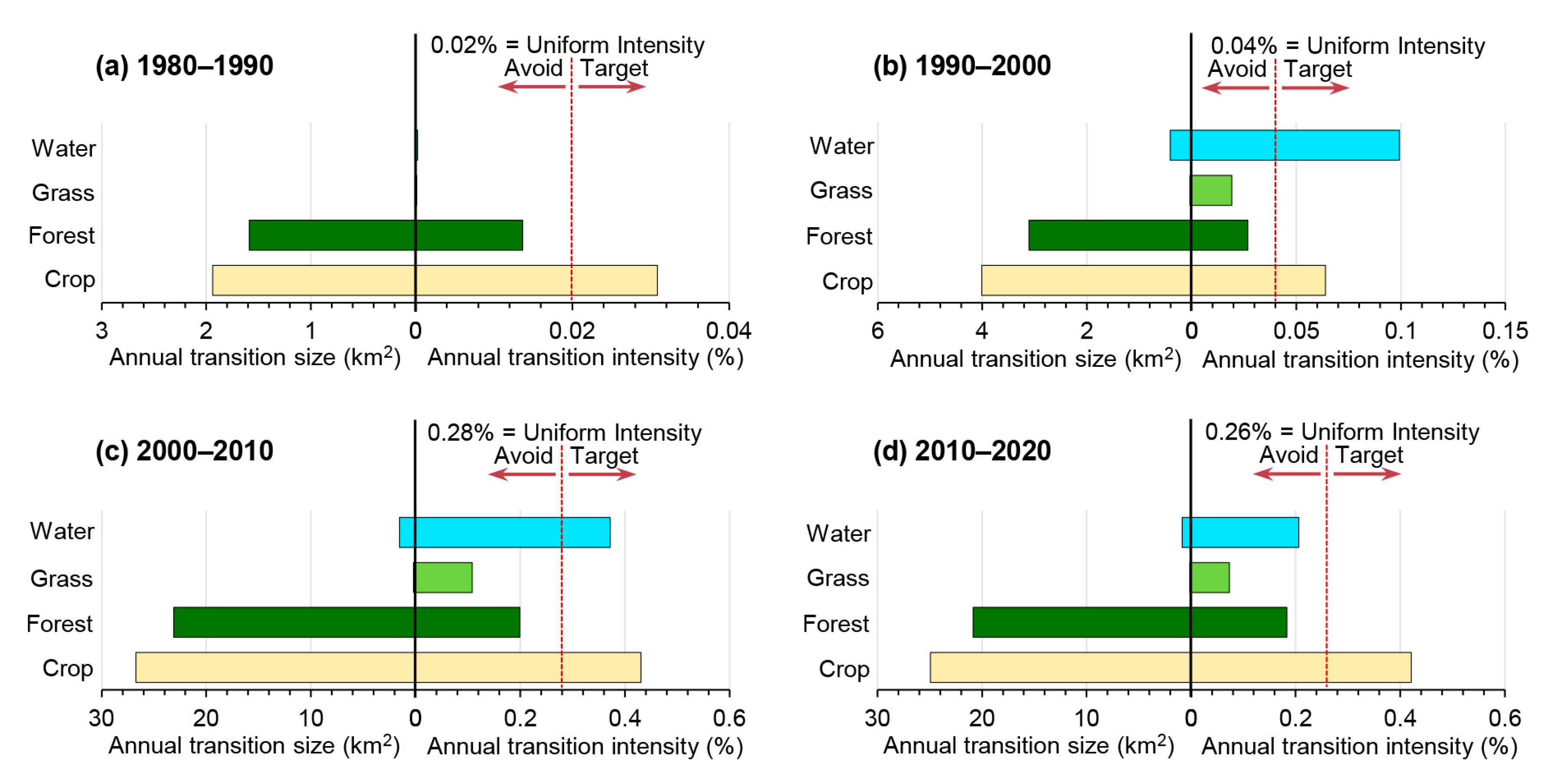
3.2.2. Change Detection at Category Level

The annual sizes of the Built gain at four intervals from 1980 to 2022 were 3.5 km2, 7.6 km2, 51.6 km2, and 46.8 km2, respectively (Figure 7). Its gain intensity far exceeds the uniform intensity, with an increasing trend from 1980 to 2010. Furthermore, the loss size and intensity of the Built area are much smaller than its gain, further reflecting the quantitative growth of the Built category with active status.
Conversely, the intensities of Forest’s gain and loss are less than the uniform intensity at all intervals, although the sizes of the gain and loss for Forest are not insignificant. Hence, the gain and loss of Forest are stationary and dormant. Forest’s loss is greater than its gain over the whole period, resulting in a net loss. The loss intensity of Crop is more robust than its gain intensity. As the loss intensity of Crop is always greater than the uniform intensity, it behaves as stationary and active. There is a tendency to find a steady increase in the gain of Crop, which is possibly related to the decisive implementation of the land policy of balancing between occupation and compensation for Crop and the gradual popularization of sustainable land development since the 21st century. The Water net increased slightly its gain exceeded its loss. Regarding Grass, its gain intensity is greater than the uniform intensity except for the fourth interval.

3.2.3. Change Detection at Transition Level

On the left side of Figure 8, the annual sizes of the transition from Crop to Built at four intervals are 1.94, 4.00, 26.73, and 24.93 km2, respectively, showing a trend of increasing first and then decreasing. The Built gain targeted Crop because its transition intensity was always greater than the uniform intensity. Instead, the Built gain steadily avoided Forest as its transition intensity was less than the uniform intensity at all intervals. Nevertheless, the size of the transition from Forest to Built is enormous, with annual areas of 1.59, 3.11, 23.10, and 20.84 km2 at four intervals, respectively.
Additionally, Built’s gain steadily avoided Grass. The differences at intervals for the transition intensity from Water to Built indicates that Water underwent a slight change to a drastic change and a slight change transition process. The uniform intensity changes of its transition to Built describe the aggressive dynamic of the Built expansion.
Figure 9 shows the transition pattern of the LULC throughout the study period. The novel transition pattern represents the size and intensity of the categorical transition via the scale and color of the bubbles. Checking the color consistency in the horizontal direction can identify the stationary characteristic. It is shown in Figure 9 that not all of the LULC transitions are stationary. Among them, some transition processes show a stationary targeting characteristic: the transition of Crop to Water, the transition of Crop to Built, the transition of Forest to Grass, the transition of Grass to Forest, and the transition of Water to Crop. Other transition processes show a stationary avoiding characteristic: the transition of Crop to Grassland, the transition of Forest to Crop, the transition of Forest to Water, the transition of Forest to Built, the transition of Grass to Built, the transition of Water to Forest, and the transition of Built to Grass.

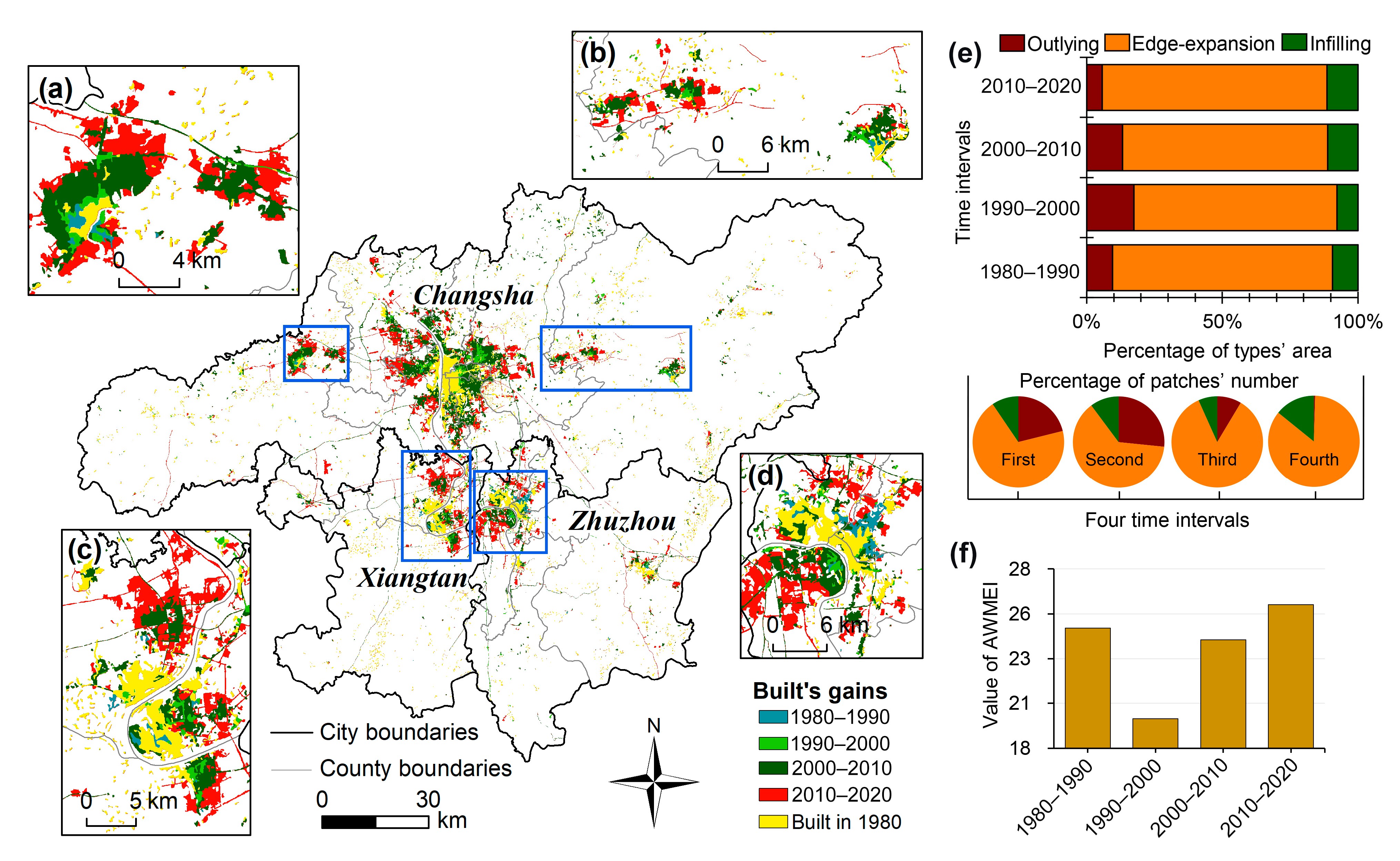
3.3. Dynamic Process of the Built Expansion

Figure 10 shows the Built expansion process and its mode at different intervals. As shown in Figure 10, the Built expansion is a distinct process that continues to sprawl outwards, occupying other categories, especially Crop, followed by Forest.
From 1980 to 2020, there was an apparent eastward expansion of Built land owing to policy influences and the economic growth needs in Ningxiang (Figure 10a). Consequently, a significant economic and technological development zone (dominated by food and beverage processing) was established between Ningxiang and Changsha to promote regional manufacturing. Liuyang displayed a westward expansion to receive radiation from the economic development of this core (Figure 10b). As a result, an enormous economic and technological development zone (dominated by the biomedical industry) also formed between Liuyang and Changsha. Moreover, the expansion of Xiangtan to the north is evident in Figure 10c. Zhuzhou shows an expansion of the Built environment from the north bank to the south bank of the Xiangjiang River (Figure 10d). This expansion is attributed to the more complicated topography and Forest on the north bank compared to the Crop land in the flat area on the south bank, which makes it difficult and costly to develop. Figure 10e shows that the edge-expansion mode area exceeds 75% of the new Built land during four intervals, with the maximum (83%) reached during the 2010–2020 period. This reflects that the edge-expansion type dominates the spatial expansion mode of the Built category.
Regarding the number of new patches of different expansion modes, the edge-expansion type still dominates, while outflying expansion shows a trend of first increasing and then decreasing. The AWMEI of Built expansion tends to decrease and then increase, reaching a maximum during 2010–2020, demonstrating that the growth of Built land in the study area exhibits a more compact development pattern due to the increase in the infill expansion area (Figure 10f).

3.4. LULC Pattern Analysis

Figure 11 shows the spatial pattern trend at the class level from 1980 to 2020. As shown in Figure 11a,b, the Built patch density maintains a relatively high level. Nevertheless, its mean patch size continues to grow, indicating that the landscape fragmentation of Built declines while the degree of aggregation rises. The patch densities of Crop and Forest have increased remarkably since 2000. Meanwhile, the mean patch sizes show a distinct decrease, indicating that the fragmentation of Crop and Forest is intensifying, with the number of more significant ecology patches decreasing. Figure 11c,d show that the edge density values for Crop and Forest are more prominent throughout the period, which may be related to their proportion of the area. In addition, the edge densities and fractional dimensions of Built and Water appear to increase and are clearer for Built. From 1980 to 2020, it is clear that the transport land (the line symbolized in red) of the Built area has increased (Figure 10). Categories with a linear shape often have higher edge densities and fractional dimensions; hence, the shape of the Built area becomes more complex.
The overall characteristic is that the turning point of the LULC landscape change LULC is around 2000 (Figure 12). Specifically, at this point, the density and number of patches gradually increase; conversely, the mean patch size displays a decreasing trend. This suggests an increased fragmentation of the overall landscape in the CZTMR. When the edge density tends to rise, the patch shape complexity is increased (Figure 12c). The aggregation index and the contagion show slight fluctuations, followed by a decline. Together, the Shannon diversity index (SHDI) and the Shannon evenness index (SHEI) can characterize the landscape’s diversity, and they indicate that the landscape diversity increased over the study period, with a balanced development trend for various land categories.

4. Discussion

4.1. Intensity Analysis Compared with Other Methods

With the rapid growth of the urban population and socioeconomic development, human activities are altering LULC at an unprecedented size, intensity, and spatial extent [1]. The intensity of the land change is a vital signal for detecting and appraising categorical land variations. It can characterize the dynamic process of the spatial extent using land categories and the transition between land categories [20]. This study discusses methods related to the detection of change after classification based on remote sensing images rather than detecting change by applying remote sensing images directly. Until now, most of the indicators and methods for detecting land change reflected the intensity of the change to various extents, such as the transition matrix [50], the change area of the category’s extent [55], the single and comprehensive land use dynamic degree (SLUDD, CLUDD) [56], systematic transition analysis [36], and Intensity Analysis adopted in our study. In conventional research on land change, one current thought is that the transition size in the transition matrix is a signal of the intensity of land transition [13]. For example, Zhang et al. investigated land use transitions in Hengyang during the 2010–2015 and 2015–2018 periods [57]. They found that the transition of Woodland to Construction land was the largest, but a deeper analysis can generate more insightful interpretations [20]. We analyzed the transition matrix during the two periods in their study using Intensity Analysis, which identified that the transition from Arable land to Construction land was more intense than the transition from Woodland to Construction land. Since the gain of Construction land steadily avoids Woodland, the enormous loss of Woodland to Construction land can be explained by the greater initial size of Woodland.
In the transition matrix, the total column and row provide the most general information: the quantity of each category at an initial time and a final time, respectively. The net change is the difference between them, and its analysis also is a prevalent study [58,59]. A lack of net change does not necessarily represent a lack of change in a category, although the net change can be helpful. A land category’s total quantity may mostly stay the same at a time interval. However, it may undergo significant exchange changes, losing a certain amount to other land classes while gaining an equal amount from them in different locations. The SLUDD is the annual net change for one category as a proportion of the category’s size at the initial time, and it is widely used to express the intensity of the category’s change [12,60]. The SLUDD can show a positive or negative net change. However, the degree does not synchronously portray the category’s loss and gain, so it lacks the exchange component of change that is vital information. The category’s total change contains its gain and loss instead of the net change [61].
Moreover, the SLUDD is confusing, as the gain part of the category is not directly related to its initial status but constitutes the final status, and the lost part of the category is necessarily composed of its initial status. In essence, the CLUDD is the sum of the loss intensities of different categories [22]. Scientists frequently employ it to compare the intensities of the total change at different intervals [50,62]. Nevertheless, it underestimates the actual change occurring at a time interval because it misses the gain component of the total change. Some scientists discovered that the CLUDD needs more practical interpretation by comparing the CLUDD with Intensity Analysis methods in Longhai, China [22]. Furthermore, Pontius Jr. et al. demonstrated that the CLUDD is confusingly vague and easily misleads readers with unclear mathematical expressions [63].
We have tracked the evolution of the Intensity Analysis and found some concerns that require significant attention in some of the literature regarding the use of this method. The early version of the Intensity Analysis was known as the systematic transition analysis. Scientists adopted the early version extensively to identify systematic versus random transitions between categories. As the method only analyzed transition level information, it is therefore no longer suitable for researchers and decision makers who want to detect the land change in detail. Aldwaik and Pontius Jr unified the size, intensity, and temporal stationarity at the interval, category, and transition levels of land change [19]. They also proposed systematic characteristics based on Intensity Analysis [28]. The systematic characteristics of the land transition were first defined by Alo and Pontius Jr. [34]. The transition from category m to category n is a systematically targeting transition in which the gain of n targets m while n targets the loss of m, i.e., when Rtmn > Wtn and Qtmn > Vtm [28]. Qtmn and Vtm are defined in detail in Equations (7) and (8) of Aldwaik and Pontius Jr. [19]. Precisely, Qtmn equals the annual area of transition from category m to n as the percentages of the sizes of the category n at the end of the time interval. The systematic criterion is the investigation of a category’s transitions with respect to the category’s loss and gain. For example, the transition from Crop to Forest is analyzed from two perspectives: the loss of Crop and the gain of Forest. However, many subsequent works have shown that the perspective for the category’s loss should be removed from the transition level of Intensity Analysis [24,64,65,66]. Quan et al. [33] realized that the transition intensity for a category’s loss did not have a precise interpretation when analyzing temporal change because the transition process influences the category’s end size during the time intervals. However, they still applied the definition to analyze the systemic characteristics of categorical land transition in their studies [27,67,68,69,70]. The definition of “systematic” and the transition intensity of a losing category should be eliminated when using Intensity Analysis to detect land changes. Therefore, this study also aims to remind scientists that they can consider this issue when using the method. Finally, we consider that a good method for detecting land changes should include at least five characteristics:
  • Containing information on the size and the intensity of a change rather than only evaluating the size of change;
  • Distinguishing the losses and gains of land categories instead of focusing only on net change;
  • Providing multiple levels of connectivity, allowing scientists to carry out any levels of land change analysis according to the needs of their study;
  • Comparing and analyzing the overall change in LULC during different periods;
  • Facilitating the comparison of land change patterns and processes across regions to help guide the design of regional land management policies.

4.2. Patterns and Processes of LULC Change

The results of the intensity of LULC change show a significant acceleration in the overall speed of change in the two intervals after 2000 (Figure 6). The change in value in the pattern indexes in Figure 11 and Figure 12 also demonstrates a turning point in change around the year 2000. This change might be closely associated with population growth and economic development. At the category level, the Built category has the largest gain; conversely, Crop demonstrates the largest category loss. Forest is declining over a large area, undergoing a dormant decrease. The process is described as the “large dormant category phenomenon” [29]. At the transition level, the gain of Built derived mainly from Crop and Forest (Figure 9), while the landscape fragmentation of Crop and Forest intensified (Figure 11). The likelihood of Crop being encroached upon or abandoned might then increase because smaller patches are more vulnerable to being occupied by dominant neighbor patches and are easily ignored by land regulators. As seen in Figure 8, the transition from Crop to Built shows stationary targeting. This transition might be closely related to urban–rural population migration. Figure 13a shows that in Chang-Zhu-Tan, the total population has steadily increased since 1984. The increased speed of the urban population during the period of 2001–2019 is three times the speed that during the 1984–2000 period in the region. Figure 13b shows that economic development has become a more rapid process since the 21st century. The sharp increase in the urban population has caused the need for more housing, transportation, and other infrastructures to meet the needs of human activities. The process is also interpreted as population urbanization driving land urbanization forward [71].
Moreover, this study found that the intensity of the transition from other categories to the Built category increased in the early three intervals but decreased in the fourth interval (Figure 9). This is possible response to the national emphasis on the shift from incremental to stock planning for the quality of the Built category in recent years. The transition pattern in Figure 8 also suggests the gain of Built targeted Crop during 2000–2010 and 2010–2020. In the urbanization scenario, Built seldom transits to Crop, so the occurrence of this process is often regarded as a data quality issue [33]. However, it might be related to the land policies announced by the Central Government of China. To alleviate the net decrease in Crop caused by the rapid expansion of Built, the Central Government of China published relevant regulations, policies, and laws to control the dynamics of arable land [72]. In 1986, the Central Government of China set up the China Land Administration Bureau, and in 1987, the Land Management Law was promulgated, symbolizing the beginning of the institutionalization of arable land protection and quality construction in China. The law proposed that protecting arable land is a basic national policy. Subsequently, the Land Management Law was revised and improved in 1999, and The National Land Use Overall Planning was issued in 1993, 1999, and 2008, respectively, with the approval of the Central Government of China. These documents have undergone a temporal evolution with respect the requirements for arable land protection. For example, the initial “protection of arable land quantity” was improved to “maintain the dynamic balance of the total amount of Crop, and equal the quantity and quality of arable land occupation”, and the “protection of basic arable land” was adjusted to “protection of permanent basic arable land”. The Central Rural Work Conference of China proposed a red line of 1.8 billion mu of arable land in 2013. Some studies have shown that in underdeveloped regions of China, the requisition–compensation balance of Crop can effectively curb the shrinkage rate of Crop [52].
The CZTMR setting aims to fully release the potential of the three regions of Changsha, Zhuzhou, and Xiangtan. They complement each other and achieve high-quality development and the UN Sustainable Goals (e.g., SDGs, 11.3). Compared to the Shenzhen, Guangzhou, Nanjing, and Wuhan Metropolitan Regions in China, the CZTMR has a gap in economic development. Hence, the appropriate expansion of Built land in the study area is still necessary for the region’s economic development. However, urban growth must meet the requirements of ecological civilization construction and the guarantee of food security in the CZTMR. Urban expansion causes a sharp decrease in Crop and Forest around the cities and generates negative impacts on the ecological environment [73], while sustainable urban development depends on the stability and sustainability of the landscape, which comprises various ecological elements and processes in the CZTMR. Therefore, the major tasks ahead is to comprehensively construct an ecological network and optimize the urban growth boundary by coupling a patch-generating land use simulation (PLUS) model in the CZTMR [74]. It can help policy-makers formulate strategies to control urban growth.

5. Conclusions

The main categories of LULC structure in the CZTMR are Forest and Crop, which account for about 90% of the extent of the study. During the period 1980–2020, the size of the change in LULC continued to rise, and the intensity of this change was increased by 16 times. The growth is associated with the rapid economic development and urbanization that took place in central China over several decades. At the category level, the Crop’s loss, Built’s gain, and Water’s gain were steadily active. Adversely, Forest’s loss was dormant despite its significant loss.
The fragmentations of Crop and Forest have intensified. The gain of Built derived mainly from the Crop and Forest categories and steadily targeted Crop but avoided Forest and Grass. Since 2000, it has been detected that Crop’s gain has targeted Built due to the influence of the requisition–compensation balance of the arable land policy. During 1980–2020, the fragmentation of Built alleviated, and its aggregation intensified. The growth mode of Built is mainly edge-expansion, and patches of outflying mode experienced a process of increasing and then decreasing, reflecting urban dispersal followed by coalescence.
Finally, this study tracked the evolution of Intensity Analysis and explained its analytical thought with other methods. A suitable method for the detection of land change should not be limited to the size of the change and the net change.

Author Contributions

Conceptualization, B.Q.; methodology, B.Q. and Z.D.; software, Z.D.; supervision, B.Q.; funding acquisition, B.Q; validation, B.Q., Z.D.; formal analysis, Z.D.; investigation, B.Q. and Z.D.; resources, B.Q. and Z.D.; data curation, Z.D.; writing—original draft preparation, Z.D.; writing—review and editing, Z.D. and B.Q.; visualization, Z.D. All authors have read and agreed to the published version of the manuscript.

Funding

This research was funded by the key project of the Social Science Foundation of Hengyang under grant number 2021B(I)004 and the Open Foundation of Hengyang Base of International Centre on Space Technologies for Natural and Cultural Heritage under the auspices of UNESCO, grant number 2021HSKFJJ029.

Institutional Review Board Statement

Not applicable.

Informed Consent Statement

Not applicable.

Data Availability Statement

Not applicable.

Conflicts of Interest

The authors declare no conflict of interest.

References

  1. Winkler, K.; Fuchs, R.; Rounsevell, M.; Herold, M. Global land use changes are four times greater than previously estimated. Nat. Commun. 2021, 12, 2501–2511. [Google Scholar] [CrossRef] [PubMed]
  2. Chen, G.; Li, X.; Liu, X.; Chen, Y.; Liang, X.; Leng, J.; Xu, X.; Liao, W.; Qiu, Y.; Wu, Q.; et al. Global projections of future urban land expansion under shared socioeconomic pathways. Nat. Commun. 2020, 11, 537–548. [Google Scholar] [CrossRef] [PubMed]
  3. Seto, K.C.; Satterthwaite, D. Interactions between urbanization and global environmental change. Curr. Opin. Environ. Sustain. 2010, 2, 127–128. [Google Scholar] [CrossRef]
  4. Van Asselen, S.; Verburg, P.H. Land cover change or land-use intensification: Simulating land system change with a global-scale land change model. Glob. Chang. Biol. 2013, 19, 3648–3667. [Google Scholar] [CrossRef]
  5. Gao, J.; O’Neill, B.C. Mapping global urban land for the 21st century with data-driven simulations and Shared Socioeconomic Pathways. Nat. Commun. 2020, 11, 2302. [Google Scholar] [CrossRef]
  6. Liu, J.; Zhang, Z.; Xu, X.; Kuang, W.; Zhou, W.; Zhang, S.; Li, R.; Yan, C.; Yu, D.; Wu, S.; et al. Spatial patterns and driving forces of land use change in China during the early 21st century. J. Geogr. Sci. 2010, 20, 483–494. [Google Scholar] [CrossRef]
  7. Liang, X.; Guan, Q.; Clarke, K.C.; Liu, S.; Wang, B.; Yao, Y. Understanding the drivers of sustainable land expansion using a patch-generating land use simulation (PLUS) model: A case study in Wuhan, China. Comput. Environ. Urban Syst. 2021, 85, 101569. [Google Scholar] [CrossRef]
  8. Zhang, J.; Li, X.; Zhang, C.; Yu, L.; Wang, J.; Wu, X.; Hu, Z.; Zhai, Z.; Li, Q.; Wu, G.; et al. Assessing spatiotemporal variations and predicting changes in ecosystem service values in the Guangdong–Hong Kong–Macao Greater Bay Area. GISci. Remote Sens. 2022, 59, 184–199. [Google Scholar] [CrossRef]
  9. Feng, Y.; Tong, X. Dynamic land use change simulation using cellular automata with spatially nonstationary transition rules. GIScience Remote Sens. 2018, 55, 678–698. [Google Scholar] [CrossRef]
  10. Mertens, B.; Lambin, E.F. Land-cover-change trajectories in southern Cameroon. Ann. Assoc. Am. Geogr. 2000, 90, 467–494. [Google Scholar] [CrossRef]
  11. Pontius, R.G., Jr.; Shusas, E.; McEachern, M. Detecting important categorical land changes while accounting for persistence. Agric. Ecosyst. Environ. 2004, 101, 251–268. [Google Scholar] [CrossRef]
  12. Liu, J.; Kuang, W.; Zhang, Z.; Xu, X.; Qin, Y.; Ning, J.; Zhou, W.; Zhang, S.; Li, R.; Yan, C.; et al. Spatiotemporal characteristics, patterns, and causes of land-use changes in China since the late 1980s. J. Geogr. Sci. 2014, 24, 195–210. [Google Scholar] [CrossRef]
  13. Duan, H.; Xie, Y.; Du, T.; Wang, X. Random and systematic change analysis in land use change at the category level—A case study on Mu Us area of China. Sci. Total Environ. 2021, 777, 145920. [Google Scholar] [CrossRef] [PubMed]
  14. Xie, Q.; Han, Y.; Zhang, L.; Han, Z. Dynamic Evolution of Land Use/Land Cover and Its Socioeconomic Driving Forces in Wuhan, China. Int. J. Environ. Res. Public Health 2023, 20, 3316. [Google Scholar] [CrossRef] [PubMed]
  15. Yu, Z.; Guo, X.; Zeng, Y.; Koga, M.; Vejre, H. Variations in land surface temperature and cooling efficiency of green space in rapid urbanization: The case of Fuzhou city, China. Urban For. Urban Green. 2018, 29, 113–121. [Google Scholar] [CrossRef]
  16. Mishra, V.; Rai, P.; Mohan, K. Prediction of land use changes based on land change modeler (LCM) using remote sensing: A case study of Muzaffarpur (Bihar), India. J. Geogr. Inst. Jovan Cvijic SASA 2014, 64, 111–127. [Google Scholar] [CrossRef]
  17. Khoshnood Motlagh, S.; Sadoddin, A.; Haghnegahdar, A.; Razavi, S.; Salmanmahiny, A.; Ghorbani, K. Analysis and prediction of land cover changes using the land change modeler (LCM) in a semiarid river basin, Iran. Land Degrad. Dev. 2021, 32, 3092–3105. [Google Scholar] [CrossRef]
  18. Gemitzi, A. Predicting land cover changes using a CA Markov model under different shared socioeconomic pathways in Greece. GISci. Remote Sens. 2021, 58, 425–441. [Google Scholar] [CrossRef]
  19. Aldwaik, S.Z.; Pontius, R.G., Jr. Intensity analysis to unify measurements of size and stationarity of land changes by interval, category, and transition. Landsc. Urban Plan. 2012, 106, 103–114. [Google Scholar] [CrossRef]
  20. Deng, Z.; Quan, B. Intensity Characteristics and Multi-Scenario Projection of Land Use and Land Cover Change in Hengyang, China. Int. J. Environ. Res. Public Health 2022, 19, 8491. [Google Scholar] [CrossRef]
  21. Huang, J.; Pontius, R.G., Jr.; Li, Q.; Zhang, Y. Use of Intensity Analysis to link patterns with processes of land change from 1986 to 2007 in a coastal watershed of southeast China. Appl. Geogr. 2012, 34, 371–384. [Google Scholar] [CrossRef]
  22. Huang, B.; Huang, J.; Pontius, R.G., Jr.; Tu, Z. Comparison of Intensity Analysis and the land use dynamic degrees to measure land changes outside versus inside the coastal zone of Longhai, China. Ecol. Indic. 2018, 89, 336–347. [Google Scholar] [CrossRef]
  23. Na, R.; Du, H.; Na, L.; Shan, Y.; He, H.S.; Wu, Z.; Zong, S.; Yang, Y.; Huang, L. Spatiotemporal changes in the Aeolian desertification of Hulunbuir Grassland and its driving factors in China during 1980–2015. Catena 2019, 182, 104123. [Google Scholar] [CrossRef]
  24. Shafizadeh-Moghadam, H.; Minaei, M.; Feng, Y.; Pontius, R.G., Jr. GlobeLand30 maps show four times larger gross than net land change from 2000 to 2010 in Asia. Int. J. Appl. Earth Obs. Geoinf. 2019, 78, 240–248. [Google Scholar] [CrossRef]
  25. Gondwe, M.F.; Cho, M.A.; Chirwa, P.W.; Geldenhuys, C.J. Land use land cover change and the comparative impact of co-management and government-management on the forest cover in Malawi (1999–2018). J. Land Use Sci. 2020, 14, 281–305. [Google Scholar] [CrossRef]
  26. Xie, Z.; Pontius, R.G., Jr.; Huang, J.; Nitivattananon, V. Enhanced Intensity Analysis to Quantify Categorical Change and to Identify Suspicious Land Transitions: A Case Study of Nanchang, China. Remote Sens. 2020, 12, 3323. [Google Scholar] [CrossRef]
  27. Sun, X.; Li, G.; Wang, J.; Wang, M. Quantifying the Land Use and Land Cover Changes in the Yellow River Basin while Accounting for Data Errors Based on GlobeLand30 Maps. Land 2021, 10, 31. [Google Scholar] [CrossRef]
  28. Aldwaik, S.Z.; Pontius, R.G., Jr. Map errors that could account for deviations from a uniform intensity of land change. Int. J. Geogr. Inf. Sci. 2013, 27, 1717–1739. [Google Scholar] [CrossRef]
  29. Pontius, R.G., Jr.; Gao, Y.; Giner, N.; Kohyama, T.; Osaki, M.; Hirose, K. Design and Interpretation of Intensity Analysis Illustrated by Land Change in Central Kalimantan, Indonesia. Land 2013, 2, 351–369. [Google Scholar] [CrossRef]
  30. Estoque, R.C.; Murayama, Y. Intensity and spatial pattern of urban land changes in the megacities of Southeast Asia. Land Use Policy 2015, 48, 213–222. [Google Scholar] [CrossRef]
  31. Meng, X.; Gao, X.; Li, S.; Li, S.; Lei, J. Monitoring desertification in Mongolia based on Landsat images and Google Earth Engine from 1990 to 2020. Ecol. Indic. 2021, 129, 107908. [Google Scholar] [CrossRef]
  32. Mallinis, G.; Koutsias, N.; Arianoutsou, M. Monitoring land use/land cover transformations from 1945 to 2007 in two peri-urban mountainous areas of Athens metropolitan area, Greece. Sci. Total Environ. 2014, 490, 262–278. [Google Scholar] [CrossRef] [PubMed]
  33. Quan, B.; Pontius, R.G., Jr.; Song, H. Intensity Analysis to communicate land change during three time intervals in two regions of Quanzhou City, China. GISci. Remote Sens. 2020, 57, 21–36. [Google Scholar] [CrossRef]
  34. Alo, C.A.; Pontius, R.G., Jr. Identifying Systematic Land-Cover Transitions Using Remote Sensing and GIS: The Fate of Forests inside and outside Protected Areas of Southwestern Ghana. Environ. Plan. B Plan. Des. 2008, 35, 280–295. [Google Scholar] [CrossRef]
  35. Teixeira, Z.; Teixeira, H.; Marques, J.C. Systematic processes of land use/land cover change to identify relevant driving forces: Implications on water quality. Sci. Total Environ. 2014, 470–471, 1320–1335. [Google Scholar] [CrossRef]
  36. Lü, D.; Gao, G.; Lü, Y.; Xiao, F.; Fu, B. Detailed land use transition quantification matters for smart land management in drylands: An in-depth analysis in Northwest China. Land Use Policy 2020, 90, 104356. [Google Scholar] [CrossRef]
  37. Manandhar, R.; Odeh, I.O.A.; Pontius, R.G. Analysis of twenty years of categorical land transitions in the Lower Hunter of New South Wales, Australia. Agric. Ecosyst. Environ. 2010, 135, 336–346. [Google Scholar] [CrossRef]
  38. Xie, Z.; Liu, J.; Huang, J.; Chen, Z.; Lu, X. Linking Land Cover Change with Landscape Pattern Dynamics Induced by Damming in a Small Watershed. Remote Sens. 2022, 14, 3580. [Google Scholar] [CrossRef]
  39. Zhou, Z.; Quan, B.; Deng, Z. Effects of Land Use Changes on Ecosystem Service Value in Xiangjiang River Basin, China. Sustainability 2023, 15, 2492. [Google Scholar] [CrossRef]
  40. Kang, C.S.; Kanniah, K.D. Land use and land cover change and its impact on river morphology in Johor River Basin, Malaysia. J. Hydrol. Reg. Stud. 2022, 41, 101072. [Google Scholar] [CrossRef]
  41. Ouyang, X.; He, Q.; Zhu, X. Simulation of Impacts of Urban Agglomeration Land Use Change on Ecosystem Services Value under Multi-Scenarios: Case Study in Changsha-Zhuzhou-Xiangtan Urban Agglomeration. Econ. Geogr. 2020, 40, 93–102. [Google Scholar]
  42. Jiang, W.; Deng, Y.; Tang, Z.; Lei, X.; Chen, Z. Modelling the potential impacts of urban ecosystem changes on carbon storage under different scenarios by linking the CLUE-S and the InVEST models. Ecol. Model. 2017, 345, 30–40. [Google Scholar] [CrossRef]
  43. Jiang, W.; Chen, Z.; Lei, X.; He, B.; Jia, K.; Zhang, Y. Simulation of urban agglomeration ecosystem spatial distributions under different scenarios: A case study of the Changsha–Zhuzhou–Xiangtan urban agglomeration. Ecol. Eng. 2016, 88, 112–121. [Google Scholar] [CrossRef]
  44. Jiang, W.; Chen, Z.; Lei, X.; Jia, K.; Wu, Y. Simulating urban land use change by incorporating an autologistic regression model into a CLUE-S model. J. Geogr. Sci. 2015, 25, 836–850. [Google Scholar] [CrossRef]
  45. Ma, S.; Zhao, Y.; Tan, X. Exploring Smart Growth Boundaries of Urban Agglomeration with Land Use Spatial Optimization: A Case Study of Changsha-Zhuzhou-Xiangtan City Group, China. Chin. Geogr. Sci. 2020, 30, 665–676. [Google Scholar] [CrossRef]
  46. Yang, X.; Liu, X. Path analysis and mediating effects of influencing factors of land use carbon emissions in Chang-Zhu-Tan urban agglomeration. Technol. Forecast. Soc. Chang. 2023, 188, 122268. [Google Scholar] [CrossRef]
  47. Zhang, Y.; She, J.; Long, X.; Zhang, M. Spatio-temporal evolution and driving factors of eco-environmental quality based on RSEI in Chang-Zhu-Tan metropolitan circle, central China. Ecol. Indic. 2022, 144, 109436. [Google Scholar] [CrossRef]
  48. Hunan Province Bureau of Statistics. Hunan Province Statistical Yearbook 2021; China Statistics Press: Beijing, China, 2021.
  49. Kuang, W.; Zhang, S.; Du, G.; Yan, C.; Wu, S.; Li, R.; Lu, D.; Pan, T.; Ning, J.; Guo, C. Remotely sensed mapping and analysis of spatio-temporal patterns of land use change across China in 2015–2020. Acta Geogr. Sin. 2022, 77, 1056–1071. [Google Scholar]
  50. Ning, J.; Liu, J.; Kuang, W.; Xu, X.; Zhang, S.; Yan, C.; Li, R.; Wu, S.; Hu, Y.; Du, G.; et al. Spatiotemporal patterns and characteristics of land-use change in China during 2010–2015. J. Geogr. Sci. 2018, 28, 547–562. [Google Scholar] [CrossRef]
  51. Pontius, R.G., Jr. Metrics That Make a Difference; Springer Nature: Cham, Switzerland, 2022. [Google Scholar]
  52. Quan, B.; Ren, H.; Pontius, R.G., Jr.; Liu, P. Quantifying spatiotemporal patterns concerning land change in Changsha, China. Landsc. Ecol. Eng. 2018, 14, 257–267. [Google Scholar] [CrossRef]
  53. Liu, X.; Li, X.; Chen, Y.; Tan, Z.; Li, S.; Ai, B. A new landscape index for quantifying urban expansion using multi-temporal remotely sensed data. Landsc. Ecol. 2010, 25, 671–682. [Google Scholar] [CrossRef]
  54. Zhang, Q.; Chen, C.; Wang, J.; Yang, D.; Zhang, Y.; Wang, Z.; Gao, M. The spatial granularity effect, changing landscape patterns, and suitable landscape metrics in the Three Gorges Reservoir Area, 1995–2015. Ecol. Indic. 2020, 114, 106259. [Google Scholar] [CrossRef]
  55. Zhao, S.; Fan, Z.; Gao, X. Spatiotemporal Dynamics of Land Cover and Their Driving Forces in the Yellow River Basin since 1990. Land 2022, 11, 1563. [Google Scholar] [CrossRef]
  56. Wang, P.; Li, R.; Liu, D.; Wu, Y. Dynamic characteristics and responses of ecosystem services under land use/land cover change scenarios in the Huangshui River Basin, China. Ecol. Indic. 2022, 144, 109539. [Google Scholar] [CrossRef]
  57. Zhang, C.; Wang, P.; Xiong, P.; Li, C.; Quan, B. Spatial Pattern Simulation of Land Use Based on FLUS Model under Ecological Protection: A Case Study of Hengyang City. Sustainability 2021, 13, 485. [Google Scholar] [CrossRef]
  58. Halmy, M.W.A.; Gessler, P.E.; Hicke, J.A.; Salem, B.B. Land use/land cover change detection and prediction in the north-western coastal desert of Egypt using Markov-CA. Appl. Geogr. 2015, 63, 101–112. [Google Scholar] [CrossRef]
  59. Abijith, D.; Saravanan, S. Assessment of land use and land cover change detection and prediction using remote sensing and CA Markov in the northern coastal districts of Tamil Nadu, India. Environ. Sci. Pollut. Res. 2022, 29, 86055–86067. [Google Scholar] [CrossRef]
  60. Wang, F.; Yuan, X.; Xie, X. Dynamic change of land use/land cover patterns and driving factors of Nansihu Lake Basin in Shandong Province, China. Environ. Earth Sci. 2021, 80, 180–194. [Google Scholar] [CrossRef]
  61. Pontius, R.G., Jr. Component intensities to relate difference by category with difference overall. Int. J. Appl. Earth Obs. Geoinf. 2019, 77, 94–99. [Google Scholar] [CrossRef]
  62. Wang, M.; Yang, M. Analysis of the Evolution of Land-Use Types in the Qilian Mountains from 1980 to 2020. Land 2023, 12, 287. [Google Scholar] [CrossRef]
  63. Pontius, R.G., Jr.; Huang, J.; Jiang, W.; Khallaghi, S.; Lin, Y.; Liu, J.; Quan, B.; Ye, S. Rules to write mathematics to clarify metrics such as the land use dynamic degrees. Landsc. Ecol. 2017, 32, 2249–2260. [Google Scholar] [CrossRef]
  64. Akinyemi, F.O.; Pontius, R.G., Jr.; Braimoh, A.K. Land change dynamics: Insights from Intensity Analysis applied to an African emerging city. J. Spat. Sci. 2017, 62, 69–83. [Google Scholar]
  65. Mwangi, H.; Lariu, P.; Julich, S.; Patil, S.; McDonald, M.; Feger, K.-H. Characterizing the Intensity and Dynamics of Land-Use Change in the Mara River Basin, East Africa. Forests 2017, 9, 8. [Google Scholar] [CrossRef]
  66. Ekumah, B.; Armah, F.A.; Afrifa, E.K.A.; Aheto, D.W.; Odoi, J.O.; Afitiri, A.-R. Assessing land use and land cover change in coastal urban wetlands of international importance in Ghana using Intensity Analysis. Wetl. Ecol. Manag. 2020, 28, 271–284. [Google Scholar] [CrossRef]
  67. Zhou, K.; Wang, X.; Wang, Z.; Hu, Y. Systematicity and Stability Analysis of Land Use Change—Taking Jinan, China, as an Example. Land 2022, 11, 1045. [Google Scholar] [CrossRef]
  68. Wang, Y.; Ding, J.; Li, X.; Zhang, J.; Ma, G. Impact of LUCC on ecosystem services values in the Yili River Basin based on an intensity analysis model. Acta Ecol. Sin. 2022, 42, 1–13. [Google Scholar]
  69. Fahad, S.; Li, W.; Lashari, A.H.; Islam, A.; Khattak, L.H.; Rasool, U. Evaluation of land use and land cover Spatio-temporal change during rapid Urban sprawl from Lahore, Pakistan. Urban Clim. 2021, 39, 100931. [Google Scholar] [CrossRef]
  70. Tong, S.; Bao, G.; Rong, A.; Huang, X.; Bao, Y.; Bao, Y. Comparison of the Spatiotemporal Dynamics of Land Use Changes in Four Municipalities of China Based on Intensity Analysis. Sustainability 2020, 12, 3687. [Google Scholar] [CrossRef]
  71. Wang, J.; Lin, Y.; Glendinning, A.; Xu, Y. Land-use changes and land policies evolution in China’s urbanization processes. Land Use Policy 2018, 75, 375–387. [Google Scholar] [CrossRef]
  72. Yu, Q.; Hu, Q.; van Vliet, J.; Verburg, P.H.; Wu, W. GlobeLand30 shows little cropland area loss but greater fragmentation in China. Int. J. Appl. Earth Obs. Geoinf. 2018, 66, 37–45. [Google Scholar] [CrossRef]
  73. Xie, J.; Xie, B.; Zhou, K.; Li, J.; Xiao, J.; Liu, C. Impacts of landscape pattern on ecological network evolution in Changsha-Zhuzhou-Xiangtan Urban Agglomeration, China. Ecol. Indic. 2022, 145, 109716. [Google Scholar] [CrossRef]
  74. Meimei, W.; Zizhen, J.; Tengbiao, L.; Yongchun, Y.; Zhuo, J. Analysis on absolute conflict and relative conflict of land use in Xining metropolitan area under different scenarios in 2030 by PLUS and PFCI. Cities 2023, 137, 104314. [Google Scholar] [CrossRef]
Figure 1. The location of the study area and the distribution of seven metropolitan regions in China (the establishment of the seven Metropolitan Regions in time order: 1. Nanjing, 2. Fuzhou, 3. Chengdu, 4. Chang-Zhu-Tan, 5. Xi’an, 6. Chongqing, and 7. Wuhan).
Forests 14 00939 g001
Figure 2. The framework diagram.
Forests 14 00939 g002
Figure 3. Schematic diagram of transition pattern. Note: Each bubble represents a transition process at a single interval; the bubble scale represents the transition size; according to the color band, a redder bubble indicates that the gain of category j aggressively targets category i; conversely, a bluer bubble indicates that the gain of category j aggressively avoids category i; the intensity deviation refers to Rtin minus Wtn.
Forests 14 00939 g003
Figure 4. Three spatial modes of Built expansion.
Forests 14 00939 g004
Figure 5. Spatial pattern and structure change of LULC in the CZTMR (ae).
Forests 14 00939 g005
Figure 6. Annual size and intensity of total LULC change at the four intervals in the CZTMR.
Forests 14 00939 g006
Figure 7. Annual size and intensity of land categories’ gains and losses at different intervals in the CZTMR (ad).
Forests 14 00939 g007
Figure 8. Annual size and intensity of the gain of built from other categories at different intervals in the CZTMR (ad).
Forests 14 00939 g008
Figure 9. Transition pattern of intensity analysis at four intervals in the CZTMR. Note: Each bubble represents the transition from i to j at the interval; intervals 1, 2, 3, and 4 represent the 1980–1990, 1990–2000, 2000–2010, and 2010–2020 periods, respectively; intensity deviation = RtinWtn. The size and the intensity of transition were grouped into different classes by Natural Break (Jenks).
Forests 14 00939 g009
Figure 10. The dynamic process of built growth and its expansion mode at four intervals in the CZTMR. Note: The zooming maps depict the region situation of Ningxiang City (a), Liuyang City (b), Xiangtan City (c), and Zhuzhou City. (d) Percentages of growth area and patch number for three types of built expansion at four intervals (e). Differences in area-weighted mean expansion index (AWMEI) values for the Built expansion over the overall period (f).
Forests 14 00939 g010
Figure 11. Change in landscape matrices in the LULC at the class level in the CZTMR during 1980–2020. Note: patch density (a); mean patch area (b); edge density (c); fractal dimension index (d).
Forests 14 00939 g011
Figure 12. Change in LULC landscape matrices at the landscape level in the CZTMR during 1980–2020. Note: patch number (a); patch density (b); edge density (c); mean patch area (d); aggregation index (e); contagion (f); Shannon’s diversity index (g); Shannon’s evenness index (h); “+” and “−” in figure represent net increase and net decrease, respectively, during 1980–2020.
Forests 14 00939 g012
Figure 13. Change trends of the population (a) and GDP (b) in Chang-Zhu-Tan.
Forests 14 00939 g013
Disclaimer/Publisher’s Note: The statements, opinions and data contained in all publications are solely those of the individual author(s) and contributor(s) and not of MDPI and/or the editor(s). MDPI and/or the editor(s) disclaim responsibility for any injury to people or property resulting from any ideas, methods, instructions or products referred to in the content.

