Article

Using the Error-in-Variable Simultaneous Equations Approach to Construct Compatible Estimation Models of Forest Inventory Attributes Based on Airborne LiDAR

1
Forestry College, Guangxi University, 100, East Daxue Rd., Nanning 530004, China
2
Guangxi Forest Inventory & Planning Institute, 14, Zhonghua Rd., Nanning 530011, China
3
Guangxi Natural Resources Vocational and Technical College, 29, East Airport Ave., Fushui 532199, China
4
School of Computer, Electronics and Information, Guangxi University, 100, East Daxue Rd., Nanning 530004, China
*
Author to whom correspondence should be addressed.
Forests 2023, 14(1), 65; https://doi.org/10.3390/f14010065
Submission received: 22 November 2022 / Revised: 21 December 2022 / Accepted: 23 December 2022 / Published: 29 December 2022

Abstract

:
Airborne LiDAR has been extensively used for estimating and mapping forest attributes at various scales. However, most models have been developed separately and independently without considering the intrinsic mathematical relationships and correlations among the estimates, which results in the mathematical and biophysical incompatibility of the estimates. In this paper, using the measurement error model approach, the error-in-variable simultaneous equation (SEq) for airborne LiDAR-assisted estimations of four forest attributes (stand volume, V; basal area, G; mean stand height, H; and diameter at breast height, D) for four forest types (Chinese fir, pine, eucalyptus, and broad-leaved forest) is developed and compared to the independence models (IMs). The results indicated that both the SEqs and IMs performed well, and the rRMSEs of the SEqs were slightly larger than those of the IMs, while the increases in rRMSE were less than 2% for the SEqs. There were statistically significant differences (α = 0.05) in the means of the estimates between SEqs and IMs, even though their average differences were less than ±1.0% for most attributes. There were no statistically significant differences in the mean estimates between SEqs, except for the estimates of the D and G of the eucalyptus forest. The SEqs with H and G as the endogenous variables (EVs) to estimate V performed slightly better than other SEqs in the fir, pine, and broad-leaved forests. The SEq that used D, H, and V as the EVs for estimating G was best in the eucalyptus forests. The SEq ensures the definite mathematical relationship among the estimates of forest attributes is maintained, which is consistent with forest measurement principles and therefore facilitates forest resource management applications, which is an issue that needs to be addressed for airborne LIDAR forest parameter estimation.

1. Introduction

Forests play an irreplaceable role in the sustainable production of woody and non-woody products, community development, food security, biodiversity conservation, maintaining suitable conditions for life, and coping with global climate changes. Therefore, forest monitoring can help improve the sustainable management, restoration, and rehabilitation of degraded forest landscapes [1]. Light detection and ranging (LiDAR) has revolutionized the capability to accurately measure and depict the three-dimensional (3D) structures of the forest canopy. As a result, in the last 20 years, airborne LiDAR, an advanced remote sensing technology, has been widely utilized in estimating forest attributes at various scales [2,3,4,5,6,7], including the quadratic mean diameter (QMD), mean height, basal area, stand volume, stem density and/or stand density index, aboveground biomass, carbon storage [8,9,10,11], and leaf area index [12]. Since 2002, airborne LiDAR has replaced conventional field measurements and has served in operational large-scale forest resource inventories in the Scandinavian countries [13,14], and Canada [15]. In applications over large areas, airborne LiDAR forest attribute estimation and mapping were performed using an area-based approach (ABA) through a two-stage procedure [16,17]. When using LiDAR variables for forest attribute estimation, forests have generally been stratified by tree species groups, forest types (e.g., coniferous forests, mixed forests), age classes, site qualities, and topographic reliefs [13,18,19,20,21,22,23]. For all attributes of a stratum, separate estimation models were developed [24,25,26,27,28].
There are rigorous and exact mathematical relationships among stem volume, stem diameter (or basal area), and tree height, between basal area and QMD. In forest mensuration, these relationships are expressed in terms of an allometric equation. These mathematical relationships extend to the calculation of stand attributes when the study object is extended from a single tree to a forest stand. For example, the stand volume is equal to the multiplication of the basal area and mean height and the form factor (the ratio of stand volume to the multiplication of basal area and mean height) [29], or calculated by an allometric equation based on stand basal area and mean height [30]. The stand basal area can be determined through stem density and QMD [31]. In addition, there is an intrinsic mathematical relationship between stand carbon density and stand mean height, basal area, and timber density [11,32,33]. These mathematical relations are weakened in mixed and non-uniform multi-story forests to various degrees. In contrast, they are directly apparent in even-aged pure forests. If all forest attributes are estimated independently, parametric or nonparametric models usually lead to mathematical or biological inconsistencies among the estimates of forest attributes [34], ignoring the intrinsic mathematical relationships among forest attributes. Although this issue has long been addressed in the model development of tree and stand volume [35], stand growth and yield simulation [36,37,38], site index table construction [39], biomass estimation models [40,41,42], and carbon stock estimation [43]. However, it has not been investigated in airborne LiDAR-based forest attribute estimation until recent years [44,45].
Due to the LiDAR system configuration and plot positioning, there are random or systematic errors in the LiDAR-derived metrics. Similarly, there are random or systematic errors in the measured forest attributes of the field plots due to plot sampling, field measurements, and allometric equations. All these errors may increase the residual variance in LiDAR-based forest attribute estimation [45], which may lead to invalid statistical tests [46]. In both parametric and nonparametric models, errors are constantly inevitable in forest attribute estimation. When an estimate of a forest attribute containing errors is used as a predictor variable to estimate another forest attribute, a substantial bias occurs due to error transfers. An appropriate solution to this problem is to use error-in-variable (EIV) modeling, which takes the errors into consideration and guarantees compatibility among the estimates of forest attributes [44]. The EIV model is a model in which both the observations of the independent and dependent variables contain measurement errors [47] and can be employed in both linear and nonlinear models. Kinane et al. applied error-in-variable methods to evaluate multiple vegetation indices derived from Landsat 5 and 7 images, and then calculated errors associated with their observations and corrected them in the modeling process [48]. Yang et al. developed a compatible simultaneous equation system for DBH and height to crown base (HCB) for Picea crassifolia Kom. trees in northwestern China using LiDAR metrics and field measurement data of the single tree; they discovered that the effect of errors associated with the regressors on the response variables (DBH and HCB) could be illustrated by the simultaneous equation system, and guaranteed the compatibility between the DBH and HCB models at an individual level [45]. Using the same dataset, Fu et al. developed a compatible simultaneous system for individual tree DBH and aboveground biomass (AGB) using error-in-variable models. They argued that, by combining error-in-variable modeling and LiDAR data, the approach could provide the potential to expand the estimations of both DBH and AGB from individual trees to stands and improve their estimation [44]. However, there are insufficient studies regarding the compatibility estimation of the airborne LIDAR forest attributes. Therefore, additional systematic and in-depth studies are needed for different forest types, different mathematical relationships among forest attributes (different allometric equations for calculating forest attributes), and the inconsistency of independent estimation.
This study focused on even-aged pure stands of four forest types in a large subtropical study area. A system of compatible prediction models for mean height, mean diameter, basal area, and stand volume was established using the error-in-variable simultaneous equations approach, which maintained the intrinsic mathematical relationships among the estimates of forest attributes. The specific objectives are: (1) to investigate the differences in estimates between the simultaneous equation (SEq) and independence model (IM); and (2) to investigate the differences in estimates among different SEqs and to select the best SEq. We hope that this study will help to improve the consistency in the estimation of forest attributes.

2. Materials and Methods
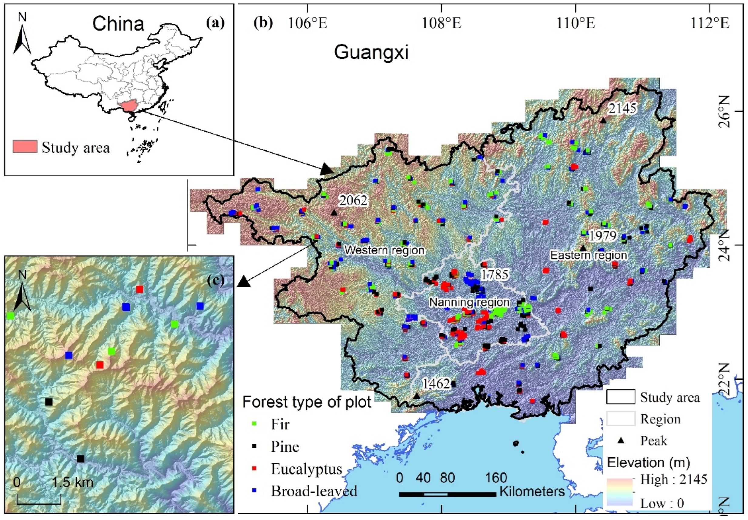
2.1. Study Site

The study area covered the entire Guangxi Zhuang Autonomous Region (104°28′–112°04′ E, 20°54′–26°24′ N) in southern China, with an area of 237.6 × 10³ km2 (Figure 1). In this study, airborne LiDAR data acquisition and field plot measurements were performed over three years in three regions based on financial allocations: the Nanning region (with an area of 22.1 × 10³ km2), the eastern region (128.4 × 10³ km2), and the western region (87.1 × 10³ km2).
Various landforms, such as mountains, hills, platforms, and plains, are distributed alternately in the study area, accounting for 62.1%, 14.5%, 9.1%, and 14.3% of the total land area, respectively. The topography is high in the northwest and low in the southeast, and the study area appears to be tilted from north and northwest to south and southeast. It is surrounded by mountains and plateaus; the central and southern parts are hilly with platforms and plains, forming the shape of a basin, which is known as the “Guangxi basin”. The highest elevation above sea level is 2145 m. The Tropic of Cancer crosses the central part of the study area, while the southern part borders a tropical ocean, and the study area is in the subtropical monsoon climate zone. In 2016, the mean annual temperature around the study area was 17.6–23.8 °C, and the mean annual temperature of the whole region was 21.4 °C. The total annual rainfall ranges from 723.9 to 2983.8 mm, with a region-wide mean annual rainfall of 1647.7 mm, including a region-wide average rainfall of 1234.4 mm during the flood season (April–September), accounting for 75% of the total annual rainfall.
From south to north, the study area comprises the northern tropics, southern subtropics, and central subtropics, and the representative forest vegetation is the seasonal rainforests, monsoon broad-leaved evergreen forests, and typical evergreen broad-leaved forests, respectively. The coniferous and bamboo forests are scattered in each vegetation zone. The Karst landscapes are widely distributed in the study area, with natural forests mainly including limestone (Rocky Mountain) monsoon forests, limestone mixed evergreen and deciduous broad-leaved forests, and limestone deciduous broad-leaved forests.
According to the 5th Forest Management Inventory of Guangxi (2017–2020), the forest area in the study area was 11,741.0 × 103 ha, accounting for 49.4% of the total land area, of which the Chinese fir (Cunninghamia lanceolata) planted forests, pine forests, eucalyptus plantations, and broad-leaved forests accounted for 16.5%, 17.5%, 24.8%, and 41.2% of the total forest area, respectively. The pine forests are mainly natural Pinus massoniana forests, with a few natural stands of P. yunnanensis var. tenuifolia and a small area of planted P. massoniana and P. elliottii forests. Industrial Eucalyptus spp. plantations are intensively managed plantations with a short rotation (5–8 years). The broad-leaved forests are multi-storied mixed forests composed of numerous tree species.

2.2. Field Plot Data

The field plots in the Nanning, eastern, and western regions were measured from October 2016 to January 2017, November 2018 to May 2019, and August 2019 to January 2020, respectively. The forests in the study area were categorized into four types: Chinese fir, pine, eucalyptus, and broad-leaved forest. The field plots were installed in the forest resources database in 2015 using ArcGIS Desktop v10.2 (ESRI, Redlands, CA, USA) based on the representativeness of the forest attributes, such as the mean height and stand volume. Approximately 100 plots were installed for each forest type in each region. The plots were distributed in clusters. The minimum spatial interval between the sample plots was 500 m (200 m in the Nanning region). There were 107 clusters of plots, each with 5–30 field plots (Figure 1). A hand-held dual-frequency differential global positioning system (GPS) was used to navigate to the stand on which the plot was located. The rectangular plot size was 30 × 20 m, all set in a north–south orientation, and was subdivided into four subplots each with a size of 15 × 10 m. The boundaries of the plot and subplots were measured and set using a compass and a handheld laser rangefinder and marked by nylon ropes. The Trimble GNSS (Global Navigation Satellite System) receiver with a real-time kinematic (RTK) positioning method was employed to position the northwestern and southeastern corners of the plot. Two RTK-GNSS instruments were used as the base stations, which were located in a nearby open field. Using the post-correction approach, the positioning accuracy was better than 1 m.
All live trees in each subplot with a DBH (1.3 m above the ground) greater than or equal to 5.0 cm were measured using a steel tape and identified by species or species groups. Three trees of average height and the tallest tree were selected to measure tree height with a Haglöf Vertex Ⅳ hypsometer. The calculation attributes of the subplots included the mean square diameter, mean height, basal area, stand volume, and stem density. The provincial species-specific allometric equations based on the basal area and mean height [49] were used to calculate the stand volumes. This study focused on the compatible models for estimating the stand attributes of pure forests. A stand is generally assumed to be a pure forest stand if the stems of the dominant species account for 80% of the total stem number. As the species (species group)-specific allometric equations were used to calculate the stand volume, we specified in this study that a forest stand was a pure forest stand only if the stand volume of the dominant species accounted for 95% of the total volume. The following methods were used to calculate the stand attributes of the field plots: The basal areas (G) of the four subplots were summed to obtain the basal area of the plots; the mean diameter (D) and mean height (H) of the plots were obtained from the weighted average of the basal areas of the subplots. The species (group)-specific allometric equations for calculating the stand volume (V) are as follows [49]:
V Fir = G × H × ( 0.4523 + 1.3133 H + 2 )
V Pine = G × H × ( 0.3645 + 1.9427 H + 2 )
V Eucalyptus = 0.9767 × G × D 0.06843 × H 0.8140
V Broadleaf = G × H × ( 0.4049 + 3.3787 H + 20 )
Since the stand volumes of the broad-leaved forests were calculated using the same allometric equation and were not divided into stand layers during the field measurement, all mixed broad-leaved stands were treated as pure forests. There were 782 pure forest field plots in the study area; the basic statistics of these plots are shown in Table 1.

2.3. LiDAR Data

LiDAR data were collected by several contractors from October 2016 to April 2017, October 2018 to October 2019, and August 2019 to January 2020 in Nanning, eastern, and western regions. The Riegl VQ−1560 and Riegl VQ−1560i laser scanning systems (Riegl Laser Measurement Systems GmbH: Horn, Austria) were applied to collect LiDAR data in all three regions with identical standards. The pulse repetition frequency of the laser scanner was 1000 kHz, the scan frequency was 146 Hz, and the maximum scan zenith angle was ±30°. The beam divergence was 0.50 mrad with an average footprint size of approximately 0.5 m. The relative aircraft flight altitude was approximately 2500 m, the flight speed was 200–240 km h−1, the swath width was 1.3–2.2 km, and the overlap between adjacent swathes was 21%–25%. The final average point density was ≥2.0 points m−2. The point clouds were geo-referenced to a projection system of the China Geodetic Coordinate System 2000 (CGCS2000).
Before being delivered to the end-users, the raw data were preprocessed by the contractors using TerraScan software (TerraSolid, Ltd., Helsinki, Finland). The echo signals were classified as ground returns or nonground returns using the adaptive triangulation network (TIN) filter algorithm. A digital terrain model (DTM) with grid cells of 2 m was generated using the ground returns. Then, we eliminate the effect of topography and obtain the DTM-normalized LiDAR point clouds using the DTM.
LiDAR-derived metrics were extracted using all the echoes of the normalized point clouds, including the mean (Hmean), standard deviation (Hstdev), and coefficient of variation (Hcv) of the point cloud distribution, the 95th height percentile (hp95); canopy closure (CC), and the 50th and 75th density percentiles (dp50 and dp75). In addition, to characterize the canopy vertical heterogeneity and understory vegetation within the stand, the leaf area density (LAD) profiles and vertical foliage profile (VFP)-related metrics were extracted from the LiDAR point clouds, which include the mean (LADmean), standard deviation (LADstdev), and coefficient of variation (LADcv) of LAD following Bouvier et al. [28], and the mean (VFPmean), standard deviation (VFPstdev), and coefficient of variation (VFPcv) of VFP following Harding et al. [50]. The LiDAR-derived metrics used in this study are shown in Table 2.

2.4. Independence Model

Forest attributes are closely related to the 3D structures of their canopies. The LiDAR point clouds can accurately depict the 3D structures of forest canopies [26,36,51]. The above 13 variables can be divided into three groups: height, density, and vertical structure variable groups. Then, the independent model (IM) of forest attribute estimation can be separately established by the multiplicative power model, and the model structure formulation is as follows [52]:
y ^ = a 0 P a 1 H a 2 S a 3 + ε
where y ^ is the estimate of the stand attribute (V, H, G, and D); P , H , and S are a group of LiDAR-derived variables depicting the canopy structure aspect of the density, height, and vertical structure, respectively, with each group containing 1–2 variables; and a 0 , a 1 , , a n are the parameters of the model.
To achieve a robust model for forest attribute estimation with good explanatory power, high accuracy, and conformity with the principles of forest mensuration and ecology, a multiplicative power model based on Equation (5) was constructed using a rule-based exhaustive combination method. One or two variables in each variable group were selected and include in Equation (5). A model formulation comprising 2–5 variables was obtained for a specific parameter of a specific forest type. The selection and combination of variables were performed according to the following rules:
(1)
The variable combination scheme: 1–2 height variables + 1–2 density variables +/1 vertical structure variable.
(2)
The model must comprise at least one primary height variable (Hmean or hp95) and one primary density variable (CC). When two height variables are selected, one primary and one secondary height variable (Hstdev or Hcv) can be included. When two density variables are selected, one secondary density variable is selected in addition to the CC.
(3)
Each variable in the group of vertical structure variables can appear in the model separately.
(4)
When the model comprises two variables, Equation (5) consists of one primary height variable and one primary density variable. When the model comprises three variables, Equation (5) consists of one primary height variable, one primary density variable, and one vertical structure variable. When the model comprises four variables, Equation (5) consists of one primary height variable, one secondary height variable, one primary density variable, and one vertical structure variable. When the model comprises five variables, Equation (5) consists of one primary height variable, one secondary height variable, one primary density variable, one secondary density variable, and one vertical structure variable.
Eighty-six model formulations were obtained using the above rule-based exhaustive combination approach, which was applicable to all forest attribute estimations of all forest types. To achieve the best forest type-specific model formulation for specific forest attribute estimation, each model formulation was subjected to fifty iterations of model calibration and validation using the field plot dataset of that forest type. For each iteration (using the Gauss–Newton algorithm), the model was calibrated using 80% of the samples selected randomly from the dataset and validated using the remaining 20%. After all 50 repeats had been completed, the mean rRMSE and mean R2 of that model formulation were calculated. Repeating the above procedures, we achieved the best model formulation with the smallest rRMSE and the largest R2 after traversing all 86 models.
All plots of the same forest type were used to calibrate the best model formulation, which was validated by a 10-fold cross-validation method to obtain the best model for the independent estimation of forest attributes.

2.5. Error-in-Variable Simultaneous Equations

From Equations (1)–(4), a forest attribute can be calculated with other attributes. In other words, there is an intrinsic mathematical relationship among the forest attributes. When they are estimated independently, the mathematical relationship among the estimates may not satisfy Equations (1)–(4) because of estimation errors. LiDAR variables can be used as exogenous variables to estimate two of the three stand attributes mentioned above (for the eucalyptus forests, three of the four attributes were estimated). The two (or three) attribute estimates can be used as endogenous variables to estimate the remaining stand attribute using Equations (1)–(4). As estimation errors exist in the forest attributes, the error-in-variable method (EIV) [47,53] was used to establish the simultaneous equations (SEq) for estimating the above forest attributes. The vector form of the multiple nonlinear error-in-variable SEq is:
{ f ( y i , x i , c ) = 0 Y i = y i + e i i = 1 , 2 , , n E ( e i ) = 0 , cov ( e i ) = σ 2 ψ
where x i is the measurement value of the q-dimensional error-out-variable; y i is the measurement value of the p-dimensional error-in-variable; f is the m-dimensional function; Y i is the unknown true value of y i ; the covariance matrix of the error is denoted as Φ = σ 2 Ψ , Ψ is the error structure matrix of e i , and σ 2 is the estimation error.
For the fir, pine, and broad-leaved forests, three SEqs were established, and for the eucalyptus forests, four SEqs were established. As an example, SEqs of the fir forests were as follows.
{ H ^ = a 0 i = 1 n x i a i + ε H G ^ = b 0 j = 1 m y j b j + ε G V ^ = b 0 j = 1 m y j b j × a 0 i = 1 n x i a i × ( 0.4523 + 1.3133 / ( a 0 i = 1 n x i a i + 2 ) ) + ε V
{ V ^ = c 0 k = 1 l z i c k + ε V H ^ = a 0 i = 1 n x i a i + ε H G ^ = c 0 k = 1 l z i c k / a 0 i = 1 n x i a i × ( 0.4523 + 1.3133 / ( a 0 i = 1 n x i a i + 2 ) ) + ε G
{ V ^ = c 0 k = 1 l z i c k + ε V G ^ = b 0 j = 1 m y j b j + ε G H ^ = c 0 k = 1 l z i c k / b 0 j = 1 m y j b j + ε H
Note: H and G are endogenous variables in SEquation (7); V and H are endogenous variables in SEquation (8); and V and G are endogenous variables in SEquation (9).
The terms x i ( i = 1 , 2 , , n ) , y j ( j = 1 , 2 , , m ) , and z k ( k = 1 , 2 , , l ) are the LiDAR-variables used to construct the prediction models of H, G, and V, respectively; the variables are the same as those used to in Equation (5); n , m and l are the number of LiDAR-variables; a 0 , a 1 , , a n , b 0 , b 1 , , b m , and c 0 , c 1 , , c l are the estimates of the model parameters; H ^ = 0.4523 H ^ × ( H ^ + 3.9036 ) / ( H ^ + 2 ) , once H ^ has been calculated via SEquation. (9), H ^ can be calculated; ε H , ε G , ε V and ε H are the residual errors of H, G, V, and H , respectively, and they all are assumed to obey a normal distribution with a mean of 0. SEquations (7)–(9) ensure that the mathematical relationships defined by Equation (1) are satisfied among the estimates of the fir forest attributes. The SEqs for the remaining forest types can be established by referring to the above method.
The parameter estimations of the SEq were performed using the nlssystemfit (nonlinear equation system estimation) function of R software version 3.6.1 [54]. The validating methods of the equations were the same as those described in Section 2.4.

3. Result

3.1. Performance of the Independence Model

Generally, the best independence models for all forest attribute estimations of all four forest types performed well. For the fir, pine, and eucalyptus forests, the rRMSEs of the stand volume (V) and mean height (H) prediction models were approximately 20% and 10%, respectively, and the rRMSE of the basal area (G) prediction models ranged from 15.77% to 19.71%. However, for the broad-leaved forests with a complex structure, the performances of all IMs were slightly worse, with the rRMSE of the V, H, and G prediction models being 31.41%, 15.74%, and 27.22%, respectively (Table 3). Overall, compared to the reported studies [13,21,24,28,55], and considering the large area and structural heterogeneity in this study area, we considered the performances of the IMs excellent.
A paired t-test was performed on V ^ I M i and V C i , and the results indicated that there were no statistically significant differences (α = 0.05) between the mean V ^ I M i and the mean V C i in the fir, pine, and broad-leaved forests, but there was statistically significant difference (α = 0.05) in the eucalyptus forests.

3.2. Performance of the Simultaneous Equations

The SEqs performed well for all four forest types. For the fir, pine, and eucalyptus forests, the variations in rRMSEs of the V, H, G, and D estimation were 16.16%–21.12%, 8.74%–10.74%, 15.80%–19.78%, and 11.69%–12.11%, respectively. For the broad-leaved forests, the rRMSEs of the V, H, and G estimations of the three SEqs were 30.92%–31.45%, 15.75%–15.99%, and 27.30%–27.369%, respectively (Table 3). The F-test results showed that the regression effects were statistically significant (α = 0.05) for all 43 equations in all 13 SEqs.
The differences in R2 and rRMSE were extremely small among different SEqs for the same attribute of the same forest type (Table 3). For example, in the pine forests, the differences between the largest and smallest values of R2 among the three SEqs for the V, H, and G estimations were 3.25%, 0.62%, and 3.62%, respectively. The relative differences between the largest and smallest values of rRMSE were 1.33%, 0.19%, and 3.39%, respectively. The differences in rRMSEs were less than 2.0% in over 80% of all 43 equations, with the largest being 5.85%, indicating that all the SEqs performed essentially the same and any two out of three forest attributes (four for eucalyptus forests) could be used as the endogenous variables to estimate another attribute in the SEqs without obvious differences in estimates. In addition, the R2 and rRMSE of the validation dataset for all attributes were relatively close to those of the calibration dataset for all SEqs, indicating that all the SEqs were quite robust. Based on the principle of the smallest rRMSE, the SEqs that used H and G as the endogenous variables to estimate V (SEq_V) in the fir, pine, and broad-leaved forests performed slightly better than the other two SEqs. In the eucalyptus forests, the SEq that used D, H, and V as the endogenous variables to estimate G (SEq_G) outperformed the three other SEqs.
The average differences in the estimates of the same attributes among the different SEqs were insignificant, not exceeding ±1.0% (Table 3). However, the variations in difference among the plots remained significant. Taking the fir forest as an example, the differences in H, G, and V between SEq_V and SEq_G varied between 2.25% and 1.09%, −9.76% and 4.17%, and −10.88% and 5.01%, respectively. Between SEq_V and SEq_H, the variations in the differences in H, G, and V were −12.69%–6.48%, −0.75%–6.68%, and −10.45%–5.15%, respectively (Figure 2).
The results of the paired t-test showed that there were no statistically significant differences (α = 0.05) in the means of the four forest attribute estimates between most of the SEqs in the fir, pine, and broadleaf forests. In the eucalyptus forests, there were statistically significant differences (α = 0.05) in the means estimates of D and G between the different SEqs. However, there were no statistically significant differences (α = 0.05) in H and V (Table 4).

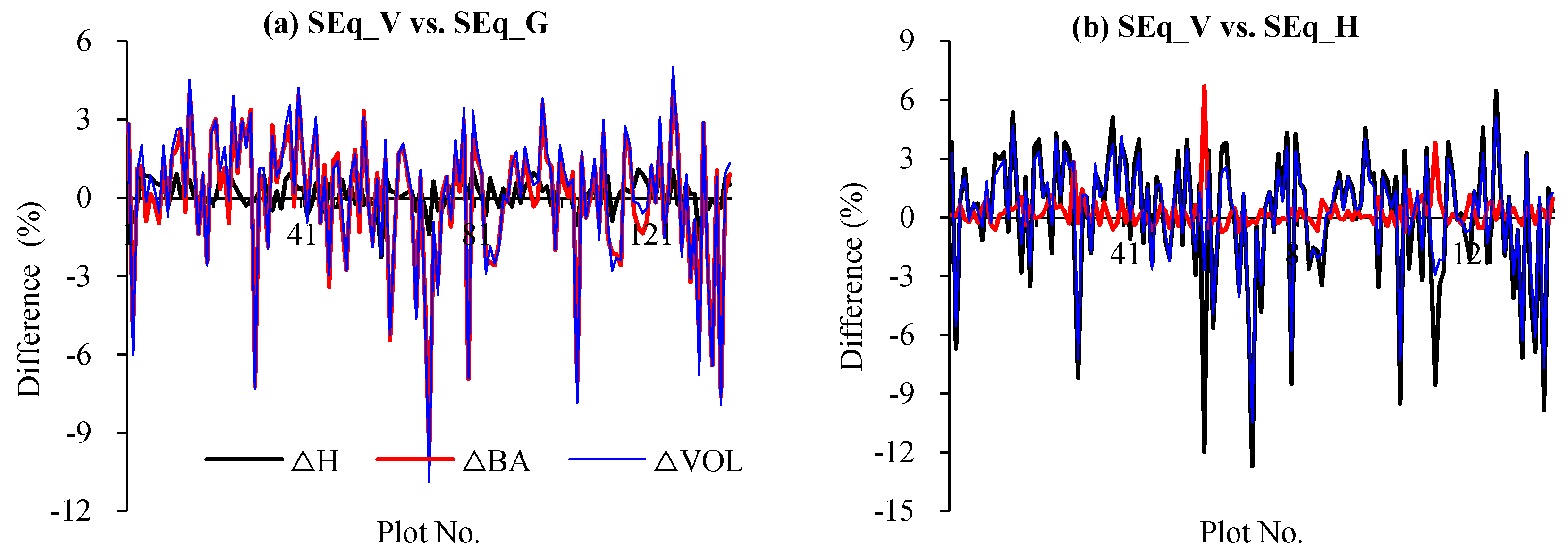
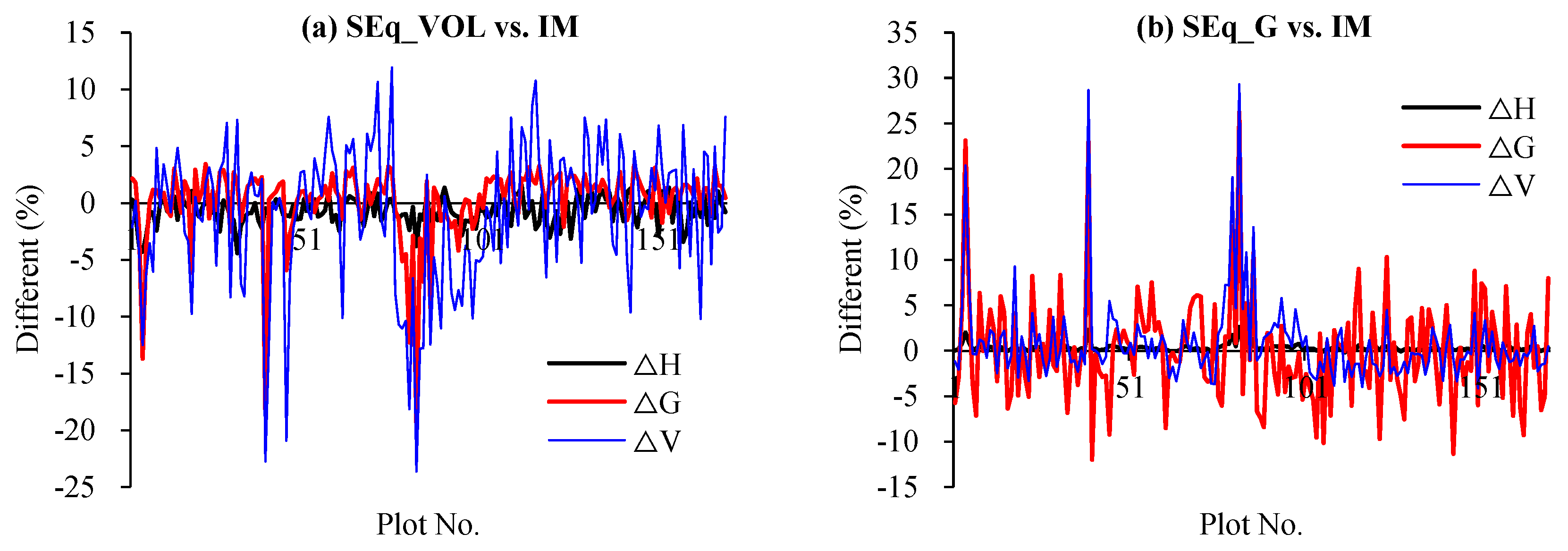
3.3. Comparison of the Simultaneous Equations and Independence Model

Compared to the IMs, the performances of the SEqs of all four forest types were slightly worse (Table 3). Although there were a few equations in the SEqs in which the R2 was larger and the rRMSE smaller than those of the IMs, the R2 of most SEqs was smaller than that of the IMs, and their rRMSE was larger than that of the IMs. The maximum decrease in R2 was −3.91%, and the maximum increase in rRMSE was 6.55%. Nevertheless, compared to the R2 and rRMSE of the IMs, over 90% of the equations in all 43 equations of all 13 SEqs showed that the decreases in R2 and the increases in rRMSE were not greater than 2%, indicating that the SEqs behaved similarly to the IMs.
Most of the average differences in the estimates between the SEqs and the corresponding IMs were less than ±1.0%, and the maximum average difference did not exceed ±2.0%, indicating that the estimates of the SEqs were close to those of the IMs. Nevertheless, the variations in the differences were large. For example, in the pine forests, the variations in the estimates of H, G, and V between the SEqs with H and G used as the endogenous variables (SEq_V) and the IMs were −4.40%–1.56%, −19.72%–3.44%, and −23.61%–11.94%, respectively; for the SEq_G, the variations in the estimates of the abovementioned attributes were −0.18%–2.62%, −11.98%–26.26%, and −4.09%–29.32%, respectively, as shown in Figure 3.
The results of the paired t-test of the estimates for all forest attributes of all forest types between the SEqs and the IMs showed that there were statistically significant differences (α = 0.05) in all attributes, except for the V of the pine forests (Table 5), despite the small average differences.
Although there were some differences in the estimates of forest attributes between the SEqs and IMs, and among the SEqs themselves, the estimations of all forest attributes of all forest types were good for both the IMs and SEqs (Figure 4).

4. Discussion

In this study, the error-in-variable simultaneous equation approach was used to construct estimation models of the mean stand height, mean stand diameter, basal area, and stand volume to achieve compatible estimates of forest attributes using airborne LiDAR data. The estimation methods were consistent with forest mensuration and ecology, and the mathematical consistencies were maintained among the estimates of forest attributes. Therefore, the presented approach is suitable for various estimation applications of the pure forest attributes and is useful for updating the forest resource database.
The estimation errors of all equations of the simultaneous equations were slightly larger than those of the independence models (Table 3). For the same attributes, although the average difference of the estimates between the simultaneous equations and the independence models was insignificant, not larger than 2%, there was a significant difference between their means (Table 5). The possible reasons were that during the iteration of SEq, the estimations of the forest attributes (such as H ^ and G ^ in SEquation (7)) using LiDAR variables as the endogenous variables were affected not only by their own errors but also by the errors of the attributes estimated using these variables as the endogenous variables (e.g., V ^ in SEquation (7)). In other words, the estimation errors of all forest attributes were treated synthetically during the calibration procedure of the simultaneous equations. Thus, the equation calibrations were subject to more constraints, which affected the estimation accuracy of all attributes to some extent.
The rRMSEs of the estimation equations for the same forest attribute were close among the SEqs (Table 3). There were few statistically significant differences between the estimates of the same stand attribute among the SEqs of the fir, pine, and broad-leaved forests (Table 4), indicating that the performances of different SEqs were very similar. There were statistically significant differences in the estimates of basal area and diameter at breast height among the simultaneous equations of the eucalyptus forests. The potential reason was that there were four equations in a SEq for the eucalyptus forest, one more than for the other forest types; therefore, the model calibration procedures were subjected to more constraints.
Equations (1)–(4) can be categorized into two classes: Equations (1), (2), and (4) belong to a class in which H and G are used as predictors to calculate V. Equation (3) belongs to another class in which V is calculated by H, D, and G. For the fir, pine, and broad-leaved forests, the SEqs that used H and G as the endogenous variables to estimate V performed slightly better than other SEqs, while the SEq that used DBH, H, and V as the endogenous variables for estimating G was the best in the eucalyptus forests (Table 3). The best SEqs were consistent with the classification of the allometric equations of the V calculations. This is possibly related to the estimation accuracy of all attributes in independent models. The estimation accuracy of V was lower than that of H, D, and G in all independent models for all forest types. Therefore, the best simultaneous equation was the one that estimated the remaining variables with the variables with the highest estimation accuracy as the exogenous variables.
A previous study proposed an allometric equation system to estimate stand attributes. This system estimated the key stand attributes, e.g., the stand volume and Lorey’s mean height, using LiDAR variables. Then, these two attributes were used directly to calculate G, QMD, and stand density (N, stems ha−1) using the allometric equations, which achieved good estimation results while maintaining compatibility among forest attributes [45]. In this study, we found that the differences between the V C directly calculated with H ^ I M , G ^ I M , and D ^ I M obtained from the IM based on Equations (1)–(4) and the V ^ I M obtained from the IM were small. There were no statistically significant differences, except in the eucalyptus forests. The average difference in V C and the estimate of stand volume ( V ^ S E ) obtained from the SEq was also small. However, there were statistically significant differences in their means in most of the equations. Furthermore, the estimation accuracy of other attributes strongly depended on the estimation accuracy of these two key attributes, and the stand volume was not a direct measurement predictor, indicating that the method also had some limitations. In this study, we found that the SEq using LiDAR variables as endogenous variables to estimate H and G, and then utilizing these two estimates as exogenous variables to estimate V, performed the best among several SEqs. Since H and G are directly measurable attributes in the field, these simultaneous equations can serve to boost the estimation accuracy.
In this study, we performed the compatible estimation of airborne LiDAR forest attributes by a multiplicative power model and error-in-variable simultaneous equations and achieved good results. However, the response of the same variable in different tree species is inconsistent. For instance, CC is positively correlated with H of fir, while it is negatively correlated with other tree species (Table 3). Additionally, there are numerous approaches to establishing prediction models of forest attributes using airborne LiDAR data, both parametric and nonparametric. There are various methods for establishing error-in-variable simultaneous equations. Therefore, more experiments are required to fully explore the performance of simultaneous equations in airborne LiDAR forest component attribute estimation.

5. Conclusions

In this paper, simultaneous equations (SEqs) were developed to estimate the mean stand height, mean diameter at breast height, basal area, and stand volume using airborne LiDAR data based on the measurement error model approach. The estimates were also analyzed and compared with the independence models (IMs). The following conclusions were drawn:
(1)
Both IMs and SEqs can achieve good estimation results for all forest parameters of all forest types. The SEqs performed slightly worse than the IMs; however, the difference was not obvious.
(2)
The SEqs maintain the definite mathematical relationships among various forest attributes, which are consistent with the principle of forest mensuration. The estimation results are useful for forest resource management.
(3)
For the Chinese fir, pine, and broad-leaved forests, the SEqs using the mean stand height, and basal area as the endogenous variables to estimate stand volume performed slightly better than the other two SEqs. For the eucalyptus forests, the SEqs with the diameter at breast height, mean stand height, and stand volume as the endogenous variables to estimate basal area (SEq_G) outperformed the other three SEqs.

Author Contributions

C.L.: conceptualization, methodology, calculation, data collection and analysis, writing—original draft and review and editing, project administration, funding acquisition. Z.Y. and X.Z.: Calculation and writing—original draft. M.Z. and Z.L.: Calculation. All authors have read and agreed to the published version of the manuscript.

Funding

This project received financial support from the Forest Department of Guangxi Zhuang Autonomous Region, China (GXLYKJ2016-001).

Data Availability Statement

The original data are available from the corresponding author.

Acknowledgments

This project is a part of the Fifth Forest Management Inventory Project of Guangxi Zhuang Autonomous Region (5th FMI-GX, 2017—2020), China. The airborne LiDAR data acquisition and preprocessing and field data measurement were funded by the finance department of the Guangxi Zhuang Autonomous Region. The authors would like to express their sincere gratitude to Chengling Yang and Yao Liang from the Guangxi Forest Inventory and Planning Institute (FIPI-GX) and to the 120 other field crews who worked on the field measurements. The authors also thank Guangxi 3D Remote Sensing Engineering Technology Co., Ltd., Feiyan Aero Remote Sensing Technology Co., Ltd., Zhongke Remote Sensing Technology Group Co., Ltd., and Guangzhou Jiantong Surveying and Mapping Geographic Information Technology Co., Ltd. These companies were responsible for the acquisition and preprocessing of the airborne LiDAR data utilized herein. We thank the anonymous reviewers and the editor for their insightful suggestions.

Conflicts of Interest

We declare that we have no financial and personal relationships with other people or organizations that could inappropriately influence our work, and that there is no professional or other personal interest of any nature or kind in any product, service and/or company that could be construed as influencing the position presented in, or the review of, this manuscript.

References

  1. FAO. Global Forest Resources Assessment 2020: Main Report; FAO: Rome, Italy, 2020. [Google Scholar] [CrossRef]
  2. Means, J.E.; Acker, S.A.; Fitt, B.J.; Renslow, M.; Emerson, L.; Hendrix, C.J. Predicting forest stand characteristics with airborne scanning lidar. Photogramm. Eng. Remote Sens. 2000, 66, 1367–1371. [Google Scholar]
  3. Torre-Tojal, L.; Bastarrika, A.; Boyano, A.; Lopez-Guede, J.M.; Graña, M. Above-ground biomass estimation from LiDAR data using random forest algorithms. J. Comput. Sci. 2022, 58, 101517. [Google Scholar] [CrossRef]
  4. Coops, N.C.; Tompalski, P.; Goodbody, T.R.; Queinnec, M.; Luther, J.E.; Bolton, D.K.; White, J.C.; Wulder, M.A.; van Lier, O.R.; Hermosilla, T. Modelling lidar-derived estimates of forest attributes over space and time: A review of approaches and future trends. Remote Sens. Environ. 2021, 260, 112477. [Google Scholar] [CrossRef]
  5. McRoberts, R.E.; Tomppo, E.O.; Næsset, E. Advances and emerging issues in national forest inventories. Scand. J. For. Res. 2010, 25, 368–381. [Google Scholar] [CrossRef]
  6. Johnson, K.D.; Birdsey, R.; Finley, A.O.; Swantaran, A.; Dubayah, R.; Wayson, C.; Riemann, R. Integrating forest inventory and analysis data into a LiDAR-based carbon monitoring system. Carbon Balance Manag. 2014, 9, 11. [Google Scholar] [CrossRef] [Green Version]
  7. Straub, C.; Tian, J.; Seitz, R.; Reinartz, P. Assessment of Cartosat-1 and WorldView-2 stereo imagery in combination with a LiDAR-DTM for timber volume estimation in a highly structured forest in Germany. Forestry 2013, 86, 463–473. [Google Scholar] [CrossRef] [Green Version]
  8. Mora, B.; Wulder, M.A.; White, J.C.; Hobart, G. Modeling stand height, volume, and biomass from very high spatial resolution satellite imagery and samples of airborne LiDAR. Remote Sens. 2013, 5, 2308–2326. [Google Scholar] [CrossRef] [Green Version]
  9. Fekety, P.A.; Falkowski, M.J.; Hudak, A. Temporal transferability of LiDAR-based imputation of forest inventory attributes. Can. J. For. Res. 2015, 45, 422–435. [Google Scholar] [CrossRef]
  10. Frank, B.; Mauro, F.; Temesgen, H. Model-based estimation of forest inventory attributes using Lidar: A comparison of the area-based and semi-individual tree crown approaches. Remote Sens. 2020, 12, 2525. [Google Scholar] [CrossRef]
  11. Asner, G.P.; Clark, J.K.; Mascaro, J.; Galindo García, G.A.; Chadwick, K.D.; Navarrete Encinales, D.A.; Paez-Acosta, G.; Cabrera Montenegro, E.; Kennedy-Bowdoin, T.; Duque, Á.; et al. High-resolution mapping of forest carbon stocks in the Colombian Amazon. Biogeosciences 2012, 9, 2683–2696. [Google Scholar] [CrossRef]
  12. Morsdorf, F.; Kötz, B.; Meier, E.; Itten, K.I.; Allgöwer, B. Estimation of LAI and fractional cover from small footprint airborne laser scanning data based on gap fraction. Remote Sens. Environ. 2006, 104, 50–61. [Google Scholar] [CrossRef]
  13. Naesset, E. Accuracy of forest inventory using airborne laser scanning: Evaluating the first nordic full-scale operational project. Scand. J. Res. 2004, 19, 554–557. [Google Scholar] [CrossRef]
  14. Næsset, E.; Gobakken, T.; Holmgren, J.; Hyyppä, H.; Hyyppä, J.; Maltamo, M.; Nilsson, M.; Olsson, H.; Persson, Å.; Söderman, U. Laser scanning of forest resources: The Nordic experience. Scand. J. Res. 2004, 19, 482–499. [Google Scholar] [CrossRef]
  15. White, J.C.; Tompalski, P.; Vastaranta, M.; Wulder, M.A.; Saarinen, N.; Stepper, C.; Coops, N.C. A Model Development and Application Guide for Generating an Enhanced Forest Inventory Using Airborne Laser Scanning Data and an Area-Based Approach; CWFC Information Report FI-X-018; Natural Resources Canada, Canadian Forest Service, Pacific Forestry Centre: Victoria, BC, Canada, 2017. [Google Scholar] [CrossRef]
  16. Næsset, E.; Bjerknes, K.-O. Estimating tree heights and number of stems in young forest stands using airborne laser scanner data. Remote Sens. Environ. 2001, 78, 328–340. [Google Scholar] [CrossRef]
  17. Næsset, E. Predicting forest stand characteristics with airborne scanning laser using a practical two-stage procedure and field data. Remote Sens. Environ. 2002, 80, 88–99. [Google Scholar] [CrossRef]
  18. Næesset, E.; Bollandsas, O.M.; Gobakken, T.; Gregoire, T.G.; Stahl, G. Model-assisted estimation of change in forest biomass over an 11 year period in a sample survey supported by airborne LiDAR: A case study with post-stratification to provide “activity data”. Remote Sens. Environ. 2013, 128, 299–314. [Google Scholar] [CrossRef] [Green Version]
  19. Packalén, P.; Maltamo, M. The k-MSN method for the prediction of species-specific stand attributes using airborne laser scanning and aerial photographs. Remote Sens. Environ. 2007, 109, 328–341. [Google Scholar] [CrossRef]
  20. Hudak, A.T.; Crookston, N.L.; Evans, J.S.; Hall, D.E.; Falkowski, M.J. Nearest neighbour imputation of species-level, plot-scale forest structure attributes from LiDAR data. Remote Sens. Environ. 2008, 112, 2232–2245. [Google Scholar] [CrossRef] [Green Version]
  21. Woods, M.; Pitt, D.; Penner, M.; Lim, K.; Nesbitt, D.; Etheridge, D.; Treitz, P. Operational implementation of a LiDAR inventory in Boreal Ontario. For. Chron. 2011, 87, 512–528. [Google Scholar] [CrossRef]
  22. Penner, M.; Pitt, D.G.; Woods, M.E. Parametric vs. nonparametric LiDAR models for operational forest inventory in Boreal Ontario. Can. J. Remote Sens. 2013, 39, 426–443. [Google Scholar] [CrossRef]
  23. Penner, M.; Woods, M.; Pitt, D. A comparison of airborne laser scanning and image point cloud derived tree size class distribution models in Boreal Ontario. Forests 2015, 6, 4034–4054. [Google Scholar] [CrossRef] [Green Version]
  24. Montealegre, A.L.; Lamelas, M.T.; de la Riva, J.A.; García-Martín, A.; Escribano, F. Use of low point density ALS data to estimate stand-level structural variables in Mediterranean Aleppo pine forest. Forestry 2016, 89, 373–382. [Google Scholar] [CrossRef] [Green Version]
  25. Zhang, Z.; Cao, L.; She, G. Estimating forest structural parameters using canopy metrics derived from airborne LiDAR data in subtropical forests. Remote Sens. 2017, 9, 940. [Google Scholar] [CrossRef] [Green Version]
  26. Xu, C.; Manley, B.; Morgenroth, J. Evaluation of modelling approaches in predicting forest volume and stand age for small-scale plantation forests in New Zealand with RapidEye and LiDAR. Int. J. Appl. Earth Obs. 2018, 73, 386–396. [Google Scholar] [CrossRef]
  27. Van Ewijk, K.; Treitz, P.; Woods, M.; Jones, T.; Caspersen, J. Forest site and type variability in ALS-based forest resource inventory attribute predictions over three Ontario forest sites. Forests 2019, 10, 226. [Google Scholar] [CrossRef] [Green Version]
  28. Bouvier, M.; Durrieu, S.; Fournier, R.A.; Renaud, J.P. Generalizing predictive models of forest inventory attributes using an area-based approach with airborne LiDAR data. Remote Sens. Environ. 2015, 156, 322–334. [Google Scholar] [CrossRef]
  29. Dube, T.; Siban, M.; Shoko, C.; Mutanga, O. Stand-volume estimation from multi-source data for coppiced and high forest Eucalyptus spp. silvicultural systems in Kwa Zulu-Natal, South Africa. ISPRS J. Photogram. 2017, 132, 162–169. [Google Scholar] [CrossRef]
  30. Giannico, V.; Lafortezza, R.; John, R.; Sanesi, G.; Pesola, L.; Chen, J. Estimating stand volume and above-ground biomass of urban forests using LiDAR. Remote Sens. 2016, 8, 339. [Google Scholar] [CrossRef] [Green Version]
  31. Yang, T.-R.; Kershaw, J.A., Jr.; Ducey, M.J. The development of allometric systems of equations for compatible area-based LiDAR-assisted estimation. Forestry 2021, 94, 36–53. [Google Scholar] [CrossRef]
  32. Asner, G.P.; Mascaro, J.; Muller-Landau, H.C.; Vieilledent, G.; Vaudry, R.; Rasamoelina, M.; Hall, J.S.; Van Breugel, M. A universal airborne LiDAR approach for tropical forest carbon mapping. Oecologia 2012, 168, 1147–1160. [Google Scholar] [CrossRef]
  33. Jenkins, J.C.; Chojnacky, D.C.; Heath, L.S.; Birdsey, R.A. National-scale biomass estimators for United States tree species. For. Sci. 2003, 49, 12–35. [Google Scholar]
  34. Hill, T.C.; Williams, M.; Bloom, A.A.; Mitchard, E.T.A.; Ryan, C.M. Are inventory based and remotely sensed above-ground biomass estimates consistent? PLoS ONE 2013, 8, e74170. [Google Scholar] [CrossRef] [Green Version]
  35. Sharma, M.; Oderwald, R.G. Dimensionally compatible volume and taper equations. Can. J. Res. 2001, 31, 797–803. [Google Scholar] [CrossRef]
  36. Buckman, R.E. Growth and Yield of Red Pine in Minnesota; Technical Bulletin 1272; USDA Forest Service: Washington, DC, USA, 1962; 50p, Available online: https://babel-hathitrust-org-s.vpn.gxu.edu.cn:8118/cgi/pt?id=uiug.30112019334355&view=1up&seq=3 (accessed on 10 May 2022).
  37. Clutter, J.L. Compatible growth and yield models for loblolly pine. For. Sci. 1963, 9, 354–371. [Google Scholar]
  38. Fang, Z.; Giley, R.L.; Shiver, B.D. A multivariate simultaneous prediction system for stand growth and yield with fixed and random effects. For. Sci. 2001, 47, 550–562. [Google Scholar]
  39. Wang, Y.; Huang, S.; Yang, R.C.; Tang, S. Error-in-variable method to estimate parameters for reciprocal base-age invariant site index models. Can. J. Res. 2004, 34, 1929–1937. [Google Scholar] [CrossRef]
  40. Fu, L.; Lei, Y.; Wang, G.; Bi, H.; Tang, S.; Song, X. Comparison of seemingly unrelated regressions with error-invariable models for developing a system of nonlinear additive biomass equations. Trees 2016, 30, 839–857. [Google Scholar] [CrossRef]
  41. Zhang, C.; Peng, D.-L.; Huang, G.-S.; Zeng, W.-S. Developing aboveground biomass equations Both compatible with tree volume equations and additive systems for single-trees in Poplar plantations in Jiangsu Province, China. Forests 2016, 7, 32. [Google Scholar] [CrossRef] [Green Version]
  42. Zeng, W.; Zhang, L.; Chen, X.; Cheng, Z.; Ma, K.; Li, Z. Construction of compatible and additive individual-tree biomass models for Pinus tabulaeformis in China. Can. J. Res. 2017, 47, 467–475. [Google Scholar] [CrossRef]
  43. Sakici, O.E.; Kucuk, O.; Ashraf, M.I. Compatible above-ground biomass equations and carbon stock estimation for small diameter Turkish pine (Pinus brutia Ten.). Environ. Monit. Assess 2018, 190, 285. [Google Scholar] [CrossRef]
  44. Fu, L.; Liu, Q.; Sun, H.; Wang, Q.; Li, Z.; Chen, E.; Pang, Y.; Song, X.; Wang, G. Development of a system of compatible individual tree diameter and aboveground biomass prediction models using error-in-variable regression and airborne LiDAR data. Remote Sens. 2018, 10, 325. [Google Scholar] [CrossRef] [Green Version]
  45. Yang, Z.; Liu, Q.; Luo, P.; Ye, Q.; Duan, G.; Sharma, R.P.; Zhang, H.; Wang, G.; Fu, L. Prediction of individual tree diameter and height to crown base using nonlinear simultaneous regression and airborne LiDAR data. Remote Sens. 2020, 12, 2238. [Google Scholar] [CrossRef]
  46. Kangas, A.S. Effect of errors-in-variables on coefficients of a growth model and on prediction of growth. For. Ecol. Manag. 1998, 102, 203–212. [Google Scholar] [CrossRef]
  47. Tang, S.; Li, Y.; Wang, Y. Simultaneous equations, error-in-variable models, and model integration in systems ecology. Ecol. Model. 2001, 142, 285–294. [Google Scholar] [CrossRef]
  48. Kinane, S.M.; Montes, C.R.; Albaugh, T.J.; Mishra, D.R. A model to estimate leaf area index in loblolly pine plantations using Landsat 5 and 7 images. Remote Sens. 2021, 13, 1140. [Google Scholar] [CrossRef]
  49. Liao, Z.; Huang, D. Forest Inventory Handbook of Guangxi, China; Forestry Department of Guangxi Zhuang Autonomous Region: Nanning, China, 1986. (In Chinese) [Google Scholar]
  50. Harding, D.J.; Lefsky, M.A.; Parker, G.G.; Blair, J.B. Laser altimeter canopy height profiles methods and validation for closed-canopy, broadleaf forests. Remote Sens. Environ. 2001, 76, 283–297. [Google Scholar] [CrossRef]
  51. Vauhkonen, J.; Maltamo, M.; McRoberts, R.E.; Næsset, E. Introduction to Forestry Applications of Airborne Laser Scanning. In Forestry Applications of Airborne Laser Scanning: Concepts and Case Studies; Managing Forest Ecosystems, 27; Maltamo, M., Næsset, E., Vauhkonen, J., Eds.; Springer: Dordrechtc, The Netherlands, 2014; Volume 464, pp. 1–18. [Google Scholar]
  52. Li, C.; Li, Z. Generalizing predictive models of sub-tropical forest inventory attributes using an area-based approach with airborne LiDAR data. Sci. Silvae Sin. 2021, 57, 23–35. (In Chinese) [Google Scholar] [CrossRef]
  53. Tang, S.; Wang, Y. A parameter estimation program for the errors-in-variable model. Ecol. Model. 2002, 156, 225–236. [Google Scholar] [CrossRef]
  54. R Core Team. R: A Language and Environment for Statistical Computing; R Foundation for Statistical Computing: Vienna, Austria, 2019; Available online: https://www.R-project.org/ (accessed on 20 August 2020).
  55. Zolkos, S.G.; Goetz, S.J.; Dubayah, R. A meta-analysis of terrestrial aboveground biomass estimation using lidar remote sensing. Remote Sens. Environ. 2013, 128, 289–298. [Google Scholar] [CrossRef]
Figure 1. Location of the study area. (a) Geographic location of study area in China; (b) distribution of field plots in three regions in study area; (c) locations of field plots.
Forests 14 00065 g001
Figure 2. The plot-level differences in the estimates of H, G, and V between the simultaneous equations of the fir forest: (a) SEq_V vs. SEq_G, (b) SEq_V vs. SEq_H.
Forests 14 00065 g002
Figure 3. The plot-level differences of the estimates of H, G, and V between the SEqs and the IMs of the pine forests: (a) H and G were used as the endogenous variables to estimate V; (b) H and V were used as the endogenous variables to estimate G.
Forests 14 00065 g003
Figure 4. Scatterplots of measured forest attributes vs. LiDAR-predicted forest attributes obtained from simultaneous equations and independence models (the solid line is the 1:1 line) of four forest types: (ac) fir forests; (df) pine forests; (gj) eucalyptus forests; (km) broad-leaved forests.
Forests 14 00065 g004
Table 1. Summary statistics of the field plot data. CV is the coefficient of variation.
Forest TypeSample SizeStem Density (Stems ha−1)Diameter at Breast Height (D)Stand Height (H)Basal Area (G)Stand Volume (V)
Mean (cm)CV (%)Mean (m)CV(%)Mean (m2ha−1)CV (%)Mean (m3ha−1)CV (%)
Fir139683–688311.826.210.6527.7633.3230.20205.6746.73
Pine170350–396719.528.014.3227.2628.5732.30206.9147.95
Eucalyptus267517–335011.221.416.1020.6317.1433.87141.1444.58
Broad-leaved206233–480013.634.510.4927.2519.2740.62110.1358.88
Table 2. List of LiDAR-derived metrics used in the establishment of the prediction model.
AcronymExplanation of MetricStructural AspectPredictor (Px)
HMean stand height (m)Target variable-
DDiameter at breast height (cm)Target variable-
VStand volume (m3 ha−1)Target variable-
GBasal area (m2 ha−1)Target variable-
HmeanMean height of point clouds (m)Canopy heightPhm
hp9595th height percentileCanopy heightPhm
HstdevStandard difference of point height distribution (m)Canopy heightPh
HcvCoefficient of variation of point height distributionCanopy heightPh
CCCanopy coverCanopy densityPdm
dp5050th density percentileCanopy densityPd
dp7575th density percentileCanopy densityPd
LADmeanMean of vertical leaf area density (LAD) profileVertical heterogeneityPv
LADstdevStandard difference of vertical LAD profileVertical heterogeneityPv
LADcvCoefficient of variation of vertical LAD profileVertical heterogeneityPv
VFPmeanMean of vertical foliage profile (VFP)Vertical heterogeneityPv
VFPstdevStandard difference of VFPVertical heterogeneityPv
VFPcvCoefficient of variation of VFPVertical heterogeneityPv
Table 3. The parameter estimates of the best independence models and simultaneous equations of varied forest types and their goodness-of-fit statistics.
Forest TypeModel TypeAttributeVariables and Their Parameter EstimatesFitting StatisticValidation Statistic
a0Hmeanhp95HstdevHcvCCdp50dp75LADmeanLADstdevLADcvVFPmeanVFPstdevVFPcvR2RMSE(%)R2RMSE(%)
FirIMV5.0365 1.2623 −0.35741.2661 0.03870 0.86715.960.85815.99
H1.4389 0.78970.02164 0.29020.08133 0.05820 0.85810.070.85010.08
G8.14600.7273 −0.1939 0.9878 0.03551 0.69215.860.67315.77
SEq_GV4.1305 1.2945 −0.39230.9746 0.04636 0.86316.210.85316.22
H1.3651 0.80400.005625 0.185200.06160 0.06417 0.85610.140.84710.14
G 0.68915.930.67115.80
SEq_VV 0.86416.140.85416.16
H1.4038 0.80160.01272 0.199100.06775 0.04897 0.85710.120.84810.13
G6.90210.7962 −0.2401 0.8014 0.04387 0.68516.030.66615.90
SEq_HV4.1094 1.2942 −0.39790.9664 0.04423 0.86316.220.85316.23
H 0.84010.700.82910.74
G7.01480.7866 −0.2254 0.8740 0.04492 0.68616.000.66715.87
PineIMV6.19821.4577 0.4028 −0.06050 0.82519.300.82419.01
H0.7293 1.0751 −0.01010 0.1209 0.8958.690.8898.73
G6.68660.7472 −0.04336 0.20110.3149 −0.10950.70217.250.70017.01
SEq_GV5.93871.4838 0.6551 −0.04736 0.82119.500.82119.14
H0.7407 1.0697 0.007975 0.1112 0.8948.700.8898.74
G 0.67518.020.67317.73
SEq_VV 0.83318.850.83218.53
H0.7596 1.0588 −0.01068 0.07242 0.8938.770.8878.80
G7.02950.7428 −0.03240 0.34900.3502 −0.11170.69717.390.69617.10
SEq_HV6.13861.4617 0.6392 −0.03340 0.82219.470.82219.11
H 0.8938.770.8888.78
G4.88150.8090 −0.08092 0.54780.1012 −0.012890.68917.630.68817.33
EucalyptusIMV5.6930 1.3300−0.01835 0.2280 0.3609 −0.1124 0.77720.990.76920.92
H2.0316 0.73290.006645 −0.1352 0.08831−0.01158 0.7649.950.7579.76
G2.9668 0.8470−0.05055 0.2734 0.2742 −0.1500 0.65719.830.65019.71
D1.5173 0.70180.04169 −0.1269 0.07403 −0.01798 0.69411.770.68311.62
SEq_GV4.6363 1.34310.007167 −0.003278 0.3653 −0.07611 0.77321.200.76521.12
H2.3845 0.66890.02462 −0.20860 0.1018−0.01090 0.76110.020.7559.85
G 0.65519.900.64919.77
D1.8010 0.63440.05877 −0.1909 0.08666 −0.01665 0.69111.830.68211.69
SEq_VV 0.77321.200.76521.12
H2.3393 0.67080.02836 −0.2194 0.1019−0.001516 0.75910.050.7539.89
G2.4802 0.8435−0.01378 0.1630 0.2884 −0.08184 0.65419.910.64819.78
D1.7722 0.63370.06019 −0.1975 0.08687 −0.009687 0.69011.850.68011.73
SEq_HV4.1199 1.36220.01500 0.008849 0.3622 −0.04535 0.77321.190.76521.11
H 0.75910.060.7539.90
G2.3542 0.8584−0.01386 0.1857 0.2851 −0.07427 0.65519.900.64919.77
D1.7558 0.63680.05998 −0.2179 0.08665 −0.01231 0.68911.860.68011.73
SEq_DV4.9610 1.32520.008399 −0.006183 0.3712 −0.08210 0.77321.200.76521.12
H2.3575 0.66780.02798 −0.2306 0.1033−0.002148 0.75910.060.7539.91
G2.6718 0.8236−0.01287 0.1580 0.2936 −0.08883 0.65419.910.64819.78
D 0.67112.200.66112.11
Broad-leavedIMV5.03401.2488 0.2287 0.07030 0.67831.380.66931.41
H2.26980.6531 −0.07921 0.09380 0.62015.760.61015.74
G3.74730.7143 0.4489 0.06407 0.50727.210.50127.22
SEq_GV4.50781.2782 0.2167 0.08187 0.67731.420.66731.45
H2.51170.6072 −0.08318 0.01247 0.61715.820.60615.80
G 0.48827.710.48327.69
SEq_VV 0.68830.910.67830.92
H2.13630.6785 −0.07103 0.11390 0.61915.780.60915.75
G3.12930.7583 0.3296 0.11350 0.49627.510.49227.46
SEq_HV4.51031.2779 0.2220 0.08284 0.67731.420.66731.45
H 0.60816.000.59815.99
G3.29120.7501 0.2817 0.07504 0.50327.320.49827.30
Note: IM was the independence model; for the fir, pine, and broad-leaved forest, SEq_V was the simultaneous equation in which H and G were endogenous variables to estimate V; SEq_G was the simultaneous equation in which H and V were endogenous variables to estimate G; SEq_H was the simultaneous equation in which V and G were endogenous variables to estimate H; the naming of the simultaneous equations for the eucalyptus forest was similar to above. Assuming that H ^ I M i , G ^ I M i , D ^ I M i , and V ^ I M i were the estimates of H, G, D, and V of plot I obtained by the IMs, respectively. By using Equations (1)–(4), we were able to calculate the stand volume ( V C i ) of plot i. The variations (means) of the difference ( ( V C i V ^ I M i ) ( V C i + V ^ I M i ) × 200 ) between V ^ I M i and V C i of the fir, pine, eucalyptus, and broad-leaved forests were −12.19%–4.95% (−0.03%), −14.25%–10.9% (−0.58%), −4.43%–8.86% (−0.20%), and −17.41%–8.68% (−0.27%), respectively. Although the mean differences between V ^ I M i and V C i were insignificant, the variations in the differences were large, and none of the differences were equal to 0. These results indicated that the independence estimates of H, D, G, and V were incompatible, i.e., they did not satisfy the mathematical relationship defined by Equations (1)–(4).
Table 4. Results of paired t-test of the mean stand attribute estimates for various forest types between the simultaneous equations.
Forest TypeEquation/Model for Comparison∆H∆G∆V∆D
Mean
(m)
Mean
(%)
Std.
(m)
Mean
(m2ha−1)
Mean
(%)
Std.
(m2ha−1)
Mean
(m3ha−1)
Mean
(%)
Std.
(m3ha−1)
Mean
(cm)
Mean
(%)
Std.
(cm)
FirSEq_V vs. SEq_G0.02 ***0.160.050.02 ns−0.050.730.54 ns0.094.58
SEq_V vs. SEq_H0.02 ns0.030.330.06 ***0.240.190.89 *0.284.57
SEq_G vs. SEq_H0.00 ns−0.120.310.04 ns0.290.750.35 ***0.190.53
PineSEq_V vs. SEq_D−0.02 *−0.360.150.08 ns0.191.380.47 ns−0.0710.17
SEq_V vs. SEq_H−0.04 ns−0.380.530.14 ns0.001.040.54 ns−0.2910.04
SEq_G vs. SEq_H−0.02 ns−0.020.530.06 ns−0.190.850.08 ns−0.221.28
Eucalyptus SEq_V vs. SEq_D0.01 ns0.080.090.00 ns−0.090.080.00 ns0.060.060.03 *−0.020.18
SEq_V vs. SEq_H0.00 ns−0.040.09−0.03 ***−0.090.070.00 *−0.050.04−0.25 ***−0.120.87
SEq_V vs. SEq_D0.00 ns−0.020.03−0.01 **−0.100.05−0.03 ns−0.310.29−0.03 ns−0.090.49
SEq_G vs. SEq_H−0.01 ns−0.120.12−0.03 ***0.000.12−0.01 **−0.110.06−0.28 ***−0.090.86
SEq_G vs. SEq_D−0.01 ns−0.100.10−0.01 ns−0.020.08−0.03 ns−0.380.30−0.06 *−0.070.41
SEq_H vs. SEq_D0.00 ns0.020.080.02 **−0.010.11−0.02 ns−0.270.260.22 **0.021.18
Broad-leavedSEq_V vs. SEq_D0.00 ns−0.010.17−0.03 ns−0.260.37−0.16 ns−0.273.59
SEq_V vs. SEq_H0.02 ns0.180.39−0.07 *−0.550.53−0.30 ns−0.393.56
SEq_G vs. SEq_H0.02 ns0.190.30−0.04 ns−0.290.51−0.13 ***−0.110.15
Note: * Significant at α = 0.05; ** Significant at α = 0.01; *** Significant at α = 0.001; ns, not significant (α > 0.05).
Table 5. Results of paired t-test of the mean stand attribute estimates for various forest types between the simultaneous equations and independence model.
Forest TypeEquation/Model for ComparisonSample Size∆H∆G∆V∆D
Mean
(m)
Mean
(%)
Std.
(m)
Mean
(m2 ha−1)
Mean
(%)
Std.
(m2ha−1)
Mean (m3ha−1)Mean
(%)
Std.
(m3ha−1)
Mean
(cm)
Mean
(%)
Std.
(cm)
FirSEq_G vs. IM1390.01 nc−0.270.12−0.43 ***1.340.95−1.88 ***1.165.42
SEq_V vs. IM 0.03 ***0.430.10−0.40 ***−1.390.68−1.34 **−1.077.13
SEq_H vs. IM 0.02 ns−0.390.39−0.46 ***1.630.53−2.23 ***1.355.46
PineSEq_G vs. IM166−0.04 ***0.330.04−0.11 ns0.041.26−0.82 ns0.876.23
SEq_V vs. IM −0.07 ***−0.690.130.15 **0.150.640.81 ns−0.949.35
SEq_H vs. IM −0.01 ns0.310.47−0.14 ns−0.151.05−0.54 ns0.655.90
EucalyptusSEq_G vs. IM2670.04 **0.440.21−0.11 ***−0.540.30−1.12 ***−0.424.120.04 ***0.540.14
SEq_V vs. IM 0.05 **0.520.25−0.12 ***−0.620.28−1.10 ***−0.454.090.04 ***0.600.17
SEq_H vs. IM 0.05 **0.560.28−0.09 ***−0.530.26−0.85 ***−0.334.090.05 ***0.650.18
SEq_D vs. IM 0.05 **0.270.27−0.11 ***−0.260.29−1.07 ***−0.184.110.07 **0.460.40
Broad-leavedSEq_G vs. IM206−0.03 ***0.410.14−0.14 *0.700.81−0.96 ***1.361.51
SEq_V vs. IM −0.03 ***−0.420.05−0.17 **−0.970.77−1.13 ***−1.644.00
SEq_H vs. IM −0.05 **0.600.37−0.10 **0.410.48−0.83 ***1.251.61
Note: * Significant at α = 0.05; ** Significant at α = 0.01; *** Significant at α = 0.001; ns, not significant (α > 0.05).
Disclaimer/Publisher’s Note: The statements, opinions and data contained in all publications are solely those of the individual author(s) and contributor(s) and not of MDPI and/or the editor(s). MDPI and/or the editor(s) disclaim responsibility for any injury to people or property resulting from any ideas, methods, instructions or products referred to in the content.

