Abstract
Tree mortality plays a vital role in the accuracy of growth and yield calculations. Economic loss caused by Heterobasidion sp. and Armillaria sp. is a common issue in forestry. Estonian forests, which are mostly managed, are susceptible to fungal infection due to freshly exposed wood surfaces, such as stumps and mechanical wounds. External signs of infection are often scarce and may lead to incorrect stand vitality valuation. Modern devices, such as the PiCUS 3 Sonic Tomograph, can be used for non-destructive decay assessment. We assessed decay in two intensively managed Norway spruce (Picea abies L. Karst.) stands in order to identify the reliability of sonic tomography in tree vitality assessment. We hypothesize that the tomograph assessment is more accurate than the visual assessment for detecting the extent of decay damage in Norway spruce stems. The sample trees were first visually assessed without additional equipment. In the second phase, the same sample trees were measured with the PiCUS 3 Sonic Tomograph. In the last part of the study, the sample trees were assessed from the tree stumps following the clear-cut. We identified a relationship (p-value < 0.001) between the tomograph assessment and the stump assessment when major decay was present. We did not discover a relationship between the visual assessment and stump assessment, indicating that evaluating the decay from external signs is inaccurate according to our results. Our data also indicate that the tomograph is not able to detect the early stages of decay damage, since it has no substantial effect on the wood structure.
1. Introduction
Tree mortality plays a critical role in forest development and function, but remains one of the least understood elements of growth and yield estimation [1,2,3]. In the early development of a young forest, a large number of individual trees will die due to competition [4]. As the tree is constantly growing, it always needs more resources and space to grow [5]. Continual competition, lack of nutrients, drought, air pollution, and a number of other circumstances often lead to a weakened tree, which makes it vulnerable to insect infestation, decay fungi, wind, and other factors [6,7]. In a natural hemiboreal forest, the majority of trees die due to competition or fungal infection, while wind has a lesser effect [8]. Heterobasidion sp. is a widespread forest pathogen in coniferous forests of the northern hemisphere [9,10]. Economic loss caused by fungus is a well-researched and well-known subject in forestry [11,12]. In Estonia, the most at-risk species are the second generation and older generation Norway spruce (Picea abies L. Karst.) stands growing on soils with a high lime content, Scots pine (Pinus sylvestris L.) stands growing on fresh and temporarily dry sandy soils [13], and Norway spruce stands which are growing on the fertile soils of former agricultural land [14]. As Estonian forests are mostly managed, each logging or management operation increases the opportunity for the stumps to become infected by Heterobasidion spores [13,15]. In managed forests, where stands are thinned, the chance of structural failure caused by wind is also more probable [16]. Freshly exposed wood surfaces, such as stumps and wounds on the roots or stems, are infected by basidiospores [17]. Once the primary infection is established within a stand, uninjured trees can also become infected by the vegetative growth of mycelium through root contacts or grafts [10]. Inter-tree competition should lead to an even spacing distribution of living and dead trees, but mortality caused by root rot (Armillaria sp. or Heterobasidion sp.) frequently results in the spatial clustering of dead trees [18]. In unevenly-aged managed Norway spruce stands, fungal genotype research suggests that overstory trees spread the infection to nearby growing younger spruces, and not vice versa [19]. The external indicators of stem and root decay are frequently hard to interpret, and the actual vitality of the tree is difficult to assess without felling the tree [20,21].
The number of tools and methods available for the nondestructive testing (NDT) for the purpose of tree examination has steadily grown in recent years [22,23,24]. A number of tests or techniques can be categorized as nondestructive, and a variety of tests can be performed [25,26,27,28]. These methods include different principles, such as mechanical, ultrasound, resonance, and acoustic tomography, and several others [27]. The use of modern devices, such as resistographs and sonic tomographs, show promising results compared to basic visual assessments [29,30,31,32,33]. Sonic tomography is based on the measurement of sound waves travelling through the tree trunk from one sensor to another. The sound waves required for the vitality assessment are caused by tapping with an electronic impact hammer [34]. The result of the measurement process is a tomogram illustrating the sound velocity distribution in the stem cross-section [35]. The velocity variance measured by the PiCUS 3 Sonic Tomograph is shown on a tomogram with pixels of different colors. The default and frequently used color code for interpreting the tomogram using the included software PiCUS Q74, Argus Electronic GmbH (Rostock, Germany) is as follows. Brown and black areas display fast velocities, which indicate healthy wood. Green pixels display medium velocities, indicating a transition area between solid and unsolid wood, but may also demonstrate problems inside the tree in some cases. Violet, blue, and white areas display decayed or hollow regions within the tree [36]. A processed sound velocity map (tomogram) can be used as a basis for making a scientific and knowledgeable decision about the vitality of the tree, without felling the tree [37]. However, this measurement is a time-consuming process, due to the complexity of the procedure for setting up the sensors and performing the series tapings in order to create sound waves [38].
Uncertainty regarding stand health may lead to inaccurate forest management decisions. Therefore, a more accurate method of decay evaluation in Estonia is needed. The aim of this research is to assess the viability of sound tomography in stand health evaluation. We hypothesize that the tomograph assessment is more accurate than the visual assessment for detecting the extent of decay damage in Norway spruce stems.
2. Materials and Methods
2.1. Research Area and Study Design
The study was conducted in two research areas (RA1 & RA2), which were established in middle-aged spruce stands dominated by Norway spruce (Table 1). Both stands were growing on fertile soil, associated with a higher probability of Heterobasidion sp. infection [39]. The stands were designated for sanitation harvest by local forest managers due to extensive bark stripping (moose damage). Moose damage can be associated with the spread of the fungus, but the stem and root wounds are not as essential for Heterobasidion sp. infection as freshly cut stumps [40,41]. A total of 50 sample trees were selected from the tract with a randomized path. The chosen sample trees were evaluated visually from a living tree using the PiCUS 3 Sonic Tomograph and visually from a tree stump after the clear-cut. Forest measurement equipment was used to obtain the supplementary information. In order to identify and compare the sample trees after the clear-cut (stump assessment), each sample tree was marked with a plastic number card bearing a unique number and painted with the corresponding color in sequence (red, green, blue, yellow and white). In addition, the azimuth and distance of the successive trees were recorded as a secondary measure in case of identification problems.

Table 1.
Research area characteristics and dendrometric parameters (stand inventory data from the Estonian forest registry) [42].
2.2. Visual Assessment
All sample trees were visually assessed in the first phase of the study, with no extra equipment. The Estonian Network of Forest Research Plots (ENFRP) measurement protocol was the basis for the visual assessment [45]. Bark stripping, cracks, cavities, cold and wind damage, fruiting bodies, resin flow, and other external visual signs were used to determine vitality (Figure 1). The trees were examined from all sides, from the stump to the crown. Visual assessment is qualitative in nature and tends to be biased according to the assessor’s experience, which should be considered when interpreting visual assessment results [31]. Of the 50 trees examined, 23 were classified as healthy, as no visible defects were recorded. The other 27 sample trees were classified according to the severity of the defect. The opening (pruning wound, crack, or cavity) in the tree provides access to the decay fungi, but the characteristics and size of the damage must be taken into account as the severity is determined [46]. Bark removal was the most frequently occurring external defect recorded, which is associated with the spread of decay fungi. Bark removal was recorded in 47% of the sample trees in the first study area and in 65% of the sample trees in the second study area. A picture of each sample tree was taken from four directions (north, south, west, and east).
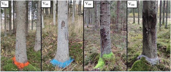
Figure 1.
Examples of visual assessment classes (healthy sample tree Vhy; sample tree with minor defect Vmi; sample tree with medium defect Vme; and sample tree with major defect Vma).
2.3. PiCUS 3 Sonic Tomograph Assessment
Sample trees were evaluated in the second phase of the study with the PiCUS 3 Sonic Tomograph, which functions by measuring the variation in the times that it takes the sound waves to travel between the measurement points across the trunk in order to determine patterns of wood integrity [36,37]. The pixel color spectrum (black, brown, green, violet, blue, and white) ranges from 100% velocity (brown) to the slowest velocity (blue) and is calculated with the principle of relative velocity, which is calibrated automatically at each measured cross-section [36]. In the first step, a compass was used to determine the northern direction, which was always the location of the first measurement point (a nail). The exact positions of the nails were used for the mapping, which enabled a more accurate comparison in the data analysis. The first nail was placed 30 cm above the ground, which was the measurement level used for all the tomograph measurements. The back of the first nail was always facing north. This height was chosen according to the stump cutting height provided by the local forest managers. Eight nails were used for each sample tree. All nails were placed roughly at same level around the tree. The geometry of the measuring level was calculated using the “Circular geometries” method. This method requires the circumference of the tree and the distances between the measuring points to be calculated. One tomogram was taken for each sample tree. The classification of the assessment was performed prior to the tomograph measurements in order to assess the tomograph sensitivity in the evaluation of the hidden decay of the Norway spruce. Tomograms with black and brown pixel percentages of 99%–100% were classified as healthy. This range was chosen due the “cog wheel effect”, which sometimes results in lower sonic velocity along the circumference, even when the algorithm is applied, but is not associated with decay or cavities [36]. Tomograms with black and brown pixel percentages of 95%–98% were classified as minor defect tomograms. Tomograms with black and brown pixel percentages of 91%–94% were classified as medium defect tomograms. Tomograms with black and brown pixel percentages of 90% or less were classified as major defect tomograms. The program PiCUS Q74 was used to study the tomograph assessment results after the measurements (pixel cloud distributions and location, and sonic wave travel speed). The cog wheel algorithm was applied before the final pixel calculation was carried out. Of the 50 tomograms, 38 were assigned as healthy (Figure 2). The other 12 tomograms were classified according to the solid wood percentage.
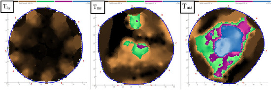
Figure 2.
Examples of tomograph assessment classes (healthy tomogram Thy; tomogram with medium defect Tme; and tomogram with major defect Tma) The numbers around the tomogram (1–8) indicate the location of the measurement points.
2.4. Tree Stump Assessment
All sample trees were assessed for decay after the clear-cut. The preliminary growth of the Heterobasidion sp. in the tree causes a color change in the wood, which indicates that the tree has been infected by a fungus [21,47]. Stumps with significant discoloration or other minor defects, which had no substantial effect on the structural stability, were categorized as slightly defective (minor defect). Stumps with a decay percentage less than half of the total volume of the stump were categorized as moderately defective (medium defect). Stumps with a decay percentage of more than half the total volume of the stump or extensive decay levels were categorized as severely defective (major defect). Of the 50 tree stumps examined, 26 were classified as healthy, as no visible defects in wood were recorded. The other 24 sample trees were classified according to the severity of the defect (Figure 3). Pictures were taken of each tree stump.
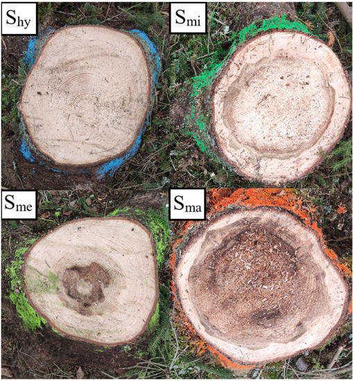
Figure 3.
Examples of stump assessment classes (healthy sample tree stump Shy; sample tree stump with minor defect Smi; sample tree stump with medium defect Sme; and sample tree stump with major defect Sma).
2.5. Data Analysis
All available data from the visual, tomograph, and stump assessments were used to compile the data table. The pixel percentages (high velocities Pbb, medium velocities Pg, low velocities Pvbw) of each sample tree from the PiCUS Q74 analysis were added to the data table. The visual, tomograph, and stump assessment data were used to form contingency tables. The Chi-squared test and Fisher’s exact test were used to compare the contingency tables (visual assessment to stump assessment and tomograph assessment to stump assessment). The Chi-squared test statistic and Fisher’s exact test are both used to evaluate whether there is a relationship between the rows and columns in a contingency table [48,49,50,51]. The contingency table was visualized as a mosaic diagram, which presents the distributions of the sample trees according to the decay severity and the assessment method capacity for detecting decayed and healthy trees [52]. The research areas (RA1 & RA2) were examined independently from one another to assess whether the results were different when the research areas were studied separately. Detached contingency tables were calculated for both research areas. The difference between research areas was visualized with a fourfold display, which is designed for 2 × 2 or 2 × 2 × k tables [52]. In order to evaluate the accuracy of the decay assessment using the different methods, five generalized linear models were calculated [53]. We compared the models using two different binary variables (stump with a major defect and a healthy stump, Table 2). The independent variables were: major defect assessed with the tomograph (model M1); major defect assessed visually (model M2); and major defect assessed with the tomograph + major defect assessed visually (model M3). The interval variables were the solid wood (black or brown pixel) percentage (model M4), and the decayed or hollow wood (violet, blue, and white pixel) percentage (model M5). The Akaike information criterion (AIC) was calculated for each model. The results were compared in order to validate the accuracy of the model estimates. All the calculations were made in R version 4.0.5 [54].
Table 2.
The generalized linear models (1–5) based on two different binary variables (stump with major defect and healthy stump). Acronym explanations are given in the materials and methods chapter.
3. Results
The Fisher’s exact and Chi-squared tests identified a relationship between major decay Tma (Pbb < 90%) assessed using the PiCUS 3 Sonic Tomograph and a severely decayed tree stump Sma (p-value < 0.001). We did not discover any relationship (p-value = 0.651) between a severely defective tree evaluated using a visual assessment Vma and a severely decayed tree stump Sma, indicating that assessing major decay from the external signs is inaccurate, based on our data. We found a relationship (p-value < 0.001) between the tomograph assessment Thy and the stump assessment Shy when a healthy tree was assessed, suggesting that the tomograph does not define healthy trees as severely decayed. There was no relationship between the visual assessment Vhy and stump assessment Shy when the healthy tree was assessed (p-value < 0.382), which implies that a tree which appears healthy from its external signs might actually be decayed (Table 3; Figure 4).
Table 3.
Fisher’s exact and chi-squared test results based on the contingency table (visual assessment to stump assessment and tomograph assessment to stump assessment). Acronym explanations are given in the materials and methods chapter.
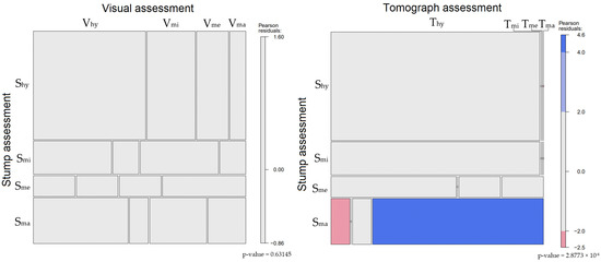
Figure 4.
Classification of sample trees according to decay assessment method and the association between the results obtained using the various methods: (left) comparison between the visual assessment and stump assessment; (right) comparison between the tomograph assessment and stump assessment. Blue color indicates that there are more observations in the cell than would be expected under the null model (independence). Red means that the cells show less than the expected frequency of observations [52]. Acronym explanations are given in the materials and methods chapter.
The research area parameters (RA1 & RA2) were found not be significant according to our data (Figure 5).
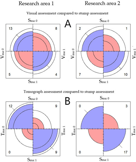
Figure 5.
Comparison between the two research areas. (A) The relationship between major defect assessed visually Vma and major defect assessed from the tree stump Sma. (B) The relationship between major defect assessed with the tomograph Tma and major defect assessed from the tree stump Sma. The relationship between variables is indicated by the tendency of the diagonally located cells. Color is used to indicate direction [52].
4. Discussion
The use and viability of modern devices have grown over the years, but visual assessment has been and continues to be an important part of tree defect evaluation [55]. Innovative methods, such as sound tomography (PiCUS 3 Sonic Tomograph), can be used for the non-invasive analysis of the internal structure of the tree trunk without damaging the tree, but there are limitations to this method [37]. The tomogram is limited to a specific cross-sectional area that does not represent the entire length of the tree and does not account for all the other factors which might affect tree vitality [27,56]. In order to produce an accurate tomogram, it is essential to position the sensors correctly and to measure correctly the distance between them [57]. In a forest, it is often desirable to use fewer sensors because of limited time, which affects the accuracy of the tomogram [38]. Our study findings correlate with those of other studies, as the tomograph estimated the proportion of the decay in the living tree to be lower than it was when evaluated from the stump assessment [30,56,58]. The PiCUS 3 Sonic Tomograph was able to identify trees with major decay in almost all cases, but there was one exception, which may have been caused by a technical problem or measurement error. The healthy wood pixel percentage of the given tomogram was 99%, but the location of the green pixel was irregular. The green pixels were in the middle, not at the edge, of the tomograph, as occurs frequently due to the cogwheel effect. This dissymmetry reinforces the fact that different aspects of the tomogram and tree should be considered, in addition to the pixel percentage, before determining the vitality of the tree.
Discoloration or the initial stages of decay are not shown in tomograms, according to our data, and therefore the use of fewer classes for tomograph assessments is advised. This issue was also pointed out in research about incipient decay in tree stems [59]. Our data suggests that visual defects, such as extensive moose damage, in a stand may not always indicate fungus infection. Only the first research area was moderately affected by decay fungus, while both research areas had similar levels of moose damage. The variance between the research areas may have been influenced by the fact that there was a previous clear-cut next to the first research area. This difference may have also been affected to some extent by the fact that the external defects were usually at a higher level compared to the tomography measurements, which were measured at 30 cm from the ground. Therefore, the trees could have also been affected by fungus at a higher level.
5. Conclusions
We identified a relationship between the tomograph assessment and stump assessment of decay when a major defect was present, indicating that the tomograph is more accurate than visual assessment when assessing heavily decayed trees. We did not discover a relationship between the visual assessment and stump assessment, indicating that evaluating decay from external signs is not accurate. The tomograph was not able to detect early stages of decay, which have no meaningful effect on the wood structure. These results suggest that sonic tomography can be used as a reliable method for assessing major decay within the Norway spruce stands. The obtained information about the tomograph viability, accuracy, and limits will be used in future research whose main objective is to study the extent of hidden decay in Estonian forests.
Author Contributions
Conceptualization D.L., A.K. and T.T.; methodology, D.L., A.K. and T.T.; software, T.T.; validation, T.T.; formal analysis, T.T. and A.K.; investigation, T.T. and A.N.; resources, T.T. and A.N.; data curation, T.T.; writing—original draft preparation, T.T.; writing—review and editing, D.L., A.K. and A.S.; visualization, T.T. and A.K.; supervision, D.L. and A.K.; project administration, D.L.; funding acquisition, D.L. All authors have read and agreed to the published version of the manuscript.
Funding
This research received no external funding.
Data Availability Statement
Data are available from the corresponding author upon reasonable inquiry.
Acknowledgments
We would like to thank the reviewers for their thoughtful comments and efforts towards improving our manuscript.
Conflicts of Interest
The authors declare no conflict of interest. The funders had no role in the design of the study; in the collection, analyses, or interpretation of data; in the writing of the manuscript; or in the decision to publish the results.
References
- Bertini, G.; Ferretti, F.; Fabbio, G.; Raddi, S.; Magnani, F. Quantifying Tree and Volume Mortality in Italian Forests. For. Ecol. Manag. 2019, 444, 42–49. [Google Scholar] [CrossRef]
- Adame, P.; Del Río, M.; Cañellas, I. Modeling Individual-Tree Mortality in Pyrenean Oak (Quercus pyrenaica Willd.) Stands. Ann. For. Sci. 2010, 67, 810. [Google Scholar] [CrossRef]
- Monserud, R.A.; Sterba, H. Modeling Individual Tree Mortality for Austrian Forest Species. For. Ecol. Manag. 1999, 113, 109–123. [Google Scholar] [CrossRef]
- Peet, R.K.; Christensen, N.L. Competition and Tree Death. BioScience 1987, 37, 586–595. [Google Scholar] [CrossRef]
- Pretzsch, H. Forest Dynamics, Growth and Yield: From Measurement to Model; Springer: Berlin/Heidelberg, Germany, 2010; ISBN 9783540883067. [Google Scholar]
- Negi, J.D.S.; Chauhan, P.S. Tree Mortality: Assesment and Mitigation; Scientific Publisher: Jodhpur, India, 2017. [Google Scholar]
- Kuuluvainen, T.; Aakala, T. Natural Forest Dynamics in Boreal Fennoscandia: A Review and Classification. Silva Fenn. 2011, 45, 823–841. [Google Scholar] [CrossRef]
- Laarmann, D.; Korjus, H.; Sims, A.; Stanturf, J.A.; Kiviste, A.; Köster, K. Analysis of Forest Naturalness and Tree Mortality Patterns in Estonia. For. Ecol. Manag. 2009, 258, S187–S195. [Google Scholar] [CrossRef]
- Otrosina, W.J.; Garbelotto, M. Heterobasidion occidentale Sp. Nov. and Heterobasidion irregulare Nom. Nov.: A Disposition of North American Heterobasidion Biological Species. Fungal Biol. 2010, 114, 16–25. [Google Scholar] [CrossRef]
- Garbelotto, M.; Gonthier, P. Biology, Epidemiology, and Control of Heterobasidion Species Worldwide. Annu. Rev. Phytopathol. 2013, 51, 39–59. [Google Scholar] [CrossRef]
- Gonthier, P.; Brun, F.; Lione, G.; Nicolotti, G. Modelling the Incidence of Heterobasidion annosum Butt Rots and Related Economic Losses in Alpine Mixed Naturally Regenerated Forests of Northern Italy. For. Pathol. 2012, 42, 57–68. [Google Scholar] [CrossRef]
- Woodward, S. Heterobasidion annosum: Biology, Ecology, Impact, and Control. Plant Pathol. 1998, 48, 564–565. [Google Scholar]
- Hanso, S.; Hanso, M. Spread of Heterobasidion annosum in Forests of Estonia. Metsanduslikud Uurim. 1999, XXXI, 162–172. [Google Scholar]
- Sierota, Z. Heterobasidion Root Rot in Forests on Former Agricultural Lands in Poland: Scale of Threat and Prevention. Sci. Res. Essays 2013, 8, 2298–2305. [Google Scholar]
- Piri, T.; Korhonen, K. The Effect of Winter Thinning on the Spread of Heterobasidion parviporum in Norway Spruce Stands. Can. J. For. Res. 2008, 38, 2589–2595. [Google Scholar] [CrossRef]
- Hallinger, M.; Johansson, V.; Schmalholz, M.; Sjöberg, S.; Ranius, T. Factors Driving Tree Mortality in Retained Forest Fragments. For. Ecol. Manag. 2016, 368, 163–172. [Google Scholar] [CrossRef]
- Asiegbu, F.O.; Adomas, A.; Stenlid, J. Conifer Root and Butt Rot Caused by Heterobasidion annosum (Fr.) Bref. s.l. Mol. Plant Pathol. 2005, 6, 395–409. [Google Scholar] [CrossRef]
- Dobbertin, M.; Baltensweiler, A.; Rigling, D. Tree Mortality in an Unmanaged Mountain Pine (Pinus Mugo Var. Uncinata) Stand in the Swiss National Park Impacted by Root Rot Fungi. For. Ecol. Manag. 2001, 145, 79–89. [Google Scholar] [CrossRef]
- Piri, T.; Valkonen, S. Incidence and Spread of Heterobasidion Root Rot in Uneven-Aged Norway Spruce Stands. Can. J. For. Res. 2013, 43, 872–877. [Google Scholar] [CrossRef]
- Liu, L.; Li, G. Acoustic Tomography Based on Hybrid Wave Propagation Model for Tree Decay Detection. Comput. Electron. Agric. 2018, 151, 276–285. [Google Scholar] [CrossRef]
- Heineman, K.D.; Russo, S.E.; Baillie, I.C.; Mamit, J.D.; Chai, P.P.-K.; Chai, L.; Hindley, E.W.; Lau, B.-T.; Tan, S.; Ashton, P.S. Evaluation of Stem Rot in 339 Bornean Tree Species: Implications of Size, Taxonomy, and Soil-Related Variation for Aboveground Biomass Estimates. Biogeosciences 2015, 12, 5735–5751. [Google Scholar] [CrossRef]
- Proto, A.R.; Cataldo, M.F.; Costa, C.; Papandrea, S.F.; Zimbalatti, G. A Tomographic Approach to Assessing the Possibility of Ring Shake Presence in Standing Chestnut Trees. Eur. J. Wood Wood Prod. 2020, 78, 1137–1148. [Google Scholar] [CrossRef]
- van Wassenaer, P.; Richardson, M. A Review of Tree Risk Assessment Using Minimally Invasive Technologies and Two Case Studies. Arboric. J. 2009, 32, 275–292. [Google Scholar] [CrossRef]
- Zhang, J.; Khoshelham, K. 3D Reconstruction of Internal Wood Decay Using Photogrammetry and Sonic Tomography. Photogramm. Rec. 2020, 35, 357–374. [Google Scholar] [CrossRef]
- Gao, S.; Wang, X.; Wiemann, M.; Brashaw, B.; Ross, R.; Wang, L. A Critical Analysis of Methods for Rapid and Nondestructive Determination of Wood Density in Standing Trees. Ann. For. Sci. 2017, 74, 27. [Google Scholar] [CrossRef]
- Ross, R.J. Nondestructive Evaluation of Wood: Second Edition; USDA Forest Service, Forest Products Laboratory, General Technical Report FPL-GTR-238; USDA Forest Service, Forest Products Laboratory: Washington, DC, USA, 2015; 176p. [Google Scholar]
- Brashaw, B.; Bucur, V.; Gonçalves, R.; Lu, J.; Meder, R.; Pellerin, R.; Potter, S.; Ross, R.; Wang, X.; Yin, Y. Nondestructive Testing and Evaluation of Wood: A Worldwide Research Update. For. Prod. J. 2009, 59, 7–14. [Google Scholar]
- Wang, X.; Pilon, C.; Brashaw, B.; Ross, R.; Pellerin, R. Assessment of Decay in Standing Timber Using Stress Wave Timing Nondestructive Evaluation Tools: A Guide for Use and Interpretation; U.S. Department of Agriculture, Forest Service: Washington, DC, USA, 2011. [Google Scholar]
- Allikmäe, E.; Laarmann, D.; Korjus, H. Vitality Assessment of Visually Healthy Trees in Estonia. Forests 2017, 8, 223. [Google Scholar] [CrossRef]
- Burcham, D.C.; Brazee, N.J.; Marra, R.E.; Kane, B. Can Sonic Tomography Predict Loss in Load-Bearing Capacity for Trees with Internal Defects? A Comparison of Sonic Tomograms with Destructive Measurements. Trees—Struct. Funct. 2019, 33, 681–695. [Google Scholar] [CrossRef]
- Koeser, A.K.; Hauer, R.J.; Klein, R.W.; Miesbauer, J.W. Assessment of Likelihood of Failure Using Limited Visual, Basic, and Advanced Assessment Techniques. Urban For. Urban Green. 2017, 24, 71–79. [Google Scholar] [CrossRef]
- Lavrov, M.F.; Doktorov, I.A.; Parnikova, G.M. Creation of Density Distribution Charts in the Cross and Axial Section of a Tree Trunk—Short Communication. J. For. Sci. 2016, 62, 571–579. [Google Scholar] [CrossRef]
- Qiu, Q.; Qin, R.; Lam, J.H.M.; Tang, A.M.C.; Leung, M.W.K.; Lau, D. An Innovative Tomographic Technique Integrated with Acoustic-Laser Approach for Detecting Defects in Tree Trunk. Comput. Electron. Agric. 2019, 156, 129–137. [Google Scholar] [CrossRef]
- Rust, S. Comparison of Methods to Measure Sensor Positions for Tomography. Arboric. J. 2020, 43, 180–186. [Google Scholar] [CrossRef]
- Baláš, M.; Gallo, J.; Kuneš, I. Work Sampling and Work Process Optimization in Sonic and Electrical Resistance Tree Tomography. J. For. Sci. 2020, 66, 9–21. [Google Scholar] [CrossRef]
- Göcke, L. PiCUS Sonic Tomograph Manual of PC Software Q74. 2017. Available online: http://www.argus-electronic.de/en/tree-inspection/support/pdf-archive/picus-sonic-tomograph-manual-of-pc-software-q74-release-date-february-1st-2017 (accessed on 18 July 2021).
- Gilbert, G.S.; Ballesteros, J.O.; Barrios-Rodriguez, C.A.; Bonadies, E.F.; Cedenõ-Sánchez, M.L.; Fossatti-Caballero, N.J.; Trejos-Rodríguez, M.M.; Pérez-Suñiga, J.M.; Holub-Young, K.S.; Henn, L.A.W.; et al. Use of Sonic Tomography to Detect and Quantify Wood Decay in Living Trees. Appl. Plant Sci. 2016, 4, apps.1600060. [Google Scholar] [CrossRef] [PubMed]
- Li, G.; Wang, X.; Feng, H.; Wiedenbeck, J.; Ross, R.J. Analysis of Wave Velocity Patterns in Black Cherry Trees and Its Effect on Internal Decay Detection. Comput. Electron. Agric. 2014, 104, 32–39. [Google Scholar] [CrossRef]
- Mattila, U.; Packalen, T. Assessing the Incidence of Butt Rot in Norway Spruce in Southern Finland. Silva Fenn. 2007, 41, 29–43. [Google Scholar] [CrossRef]
- Burneviča, N.; Jansons, Ā.; Zaļuma, A.; Kļaviņa, D.; Jansons, J.; Gaitnieks, T. Fungi Inhabiting Bark Stripping Wounds Made by Large Game on Stems of Picea Abies (L.) Karst. in Latvia. Balt. For. 2016, 22, 6. [Google Scholar]
- Vacek, Z.; Cukor, J.; Linda, R.; Vacek, S.; Šimůnek, V.; Brichta, J.; Gallo, J.; Prokůpková, A. Bark Stripping, the Crucial Factor Affecting Stem Rot Development and Timber Production of Norway Spruce Forests in Central Europe. For. Ecol. Manag. 2020, 474, 118360. [Google Scholar] [CrossRef]
- Keskkonnaamet Forest Registry (Metsaportaali Kaardirakendus). Available online: https://register.metsad.ee/#/ (accessed on 1 April 2021).
- Lõhmus, E. Estonian Forest Site Types. (Eesti metsakasvukohatüübid); ENSV ATK Infokeskus: Estonia, Tallinn, 1984. [Google Scholar]
- Keskkonnaminister Forest Management Guide (Metsa Korraldamise Juhend). 2018. Available online: https://www.riigiteataja.ee/akt/13124148?leiaKehtiv (accessed on 7 July 2022).
- Kiviste, A.; Hordo, M.; Kangur, A.; Kardakov, A.; Korjus, H.; Laarmann, D.; Lilleleht, A.; Metslaid, S.; Sims, A. Monitoring and Evaluating Forest Dynamics: The Estonian Network of Forest Research Plots. In Proceedings of the Biennial International Symposium Forest and Sustainable Development, Brasov, Romania, 24–25 October 2014. [Google Scholar]
- Terho, M. An Assessment of Decay among Urban Tilia, Betula, and Acer Trees Felled as Hazardous. Urban For. Urban Green. 2009, 8, 77–85. [Google Scholar] [CrossRef]
- Liberato, J.; Kunca, A.; Barnard, E.L. Heterobasidion Root Rot (Heterobasidion annosum); CAB International: Wallingford, UK, 2006. [Google Scholar] [CrossRef]
- Alan Agresti A Survey of Exact Inference for Contingency Tables. Stat. Sci. 1992, 7, 131–153. [CrossRef]
- Fisher, R.A. On the Interpretation of χ2 from Contingency Tables, and the Calculation of P. J. R. Stat. Soc. 1922, 85, 87–94. [Google Scholar] [CrossRef]
- Cochran, W.G. The χ2 Test of Goodness of Fit. Ann. Math. Stat. 1952, 23, 315–345. [Google Scholar] [CrossRef]
- Sheskin, D.J. Handbook of Parametric and Nonparametric Statistical Procedures, 2nd ed.; Chapman & Hall/CRC: Boca Raton, FL, USA, 2000; p. 982. ISBN 1-58488-133-X. [Google Scholar]
- Friendly, M.; Meyer, D. Discrete Data Analysis with R: Visualization and Modeling Techniques for Categorical and Count Data; CRC: Boca Raton, FL, USA, 2015. [Google Scholar]
- Dobson, A.J. An Introduction to Generalized Linear Models; CRC: Boca Raton, FL, USA, 1990. [Google Scholar]
- R Core Team. R: A Language and Environment for Statistical Computing; R Foundation for Statistical Computing: Vienna, Austria, 2020. [Google Scholar]
- Wang, X.; Allison, R. Decay Detection in Red Oak Trees Using a Combination of Visual Inspection, Acoustic Testing, and Resistance Microdrilling. Arboric. Urban For. 2008, 34, 1–4. [Google Scholar] [CrossRef]
- Liang, S.; Wang, X.; Wiedenbeck, J.; Cai, Z.; Fu, F. Evaluation of Acoustic Tomography for Tree Decay Detection. In Proceedings of the 15th International Symposium on Nondestructive Testing of Wood, Duluth, MN, USA, 10–12 September 2008. [Google Scholar]
- Rust, S. Accuracy and Reproducibility of Acoustic Tomography Significantly Increase with Precision of Sensor Position. JFLR 2017, 2, 1–6. [Google Scholar] [CrossRef]
- Gilbert, E.A.; Smiley, E.T. Picus Sonic Tomography for the Quantification of Decay in White Oak (Quercus alba) and Hickory (Carya Spp.). J. Arboric. 2004, 30, 277–280. [Google Scholar] [CrossRef]
- Deflorio, G.; Fink, S.; Schwarze, F.W.M.R. Detection of Incipient Decay in Tree Stems with Sonic Tomography after Wounding and Fungal Inoculation. Wood Sci. Technol. 2008, 42, 117–132. [Google Scholar] [CrossRef]
Publisher’s Note: MDPI stays neutral with regard to jurisdictional claims in published maps and institutional affiliations. |
© 2022 by the authors. Licensee MDPI, Basel, Switzerland. This article is an open access article distributed under the terms and conditions of the Creative Commons Attribution (CC BY) license (https://creativecommons.org/licenses/by/4.0/).