Abstract
In the context of rapid urbanization, urban foresters are actively seeking management monitoring programs that address the challenges of urban biodiversity loss. Passive acoustic monitoring (PAM) has attracted attention because it allows for the collection of data passively, objectively, and continuously across large areas and for extended periods. However, it continues to be a difficult subject due to the massive amount of information that audio recordings contain. Most existing automated analysis methods have limitations in their application in urban areas, with unclear ecological relevance and efficacy. To better support urban forest biodiversity monitoring, we present a novel methodology for automatically extracting bird vocalizations from spectrograms of field audio recordings, integrating object-based classification. We applied this approach to acoustic data from an urban forest in Beijing and achieved an accuracy of 93.55% (±4.78%) in vocalization recognition while requiring less than ⅛ of the time needed for traditional inspection. The difference in efficiency would become more significant as the data size increases because object-based classification allows for batch processing of spectrograms. Using the extracted vocalizations, a series of acoustic and morphological features of bird-vocalization syllables (syllable feature metrics, SFMs) could be calculated to better quantify acoustic events and describe the soundscape. A significant correlation between the SFMs and biodiversity indices was found, with 57% of the variance in species richness, 41% in Shannon’s diversity index and 38% in Simpson’s diversity index being explained by SFMs. Therefore, our proposed method provides an effective complementary tool to existing automated methods for long-term urban forest biodiversity monitoring and conservation.
1. Introduction
Biodiversity loss has been a major and challenging problem globally, and is a potential risk factor for pandemics [1]. The ongoing global COVID-19 pandemic has confirmed this concern. The loss of biodiversity has generated conditions that not only favored the appearance of the virus but also enabled the COVID-19 pandemic to surface [2,3]. Biodiversity conservation is, therefore, an urgent global task.
Aiming to produce high-quality habitats and improve regional biodiversity [4], in 2012, Beijing launched its largest decade-long afforestation campaign, the Plain Afforestation Project (PAP), which required building hundreds of gardens and parks in urban areas. To assess the success of PAP, the rapid and effective monitoring of urban biodiversity is key [5], which has led to a need for innovative investigation approaches. However, the need for expert knowledge and the substantial costs in terms of both money and time are major obstacles for any multi-taxa approach based on large-scale fieldwork [6]. Thus, the development of cost-effective and robust tools for monitoring urban forest biodiversity is a pressing need [1].
Operating within the conceptual and methodological framework of ecoacoustics [7], passive acoustic monitoring (PAM) is a promising approach with many advantages, including its availability in remote and difficult-to-reach locations, noninvasiveness, non-observer bias, permanent record of surveys, and low cost [8,9,10,11]. In addition, PAM allows for standardized surveys that can provide new insights into sound-producing organisms over enhanced spatiotemporal scales [12]. For example, the global acoustic database Ocean Biodiversity Information System–Spatial Ecological Analysis of Megavertebrate Population (OBIS-SEAMAP) was developed to enable research data commons, and contains more than one million observation recordings from 163 datasets spanning 71 years (1935 to 2005), provided by a growing international network of data users [13].
In terrestrial soundscapes, bird vocalizations are one of the most prominent elements [14] and have been widely used to detect species and monitor and quantify ecosystems [15]. More specifically, acoustic traits have been proved to respond to environmental changes, such as climate change [16], habitat fragmentation [17], vegetation structure, and microclimate [18]. With the emergence of PAM, massive acoustic data have accumulated globally, offering unprecedented opportunities, as well as challenges, for innovative biodiversity monitoring.
A critical challenge in PAM studies is the analysis and handling of very large amounts of acoustic data, especially for programs spanning wide temporal or spatial extents [19]. However, manual analysis is still the primary method for extracting biological information from PAM recordings [20], which typically combines aural and visual inspection of spectrograms [21,22] to achieve graphical representations of acoustic events connected to biophony, geophony, and anthrophony, as well as a general overview of the daily acoustic pattern [21]. When experienced observers are involved, manual analysis is always considered to be the most accurate, but it is time-consuming, costly, frequently subjective, and ultimately fails to be applied across broad spatiotemporal scales [22].
To address the challenges posed by massive data and manual analysis, increasing numbers of studies have been conducted on individual species, and there seems to be a rising interest in the ecological processes of biomes [23,24]. It has been well established that monitoring community acoustic dynamics is key to understanding the changes and drivers of ecosystem biodiversity within the framework of soundscape ecology [25,26,27,28]. The burgeoning development of this framework has stimulated research interest in ecological applications of acoustic indices, which have been intensively proposed and tested [29,30,31,32,33,34].
Unfortunately, automated acoustic analysis remains a difficult subject to study because of the wide variety of information available in each acoustic environment, making it difficult to quickly identify and extract critical ecological information for interpreting recordings [29]. Most existing acoustic indices use simple algorithms to collapse the signal into one domain and quantify the soundscape by summing or contrasting acoustic energy variations [12,24,34], which are intrinsically an extension of the traditional sound pressure and spectral density indices [29,35,36,37,38]. Although cheap and fast, this type of analysis leads to massive loss of information, so its eco-efficiency remains controversial. In addition, the difficulty in excluding the interference of noise in order to quantify biophony alone remains a major limitation of the existing indices, which leads to huge bias in the application of these indices in urban areas [33], raising concerns over their applicability [34,37].
Although automated analysis techniques are rapidly improving, software tools still lag far behind actual applications [22,39,40,41,42]. We therefore suggest that advancing the theory and practice of soundscape ecology research requires going beyond the limits of the temporal/frequency structure of sound and developing more tools to retain as much ecologically relevant information as possible from recordings, testing our methods in complex urban environments to clarify their robustness.
Remote sensing technology has been broadly used in many applications, such as extracting land cover/usage information. Object-based image analysis (OBIA) has emerged as an effective tool to overcome the problems of traditional pixel-based techniques of image data [43,44]. It defines segments rather than pixels to classify areas, and it incorporates meaningful spectral and non-spectral features for class separation, thereby providing a clear illustration of landscape patterns [43,44,45,46]. Owing to its superiority and efficiency [47], OBIA has been utilized in many different areas, such as computer vision [48,49], biomedical imaging [50,51], and environmental scanning electron microscopy (SEM) analysis [52,53,54]. Just as remote sensing images are numeric representations of the earth surface landscape consisting of water area, forest land, wetlands, etc. [55], spectrograms are visual expressions of collections of various sound components (biophony, geophony and anthrophony). As such, could OBIA provide a novel perspective for extracting bird vocalizations when introducing advanced remote sensing tools in the soundscape field? Could we further digitally summarize vocalization patches and use them as ecologically relevant indicators of acoustic community patterns?
Based on the above hypotheses, an automated bird vocalization extraction method based on OBIA is presented here. We hypothesize that OBIA may allow for the extracting of bird vocalizations from recordings with complex background noise and the representation of long-term acoustic data as numbers describing biophony. From the perspective of community-level soundscape ecology, we are not necessarily concerned with species identification, but with achieving a numerical description of the qualitative patterns of species vocalizations [24]. OBIA enables rapid identification of the number of bird vocalizations while providing multidimensional spectral, morphological, and acoustic traits, unlike other existing methods (whether manual or automatic). Examples of spectral variables include the mean value and standard deviation of a specific spectral band; morphological traits include size, perimeter, and compactness; acoustic traits include song length and frequency information.
In the present paper, we take a first look at how OBIA might provide a new perspective on the current automated acoustic analysis methods and provide a complement to existing acoustic indices that can be used for urban forest biodiversity assessments.
2. Materials and Methods
2.1. Study Area and Data Sets
For the present study, we selected an old urban forest in Zhongshan Park, Beijing (115°24′—117°30′ E, 39°38′—41°05′ N) as our case study area (Figure 1A). As the capital of China and the second-largest city in the world, Beijing is also a major node in the East Asian–Australasian bird flyway [56]. Beijing is a key corridor for birds’ spring and autumn migrations, as it is in the ecosystem transition zone from Northeast China to North China. Urban forests in Beijing play an important role in supporting roosting, breeding and other activities of birds, and as a result, they are rich in soundscapes.
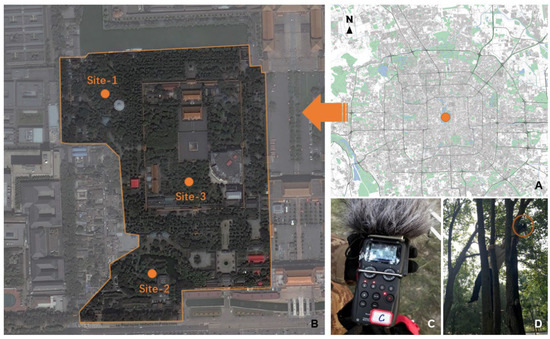
Figure 1.
Location of the urban forest (A); location of sites used for acoustic recording (B); an acoustic recorder (C) and its positioning in the urban forest (D) are also presented.
Our data were derived from audio recordings continuously obtained during four consecutive sunny, windless days, from 18 to 21 May 2019, provided by three recorders positioned in Zhongshan Park (Figure 1B). Recorders were placed and fixed horizontally at a height of 2 m on healthy growing trees (Figure 1C,D). Auto-recording led to a total of 17,280 min of raw recordings, which were subsequently processed using the AudioSegment function in PYTHON v.3.7.2 and sampled into 15-s clips every 15 min, resulting in a sub-dataset of 1152 15-s clips. A sampling protocol of 15 s was used as it provided a tradeoff between ensuring an effective acoustic survey and a manageable amount of data for processing when there is no standardized protocol [57].
Recordings were obtained using Zoom H5 acoustic sensors (Zoom Inc., Tokyo, Japan, System 2.40) with XYH-5 X/Y microphones. Zoom H5 is a commercial digital recording device that has good sound reliability and has been successfully used in other soundscape ecology research [27,58]. Parameters of sensors were set as follows: the sampling rate was 44,100 Hz, bit depth 16 bits, and recording channels two (stereo). Files were saved as non-compressed WAVE files.
Two trained technicians (Yu and Hanchen Huang) manually identified the acoustic events (AEs) in all audio clips for further use in evaluating the reliability and sensitivity of our approach. Over 95% of biological acoustic events (BEs) were from birds; thus, only bird sounds were identified to the species level (List of Bird Species see Table A1), while BEs that were not bird sounds were identified to the family level. For example, cricket sounds were labelled Gryllidae. Because we were unable to distinguish individual animals based on their sounds, technicians identified and counted the total number of BEs for a given species (or family) in each clip. Anthropogenic and geophysical sounds were also counted and classified into AEs. The results of this process were finally confirmed by Hanchen Huang. Richness (S), Shannon’s diversity (H’) and Simpson’s diversity (λ) indices were calculated for each spectrogram (i.e., per 15 s clip) to reflect the diversity of bird species as well as AE and BE types [12].
2.2. Methods
We developed an automated bird vocalization extraction approach based on OBIA, which followed a typical analysis workflow of bird vocalizations with three main steps [59]: preprocessing, automated extraction, and feature calculation. In line with this workflow, the processing details of each step of our approach are described in the following subsections. An overview of the approach is depicted in Figure 2.
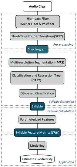
Figure 2.
Overall scheme of the proposed approach.
2.2.1. Pre-Processing
- Audio recordings denoising
The step prior to spectrogram analysis was denoising, and it was carried out to obtain clear vocalization patterns to improve extraction accuracy and minimize false positives [60]. We selected only noise reduction techniques that could perform batch and fast processing, to allow the proposed approach to be more generalizable and to reduce the effects of human operations.
Audio signals are characterized by the presence of higher energy in the low-frequency regions dominated by environmental noise. Therefore, we applied a high-pass filter with a cut-off frequency setting (800 Hz) below the lowest frequency at which bird songs are expected, with a 12 dB roll-off per octave [61,62,63,64]. This allowed for the elimination of current and environmental noise, mostly created by mechanical devices such as engines [65,66].
Since medium and high frequencies are the useful part for discriminating between different acoustic events [67], we applied a widely used signal enhancement method to our recordings, the Wiener filter [68,69,70] and postfilter, to minimize baseline and white noise and improve the quality of bird sound recordings. In field recordings, bird songs are transient but a considerable amount of background noise is nearly stationary. The Wiener filter eliminates this quasi-stationary noise, provided that it approximates a Gaussian distribution [22].
To verify the denoising effect, we randomly chose 80 clips from all datasets (including anthropogenic AEs) that were listened to before and after the denoising process to assess denoising efficacy.
- 2
- Short-time Fourier transformation (STFT)-Spectrogram
Bird vocalizations of songs or calls are complex, non-stationary signals with a great degree of variation in intensity, pitch, and syllable patterns [71]. One of the proven methods for joint time-frequency domain analysis of non-stationary sound signals is STFT [59]. The STFT spectrogram is a two-dimensional convolution of the signal and window function [72]: the X-axis represents time, the Y-axis represents frequency, and the amplitude of a particular frequency at a particular time is represented by its color in the image [73].
Our STFT spectrogram was calculated with a Hamming window of 1024 samples, no zero paddings, and a 75% overlap between successive windows. A peak amplitude of −25 dB was set to standardize the spectrograms [42].
2.2.2. Bird Vocalization Extraction
Generally, bird vocalizations are classified into songs (longer-term) and calls (shorter-term). In the present study, the separation between songs and calls was not considered because both types use syllables as fundamental units [74]. All vocalizations were segmented and classified at the syllable level. To facilitate understanding, a BE refers to either a song (call) in recordings or a syllable in spectrograms [10].
Bird syllable extraction is the key part of the proposed OBIA. All processing steps were conducted in one framework. Firstly, we adopted a multi-resolution segmentation algorithm to segment spectrograms into image objects. Then, we manually selected samples representing a pure spectrum of bird syllables to generate potential extraction features using a Classification and Regression Tree (CART). Finally, to extract bird syllables from background noise, we applied the rulesets established from identified potential features to all spectrograms.
- Segmentation
Segmentation creates new meaningful image objects according to their spectral properties (Figure 3), including subdividing and merging operations [75]. We applied the MRS algorithm embedded in eCognition Developer™ to generate image objects. This algorithm consecutively merges pixels or existing image objects into larger objects based on relative homogeneity within the merged object [53,54,76]. The process uses three key parameters in the process: scale, shape and compactness [77]. A coarse scale value allows for the forming of larger objects and more heterogeneity, involving more spectral values. Shape defines the influence of color (spectral value) and shapes on the formation of the segments, while compactness defines whether the boundary of the segments should be smoother or more compact [78]. In our segmentation, we employed the “trial and error” method of visual inspection to determine the optimal segmentation parameters [53], as bird syllables and their shapes on spectrograms are easily recognized by human eyes. After several attempts, we finally selected a scale of 40, 0.2 of shape, and 0.5 of compactness to produce segmented image objects.
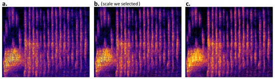
Figure 3.
Segmented image objects with three different scales but identical shape and compactness. (a) Scale 20 (1657 objects); (b) Scale 40 (458 objects); (c) Scale 60 (174 objects).
- 2
- Classification
Techniques from machine learning and computational intelligence have been used in bird vocalization analysis [79,80]. In the present study, CART [81] was applied to construct accurate and reliable predictive models for syllable extraction. CART does not require any special data preparation, only a good representation of the problem. Creating a CART model involves selecting input variables and split points on those variables until a suitable tree is trained. To operate CART, we randomly selected 288 syllable samples, one for each of the 288 audio clips, and divided them into training samples (70%, n = 202) and testing samples (30%, n = 86). Meanwhile, the ten most explanatory object features, including spectral, shape and textural characteristics (Table 1), were identified by calculating the feature variations in syllable samples and other objects, and were imported into CART as input variables. The representation of the CART model is a binary tree derived from recursive binary splitting (or greedy splitting). The binary tree allows for relatively straightforward obtainment of clear classification rules from the model diagram.

Table 1.
The summary of the 10 most explanatory object features used in CART.
The complexity of a decision tree is defined by the number of splits in each tree. Simpler trees are preferred, as they are easier to understand and less likely to overfit the data. Trees can be pruned to further improve performance. The fastest and simplest pruning method is to work through each leaf node in the tree and evaluate the effect of removing it using a hold-out test set. Leaf nodes are removed only if this results in a decrease in the overall cost function for the entire test set. Node removal is stopped when no further improvements can be made.
We introduced two indicators, relative cost (RC) and rate of change (ROC), to evaluate the performance of the CART model. The value of RC ranges from 0 to 1, with 0 indicating a perfect model with no error and 1 indicating random guessing. Similarly, the value of ROC ranges from 0 to 1, with higher values suggesting better performance. The resulting optimal decision tree consisted of three features: brightness, intensity, and grey level co-occurrence matrix (GLCM) homogeneity (Figure 4). It had an RC of 0.124 and a ROC of 0.979, indicating the reliability of the prediction model. The final step was to apply the ruleset generated from CART to classify all image objects.
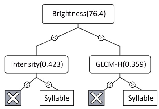
Figure 4.
The optimal decision tree resulting from CART. Instances with a split value greater than the threshold (in parentheses) were moved to the right.
2.2.3. Feature Representation of Extracted Syllables
The time-frequency pattern of syllables displayed via spectrograms is a useful representation of species information, which can also characterize bird vocalization patterns [82,83]. Based on the remote sensing framework, where syllables on spectrograms are comparable to landscape patches on maps, our approach could easily calculate and analyze morphological descriptors. Each extracted syllable was characterized by a sequence of feature vectors.
Considering their good performance with respect to feature analysis of syllables in previous studies, instantaneous frequency (IF) [59], and amplitude [84] were adopted in this work. Each parameter was further statistically analyzed to obtain more detailed descriptive values such as maximum (IF_MAX), minimum (IF_MI), mean, and central frequency. The mean instantaneous frequency (IF_MN) is the first moment of the spectrogram relative to the frequency, and it can be calculated using Equation (1):
where fi(t) is the mean instantaneous frequency at time t, and S (t, f) is the spectrogram at frequency f and time t.
In addition to the time-frequency characteristics, we also summarized the landscape metrics that were of practical meaning for syllable patches. Datasets were rasterized in R (https://www.r-project.org (accessed on 28 May 2021)) and imported into FRAGSTATS [85]. For each extracted syllable (patch level), we calculated area, shape index, border index, length, width (duration), etc., to obtain the fundamental spatial character and morphological understanding of each patch. Landscape-level metrics were also further summarized and nondimensionalized in each spectrogram, reflecting time-frequency patterns of acoustic activities, including: (1) NP, the number of syllable patches; (2) CA, the sum of the areas of all patches; (3) SHAPE_MN, mean value of the shape index of each patch; (4) TL, total bandwidth occupancy of all patches, calculated from a transformation of patch length; and (5) TW, total duration of all patches, calculated from a transformation of patch width. To facilitate reading, we abbreviated all these syllable feature metrics as SFMs (Table 2).
Table 2.
Summary of the main syllable feature metrics (SFMs).
2.3. Statistical Analysis
All statistical analyses were performed in R version 4.0.5 (R Core Team, Vienna, Austria, 2021).
Because the probability distribution of the raw data failed the Kolmogorov–Smirnov test for normality, transformations were performed using the bestNormalize package [86], which attempts a range of transformations and selects the best one based on the goodness-of-fit statistic to ensure transformations are consistent. It can also remove the effects of order-of-magnitude differences among variables.
2.3.1. Accuracy Assessment
Manual inspection of BEs from audio clips was used as a reference for accuracy assessment. To minimize errors, we marked each syllable patch with a serial number when calculating it to avoid missing or double-counting. We also recorded the time spent by the technician on each spectrogram. We used relative error (RE) as a measurement of accuracy, which is the ratio of the absolute value of the reference value [87]. Specifically, RE was calculated by dividing the number of syllables correctly identified through the automated approach by the total number of BEs identified through manual inspection as a reference.
2.3.2. Correlation Analysis
Correlation analysis (Spearman’s rho, p < 0.01) was performed between the number of extracted syllable patches and bioacoustic and acoustic events to further verify the reliability of the approach of automated extraction of bird vocalizations. Then, a second Spearman’s rho correlation test was performed for the relationships between SFMs and bird species S. Non-parametric correlation analysis was selected because not all data were normally distributed despite being transformed.
2.3.3. Modelling
To test the efficacy of SFMs as a biodiversity proxy, we used a random forest (RF) machine learning procedure (randomForest package) [88,89] to predict bird species biodiversity from SFMs calculated from matching recordings.
RF is a meta-estimator and one of the most accurate learning algorithms available. The RF algorithm aggregates many decision trees and combines the results of multiple predictions, while ensuring that the ensemble model makes fair use of all potentially predictive variables and prevents overfitting [90]. In addition, RF accommodates multivariate collinearity among predictors, which is convenient for calculating the nonlinear effects of variables [27]. We used a bootstrapping cross-validation method to select the model structure with the lowest median of mean squared error (MSE) and highest R2 between tested data and predicted values [12]. MSE was also used to measure the importance of each variable. A higher percentage increase in MSE indicated a greater ability to predict the model [91].
3. Results
3.1. Approach Reliability
With pre-processing denoising, we removed more than 85% (n = 77) of the anthropogenic acoustic events (for a denoising example see Figure 5A,B). The number of syllables identified from the spectrograms varied from 0 to 183 in each spectrogram according to the automatic extraction approach. The REs of the approach ranged from 11.52% to 0.00% across all spectrograms with an average of 6.45% (±4.78%), suggesting that the automated extraction process yielded high accuracy (93.55%) values (for an example of identified syllables see Figure 5).
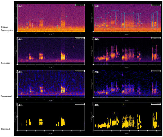
Figure 5.
Typical spectrograms of audio scenes during processing procedures. (A1,A2) is the original spectrogram. (B1,B2) shows the result of noise reduction: a cleaner recording (although possibly with some artifacts) that is ready to be used as input into segmentation algorithms. (C1,C2) shows the result of the segmentation procedure and (D1,D2) shows the classification results; the yellow patches are the extracted syllables.
A high correlation coefficient between the NP values and the number of bio-acoustic events and all acoustic events (r = 0.71, p < 0.01; r = 0.89, p < 0.01) was observed for the Spearman’s rho correlation matrix (Table 3). The CA (area), TL (duration) and TW (frequency) values of extracted syllables were also significantly correlated with bio-acoustic events and all acoustic events, albeit less strongly (Table 3).
Table 3.
Spearman’s rho correlation matrix (p < 0.01; n = 288).
These results indicate that this new, automated approach was much more efficient than manual inspection. For manual inspection, on average, it took approximately 27 s of effort to analyze 15-s acoustic data, which was approximately eight times longer than the time required for the automated approach (3.5 s refers to the time taken for the whole process shown in Figure 2, averaged by each 15 s-spectrogram). This is because analysts tend to replay recordings to confirm results [92], and the time spent on loading and annotating vocalizations must also be accounted for. Further, it is expected that the difference in efficiency would be more significant with increasing amounts of data, because spectrograms can be batch processed using our approach.
3.2. SFMs’ Correlation with Biodiversity
High correlation coefficients (r > 0.5) between SFMs and bird species richness were found, except for shape index and MIF (avg, min, and max) (Figure 6). Simpson’s and Shannon’s diversity indices were also correlated with SFMs, albeit less strongly. PN always had the highest correlation with the three diversity indices.
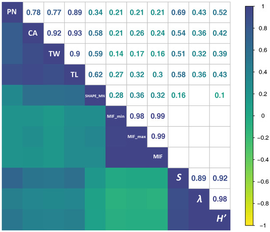
Figure 6.
Spearman’s correlation coefficient values shown for each relationship in the upper half of the matrix (only showing coefficient values that are statistically significant, p < 0.001). The diagonal shows the variables. Labels: NP = the number of syllable patches, CA = the sum of the areas of all patches in the given spectrogram, SHAPE_MN = the average shape index of patches across the entire spectrogram, TW = total duration of all patches in the given spectrogram (s), TL = total bandwidth occupancy of all patches in the given spectrogram (Hz), MIF = the mean instantaneous frequency (Hz), MIF_min = the minimum instantaneous frequency (Hz). MIF_min = the maximum instantaneous frequency (Hz). S = bird species richness, λ = Simpson’s Diversity Index, H’ = Shannon’s diversity index.
3.3. Prediction of Biodiversity
Random forest regression models confirmed that combinations of SFMs are good predictors of biodiversity (Table 4). Bird species richness was predicted well (R2 = 0.57) but the acoustic diversity of bird communities was less reliably predicted (Simpson’s and Shannon’s diversity indices had R2 of 0.38 and 0.41, respectively). These results suggest that SFMs have great potential for tracking acoustic communities, even in the presence of considerable anthrophony (human-induced noise) in an urban environment [29,93].
Table 4.
Mean squared error (MSE) and R2 of the top models of SFMs that predicted species richness, Shannon diversity, and Simpson diversity in acoustic recording samples.
We used all 14 SFMs as predictors (including soundscape and patch levels) in each RF regression model and investigated the relative contributions of each SFM. These metrics described soundscapes (syllable patches) from different perspectives and levels. Results demonstrated that SFMs effectively explained different pieces of information in acoustic recordings, likely because their unique mathematical properties reflect different dimensions of a soundscape. The number of syllable patches (PN) was the strongest single predictor in the best model found for richness (Figure 7a). In the best models predicting Simpson’s and Shannon’s diversity, the SFM with the highest importance was the total length of patches (20% and 23% of variance explained, respectively) (Figure 7b,c). It is noteworthy that PN, TL, and PI (Patch Intensity) were always the top three predictors for the three models (the sum of their contributions was 68%, 57%, and 65% in models a, b, and c respectively), suggesting that PN, TL and PI can be considered the most promising SFMs. All other indices exceeded the analytic threshold [63,94], suggesting that they all contributed little to predictive power.
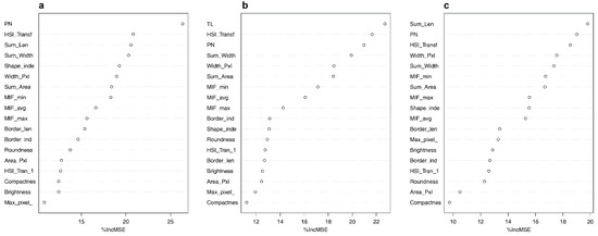
Figure 7.
Importance of covariates in random forest models, indicated by mean percent increase in mean squared error (MSE): the final models. (a) Richness of bird species, (b) Simpson diversity, and (c) Shannon diversity. Greater MSE indicates a larger loss of predictive accuracy when covariates are permuted and thus a larger influence in the model. Results are shown for acoustic index covariates, ordered by MSE. See Appendix A for a description of all SFMs.
4. Discussion
When analyzing biophony in urban environments, anthrophony could lead to potential false positives [95]. Low recognition accuracy is often attributed to noise [96], which affects the whole process unless removed initially. Hence, at present, most methods for analyzing biophony in urban environments are trained and tested on relatively low numbers of high-quality recordings that have been carefully selected [22]. This may lead to better results but will limit the generalization of their approach to real field recordings, especially in urban areas with complex acoustic environments. Therefore, in our study, we used only noise reduction, which meant that batch and fast processing could be performed.
According to Spearman’s rho correlations, NP was always more strongly correlated with AEs than with BEs, suggesting that SFMs were still somewhat influenced by human-generated noise, even after the denoising process. SFMs were hardly affected by constant-intensity noise (e.g., noise from aircraft or automobile traffic; for an example see Figure 5D: persistent noise was not extracted by the algorithm) [29,33]. In addition to pre-processing filtering, which eliminated most of the noise, CART models minimized the confounding effects of noise and syllables through training samples. The inherent properties of constant-intensity noise are different from those of bird vocalizations and are easily recognized by the model. For example, the brightness (Figure 4) of bird vocalizations was generally greater than 80, while the values for noise were 30–60. Nevertheless, some intermittent human noises, such as car horns and ringtones, might be extracted together with bird vocalizations using our approach. However, we believe that testing the approach in other habitats such as natural forests or biodiversity conservation areas will yield more encouraging results.
By treating spectrograms as images, previous studies have applied image processing techniques to extract bird vocalizations [10,59,60,83,96,97,98], such as widely used median clipping [41,99,100] and frame- or acoustic event-based morphological filtering [66]. There are plenty of toolboxes available to extract acoustic traits [22], such as central frequency, highest frequency, lowest frequency, initial frequency, and loudest frequency and so on [10,59], which are basically time–frequency characteristics only. To the best knowledge, all these studies aimed to identify or classify one or several bird species specifically. However, when focusing on the entire ecosystem, the species-level approach misses the forest for the trees [101]. Unlike the studies aiming at recognition of one or more species, ours attempted to take a global estimate of the acoustic output of the community. Our results indicated that SFMs are a promising complement to the existing indices working as biodiversity proxies when rapid assessments are required because SFMs were significantly correlated with diversity indices. SFMs allow for the effective interpretation of different pieces of bio-information in recordings, probably because their unique mathematical properties reflect different components of the soundscape, preserving more of the potentially eco-relevant information.
Using the proposed approach, we could collect a series of data including acoustic traits on the time–frequency scale (Figure 8), such as duration and mean, maximum, and minimum frequency of acoustic events, and morphological characteristics of acoustic events (Figure 9), such as the size and shape characteristics for each syllable patch. Such features (i.e., SFMs) may contribute to a more nuanced understanding of the acoustic environment of the study area from multiple perspectives. In Figure 8, the frequency patterns of syllable patches are shown across frequency intervals. The soundscape was dominated by mid-frequency sounds (3–5 kHz); syllable patches were over 50%. Mid-frequency sounds are generally attributed to biophony, especially bird species ranging from larger birds such as the Eurasian magpie (Pica pica) to smaller species such as the Oriental reed warbler (Acrocephalus orientalis). At the other end of the frequency spectrum, the number of patches within individual high-frequency intervals was quite low (biophony patches in the highest four frequency intervals accounted for 1.5%) and were mainly within 20–22 kHz, which may be attributed to some night-flying moths of the family Noctuidae or to mating calls from grasshoppers. In Figure 9, the average shape index (SHAPE) over 24 h was shown to rise rapidly at dawn chorus to reach the peak of the day, falling rapidly and remaining steady until dusk, when the chorus rose rapidly again, and then fluctuated and fell until the morning. The daily pattern of SHAPE is consistent with previous studies of other acoustic indices [27,31,102,103], thus reflecting a daily activity pattern and highlighting distinct dawn and dusk bird choruses. However, compared to other indices that only focus on sound intensity, SHAPE provides a new perspective on patterns of complexity of bird songs: songs of the dawn and dusk choruses tended to be more complex and elaborate than daytime songs. This is mainly related to defending territory and/or attracting a mate [104].
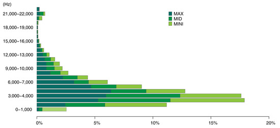
Figure 8.
Number of maximum, medium, and minimum frequencies for each syllable patch across 23 1-kHz intervals.
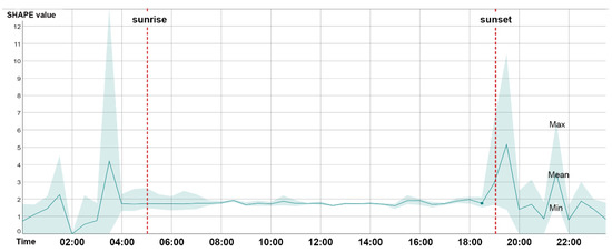
Figure 9.
Shape index variation for 24 h. Upper bound is the maximum. Lower bound is the minimum.
Borrowing a framework from landscape ecology, many types SFMs can effectively be used to interpret different aspects of acoustic information and different components of the soundscape, which is presumably attributed to the mathematical properties of SFMs and to the introduction of a spatial concept. SFMs calculated in this study, such as area, compactness, roundness, and shape index of the patches, could be easily generated in eCognition developer. In addition, many existing open-source platforms (e.g., package landscapemetrics in R) or software have integrated huge workflows, which can provide similar functions (e.g., QGIS). Measurement of biophony from multiple dimensions has been considered useful for detecting variations in the behavior and composition of acoustic communities and, as a result, to better monitor their dynamics and interactions with habitats [29]. These results support the possibility that PAM could potentially offer a more comprehensive picture of biodiversity than traditional inspection [63].
Under the high pressure of a surplus of data, and facing the lack of technology, funding and standardized protocols [11], most passive monitoring now lasts one to three years at most [105], while ecosystem conservation and ecological change detection usually require at least ten years. In particular, there is usually a lag period when measuring the benefits of planted forests, as individual trees need to grow and stands need to mature to form a stable structure [4]. Short-term monitoring may lead to a reduction in the quality and reliability of data [106]. This emphasizes the significance of utilizing and applying PAM within the framework of a monitoring strategy, with defined objectives, effective indicators, and standardized protocols [20].
There is developing acknowledgment from governments and related sectors that urban greenery is not monitored adequately to satisfy its crucial roles in biodiversity provisioning and ecosystem support [33,107]. A rich and diverse biophony usually indicates a stable and healthy ecosystem [26]. With its government-led design, planning, and implementation, the in-depth greening project in Beijing has indeed enhanced green space in the plain area, if only considering the total increased amounts of trees and connected urban forest and park patches [108]. However, the large-scale transition between cropland and forest generated by the afforestation process has the potential to lead to original wildlife habitat loss. By long-term monitoring of biodiversity patterns and processes, we can better assess the positive and negative impacts of afforestation projects.
According to our preliminary results, the proposed approach (with high computational efficiency and accuracy) may benefit further research on the rapid assessment and prediction of biodiversity in urban forests, providing an indirect but immediate measurement of bird activity dynamics across enhanced spatio-temporal scales. This would facilitate the application of PAM and the formulation of a standardized sampling protocol. Furthermore, a robust automated approach could support PAM as part of citizen science research. This would benefit developing countries that lack financial budgets, experts, and capacity for massive data processing. Globally, only 5% of PAM studies are conducted in regions of Asia, western Oceania, northern Africa, and southern South America, where some countries still have no record of using PAM [20]. As our approach does not require a priori data, it facilitates the implementation of long-term ecosystem monitoring in developing countries where baseline data are not available.
5. Conclusions
In 2019, the Intergovernmental Science-Policy Platform on Biodiversity and Ecosystem Services (IPBES) warned that the unprecedented deterioration of natural resources was deracinating millions of species and reducing human well-being worldwide. However, global biodiversity loss has not attracted as much public attention as global climate change. To evaluate the diversity of coexisting birds in urban forests and ultimately facilitate the assessment of afforestation benefits in urbanized Beijing, we developed an automated approach to extract and quantify bird vocalizations from spectrograms, integrating the well-established technology of object-based image analysis. The approach could achieve recognition accuracy (93.55%) of acoustic events at much higher efficiency (eight times faster) than traditional inspection methods. In addition, it also provided multiple aspects of acoustic traits, such as quantity, song length, frequency bandwidth, and shape information, which can be used to predict bird biodiversity. In our case, 57% of the variance in bird species richness could be explained by the acoustic and morphological features selected. The proposed soundscape evaluation method sheds light on long-term biodiversity monitoring and conservation during the upcoming global biodiversity crisis.
Author Contributions
Conceptualization, Y.Z., J.Y. and C.W.; data curation, Y.Z. and Z.B.; formal analysis, Y.Z. and J.Y.; funding acquisition, C.W.; investigation, Y.Z. and Z.B.; methodology, Y.Z., J.Y. and J.J.; project administration, C.W.; resources, Z.S., L.Y. and C.W.; software, Y.Z. and J.Y.; validation, Y.Z., J.Y., J.J., Z.S., L.Y. and C.W.; visualization, Y.Z.; writing—original draft, Y.Z.; writing—review and editing, J.Y., J.J. and C.W. All authors have read and agreed to the published version of the manuscript.
Funding
This research was funded by the National Non-Profit Research Institutions of the Chinese Academy of Forestry (CAFYBB2020ZB008).
Institutional Review Board Statement
Not applicable.
Informed Consent Statement
Not applicable.
Data Availability Statement
Not applicable.
Acknowledgments
We thank Hanchen Huang for bird species identification, Junyou Zhang for writing advice, and Shi Xu, Qi Bian for field investigation.
Conflicts of Interest
The authors declare no conflict of interest.
Appendix A
Table A1.
List of Bird Species. A total of 30,758 vocalizations pertaining to 33 species were counted during recording sessions, as shown in the table below.
Table A1.
List of Bird Species. A total of 30,758 vocalizations pertaining to 33 species were counted during recording sessions, as shown in the table below.
| No. | Common Name | Binomial Name | Number of Syllable Patches | % | Predominant Frequency Intervals |
|---|---|---|---|---|---|
| 1 | Common Blackbird | Turdus merula | 227 | 23.67049 | / |
| 2 | Eurasian tree sparrow | Passer montanus | 158 | 16.4755 | 2.3–5 kHz or |
| 3 | Azure-winged magpie | Cyanopica cyanus | 120 | 12.51303 | 2–10 kHz |
| 4 | Large-billed crow | Corvus macrorhynchos | 116 | 12.09593 | 1–2 kHz |
| 5 | Spotted dove | Spilopelia chinensis | 109 | 11.36601 | 1–2 kHz |
| 6 | Light-vented bulbul | Pycnonotus sinensis | 55 | 5.735141 | 1.5–4 kHz |
| 7 | Eurasian magpie | Pica pica | 46 | 4.796663 | 0–4 kHz |
| 8 | Common swift | Apus apus | 42 | 4.379562 | 20–16,000 Hz |
| 9 | Yellow-browed warbler | Phylloscopus inornatus | 17 | 1.77268 | 4–8 kHz |
| 10 | Arctic warbler | Phylloscopus borealis | 12 | 1.251303 | / |
| 11 | Crested myna | Acridotheres cristatellus | 7 | 0.729927 | / |
| 12 | Two-barred warbler | Phylloscopus plumbeitarsus | 7 | 0.729927 | / |
| 13 | Dusky warbler | Phylloscopus fuscatus | 6 | 0.625652 | / |
| 14 | Marsh tit | Poecile palustris | 5 | 0.521376 | 6–10 kHz |
| 15 | Grey starling | Spodiopsar cineraceus | 4 | 0.417101 | above 4 kHz |
| 16 | Great spotted woodpecker | Dendrocopos major | 4 | 0.417101 | 0–2.6 kHz |
| 17 | Chinese grosbeak | Eophona migratoria | 4 | 0.417101 | / |
| 18 | Barn swallow | Hirundo rustica | 3 | 0.312826 | / |
| 19 | Chicken | Gallus gallus domesticus | 2 | 0.208551 | 5–10 kHz |
| 20 | Grey-capped greenfinch | Chloris sinica | 2 | 0.208551 | 3–5.5 kHz |
| 21 | Yellow-rumped Flycatcher | Ficedula zanthopygia | 1 | 0.104275 | / |
| 22 | Oriental reed warbler | Acrocephalus orientalis | 1 | 0.104275 | / |
| 23 | Yellow-throated Bunting | Emberiza elegans | 1 | 0.104275 | / |
| 24 | Red-breasted Flycatcher | Ficedula parva | 1 | 0.104275 | / |
| 25 | Carrion crow | Corvus corone | 1 | 0.104275 | 0–8 kHz |
| 26 | Dusky thrush | Turdus eunomus | 1 | 0.104275 | / |
| 27 | Black-browed Reed Warbler | Acrocephalus bistrigiceps | 1 | 0.104275 | / |
| 28 | Grey-capped pygmy woodpecker | Dendrocopos canicapillus | 1 | 0.104275 | 4.5–5 kHz |
| 29 | Naumann’s Thrush | Turdus naumanni | 1 | 0.104275 | / |
| 30 | U1 | / | 1 | 0.104275 | / |
| 31 | U2 | / | 1 | 0.104275 | / |
| 32 | U3 | / | 1 | 0.104275 | / |
| 33 | U4 | / | 1 | 0.104275 | / |
Note: Unidentified species marked as U1-Un.
Table A2.
List of other SFMs.
Table A2.
List of other SFMs.
| No. | Metric | Description |
|---|---|---|
| 1 | Border_len(Border Length) | The sum of the edges of the patch. |
| 2 | Width_Pxl (Width) | The number of pixels occupied by the length of the patch. |
| 3 | HSI_Transf | HSI transformation feature of patch hue. |
| 4 | HSI_Tran_1 | HSI transformation feature of patch intensity. |
| 5 | Compactnes | The Compactness feature describes how compact a patch is. It is similar to Border Index but is based on area. However, the more compact a patch is, the smaller its border appears. The compactness of a patch is the product of the length and the width, divided by the number of pixels. |
| 6 | Roundness | The Roundness feature describes how similar a patch is to an ellipse. It is calculated by the difference between the enclosing ellipse and the enclosed ellipse. The radius of the largest enclosed ellipse is subtracted from the radius of the smallest enclosing ellipse. |
| 7 | Area_Pxl (Area of the patch) | The number of pixels forming a patch. If unit information is available, the number of pixels can be converted into a measurement. In scenes that provide no unit information, the area of a single pixel is 1 and the patch area is simply the number of pixels that form it. If the image data provides unit information, the area can be multiplied using the appropriate factor. |
| 8 | Border_ind (Border index) | The Border Index feature describes how jagged a patch is; the more jagged, the higher its border index. This feature is similar to the Shape Index feature, but the Border Index feature uses a rectangular approximation instead of a square. The smallest rectangle enclosing the patch is created and the border index is calculated as the ratio between the border lengths of the patch and the smallest enclosing rectangle. |
References
- Zhongming, Z.; Linong, L.; Wangqiang, Z.; Wei, L. The Global Biodiversity Outlook 5 (GBO-5); Secretariat of the Convention on Biological Diversity: Montreal, QC, Canada, 2020. [Google Scholar]
- World Health Organization. WHO-Convened Global Study of Origins of SARS-CoV-2: China Part; WHO: Geneva, Switzerland, 2021. [Google Scholar]
- Platto, S.; Zhou, J.; Wang, Y.; Wang, H.; Carafoli, E. Biodiversity loss and COVID-19 pandemic: The role of bats in the origin and the spreading of the disease. Biochem. Biophys. Res. Commun. 2021, 538, 2. [Google Scholar] [CrossRef]
- Pei, N.; Wang, C.; Jin, J.; Jia, B.; Chen, B.; Qie, G.; Qiu, E.; Gu, L.; Sun, R.; Li, J.; et al. Long-term afforestation efforts increase bird species diversity in Beijing, China. Urban For. Urban Green. 2018, 29, 88. [Google Scholar] [CrossRef]
- Turner, A.; Fischer, M.; Tzanopoulos, J. Sound-mapping a coniferous forest-Perspectives for biodiversity monitoring and noise mitigation. PLoS ONE 2018, 13, e0189843. [Google Scholar] [CrossRef] [Green Version]
- Sueur, J.; Gasc, A.; Grandcolas, P.; Pavoine, S. Global estimation of animal diversity using automatic acoustic sensors. In Sensors for Ecology; CNRS: Paris, France, 2012; Volume 99. [Google Scholar]
- Sueur, J.; Farina, A. Ecoacoustics: The Ecological Investigation and Interpretation of Environmental Sound. Biosemiotics 2015, 8, 493. [Google Scholar] [CrossRef]
- Blumstein, D.T.; Mennill, D.J.; Clemins, P.; Girod, L.; Yao, K.; Patricelli, G.; Deppe, J.L.; Krakauer, A.H.; Clark, C.; Cortopassi, K.A.; et al. Acoustic mon-itoring in terrestrial environments using microphone arrays: Applications, technological considerations and prospectus. J. Appl. Ecol. 2011, 48, 758. [Google Scholar] [CrossRef]
- Krause, B.; Farina, A. Using ecoacoustic methods to survey the impacts of climate change on biodiversity. Biol. Conserv. 2016, 195, 245. [Google Scholar] [CrossRef]
- Zhao, Z.; Zhang, S.; Xu, Z.; Bellisario, K.; Dai, N.; Omrani, H.; Pijanowski, B.C. Automated bird acoustic event detection and robust species classification. Ecol. Inform. 2017, 39, 99. [Google Scholar] [CrossRef]
- Stephenson, P.J. Technological advances in biodiversity monitoring: Applicability, opportunities and challenges. Curr. Opin. Environ. Sustain. 2020, 45, 36. [Google Scholar] [CrossRef]
- Buxton, R.T.; McKenna, M.F.; Clapp, M.; Meyer, E.; Stabenau, E.; Angeloni, L.M.; Crooks, K.; Wittemyer, G. Efficacy of extracting indices from large-scale acoustic recordings to monitor biodiversity. Conserv. Biol. 2018, 32, 1174. [Google Scholar] [CrossRef]
- Halpin, P.N.; Read, A.J.; Best, B.D.; Hyrenbach, K.D.; Fujioka, E.; Coyne, M.S.; Crowder, L.B.; Freeman, S.; Spoerri, C. OBIS-SEAMAP: Developing a biogeographic research data commons for the ecological studies of marine mammals, seabirds, and sea turtles. Mar. Ecol. Prog. Ser. 2006, 316, 239. [Google Scholar] [CrossRef]
- Gross, M. Eavesdropping on ecosystems. Curr. Biol. 2020, 30, R237–R240. [Google Scholar] [CrossRef]
- Rajan, S.C.; Athira, K.; Jaishanker, R.; Sooraj, N.P.; Sarojkumar, V. Rapid assessment of biodiversity using acoustic indices. Biodivers. Conserv. 2019, 28, 2371. [Google Scholar] [CrossRef]
- Llusia, D.; Márquez, R.; Beltrán, J.F.; Benítez, M.; do Amaral, J.P. Calling behaviour under climate change: Geographical and seasonal variation of calling temperatures in ectotherms. Glob. Chang. Biol. 2013, 19, 2655. [Google Scholar] [CrossRef] [PubMed]
- Hart, P.J.; Sebastián-González, E.; Tanimoto, A.; Thompson, A.; Speetjens, T.; Hopkins, M.; Atencio-Picado, M. Birdsong characteristics are related to fragment size in a neotropical forest. Anim. Behav. 2018, 137, 45. [Google Scholar] [CrossRef]
- Bueno-Enciso, J.; Ferrer, E.S.; Barrientos, R.; Sanz, J.J. Habitat structure influences the song characteris-tics within a population of Great Tits Parus major. Bird Study 2016, 63, 359. [Google Scholar] [CrossRef]
- Browning, E.; Gibb, R.; Glover-Kapfer, P.; Jones, K.E. Passive Acoustic Monitoring in Ecology and Conservation. 2017. Available online: https://www.wwf.org.uk/sites/default/files/2019-04/Acousticmonitoring-WWF-guidelines.pdf (accessed on 7 April 2021).
- Sugai, L.S.M.; Silva, T.S.F.; Ribeiro, J.W.; Llusia, D. Terrestrial Passive Acoustic Monitoring: Review and Perspectives. BioScience 2019, 69, 15. [Google Scholar] [CrossRef]
- Righini, R.; Pavan, G. A soundscape assessment of the Sasso Fratino Integral Nature Reserve in the Central Apennines, Italy. Biodiversity 2020, 21, 4. [Google Scholar] [CrossRef]
- Priyadarshani, N.; Marsland, S.; Castro, I. Automated birdsong recognition in complex acoustic environments: A review. J. Avian Biol. 2018, 49, jav-01447. [Google Scholar] [CrossRef] [Green Version]
- Farina, A. Soundscape Ecology: Principles, Patterns, Methods and Applications; Springer: Berlin/Heidelberg, Germany, 2013. [Google Scholar]
- Eldridge, A.; Casey, M.; Moscoso, P.; Peck, M. A new method for ecoacoustics? Toward the extraction and evaluation of ecologically-meaningful soundscape components using sparse coding methods. PeerJ 2016, 4, e2108. [Google Scholar] [CrossRef] [Green Version]
- Lellouch, L.; Pavoine, S.; Jiguet, F.; Glotin, H.; Sueur, J. Monitoring temporal change of bird communities with dissimilarity acoustic indices. Methods Ecol. Evol. 2014, 5, 495. [Google Scholar] [CrossRef] [Green Version]
- Pijanowski, B.C.; Villanueva-Rivera, L.J.; Dumyahn, S.L.; Farina, A.; Krause, B.L.; Napoletano, B.M.; Gage, S.H.; Pieretti, N. Soundscape Ecology: The Science of Sound in the Landscape. BioScience 2011, 61, 203. [Google Scholar] [CrossRef] [Green Version]
- Hao, Z.; Wang, C.; Sun, Z.; van den Bosch, C.K.; Zhao, D.; Sun, B.; Xu, X.; Bian, Q.; Bai, Z.; Wei, K.; et al. Soundscape mapping for spa-tial-temporal estimate on bird activities in urban forests. Urban For. Urban Green. 2021, 57, 126822. [Google Scholar] [CrossRef]
- Project, W.S.; Truax, B. The World Soundscape Project’s Handbook for Acoustic Ecology; Arc Publications: Todmorden, UK, 1978. [Google Scholar]
- Pieretti, N.; Farina, A.; Morri, D. A new methodology to infer the singing activity of an avian community: The Acoustic Complexity Index (ACI). Ecol. Indic. 2011, 11, 868. [Google Scholar] [CrossRef]
- Boelman, N.T.; Asner, G.P.; Hart, P.J.; Martin, R.E. Multi-trophic invasion resistance in Hawaii: Bioacoustics, field surveys, and airborne remote sensing. Ecol. Appl. 2007, 17, 2137. [Google Scholar] [CrossRef]
- Fuller, S.; Axel, A.C.; Tucker, D.; Gage, S.H. Connecting soundscape to landscape: Which acoustic index best describes landscape configuration? Ecol. Indic. 2015, 58, 207. [Google Scholar] [CrossRef] [Green Version]
- Mammides, C.; Goodale, E.; Dayananda, S.K.; Kang, L.; Chen, J. Do acoustic indices correlate with bird diversity? Insights from two biodiverse regions in Yunnan Province, south China. Ecol. Indic. 2017, 82, 470. [Google Scholar] [CrossRef]
- Fairbrass, A.J.; Rennert, P.; Williams, C.; Titheridge, H.; Jones, K.E. Biases of acoustic indices measuring biodiversity in urban areas. Ecol. Indic. 2017, 83, 169. [Google Scholar] [CrossRef]
- Ross, S.R.-J.; Friedman, N.R.; Yoshimura, M.; Yoshida, T.; Donohue, I.; Economo, E.P. Utility of acoustic indices for ecological monitoring in complex sonic environments. Ecol. Indic. 2021, 121, 107114. [Google Scholar] [CrossRef]
- Sueur, J.; Pavoine, S.; Hamerlynck, O.; Duvail, S. Rapid acoustic survey for biodiversity appraisal. PLoS ONE 2008, 3, e4065. [Google Scholar] [CrossRef] [Green Version]
- Kasten, E.P.; Gage, S.H.; Fox, J.; Joo, W. The remote environmental assessment laboratory’s acoustic library: An archive for studying soundscape ecology. Ecol. Inform. 2012, 12, 50. [Google Scholar] [CrossRef]
- Gibb, R.; Browning, E.; Glover-Kapfer, P.; Jones, K.E. Emerging opportunities and challenges for passive acoustics in ecological assessment and monitoring. Methods Ecol. Evol. 2019, 10, 169. [Google Scholar] [CrossRef] [Green Version]
- Merchant, N.D.; Fristrup, K.M.; Johnson, M.P.; Tyack, P.L.; Witt, M.J.; Blondel, P.; Parks, S.E. Measuring acoustic habitats. Methods Ecol. Evol. 2015, 6, 257. [Google Scholar] [CrossRef] [PubMed] [Green Version]
- Swiston, K.A.; Mennill, D.J. Comparison of manual and automated methods for identifying target sounds in audio recordings of Pileated, Pale-billed, and putative Ivory-billed woodpeckers. J. Field Ornithol. 2009, 80, 42. [Google Scholar] [CrossRef]
- Goyette, J.L.; Howe, R.W.; Wolf, A.T.; Robinson, W.D. Detecting tropical nocturnal birds using auto-mated audio recordings. J. Field Ornithol. 2011, 82, 279. [Google Scholar] [CrossRef]
- Potamitis, I. Automatic classification of a taxon-rich community recorded in the wild. PLoS ONE 2014, 9, e96936. [Google Scholar]
- Ulloa, J.S.; Gasc, A.; Gaucher, P.; Aubin, T.; Réjou-Méchain, M.; Sueur, J. Screening large audio datasets to determine the time and space distribution of Screaming Piha birds in a tropical forest. Ecol. Inform. 2016, 31, 91. [Google Scholar] [CrossRef]
- Blaschke, T. Object based image analysis for remote sensing. ISPRS J. Photogramm. Remote Sens. 2010, 65, 2. [Google Scholar] [CrossRef] [Green Version]
- Blaschke, T. (Ed.) Object Based Image Analysis: A new paradigm in remote sensing? In Proceedings of the American Society for Photogrammetry and Remote Sensing Annual Conferenc, Baltimore, MD, USA, 26–28 March 2013. [Google Scholar]
- Benz, U.C.; Hofmann, P.; Willhauck, G.; Lingenfelder, I.; Heynen, M. Multi-resolution, object-oriented fuzzy analysis of remote sensing data for GIS-ready information. ISPRS J. Photogramm. Remote Sens. 2004, 58, 239. [Google Scholar] [CrossRef]
- Johansen, K.; Arroyo, L.A.; Phinn, S.; Witte, C. Comparison of geo-object based and pixel-based change detection of riparian environments using high spatial resolution multi-spectral imagery. Photogramm. Eng. Remote Sens. 2010, 76, 123. [Google Scholar] [CrossRef]
- Burivalova, Z.; Game, E.T.; Butler, R.A. The sound of a tropical forest. Science 2019, 363, 28. [Google Scholar] [CrossRef]
- Hay, G.J.; Castilla, G. Object-based image analysis: Strengths, weaknesses, opportunities and threats (SWOT). In Proceedings of the 1st International Conference on Object-based Image Analysis (OBIA), Salzburg, Austria, 4–5 July 2006; pp. 4–5. [Google Scholar]
- Jafari, N.H.; Li, X.; Chen, Q.; Le, C.-Y.; Betzer, L.P.; Liang, Y. Real-time water level monitoring using live cameras and computer vision techniques. Comput. Geosci. 2021, 147, 104642. [Google Scholar] [CrossRef]
- Schwier, M. Object-based Image Analysis for Detection and Segmentation Tasks in Biomedical Imaging. Ph.D. Thesis, Information Resource Center der Jacobs University Bremen, Bremen, Germany.
- Kerle, N.; Gerke, M.; Lefèvre, S. GEOBIA 2016: Advances in Object-Based Image Analysis—Linking with Computer Vision and Machine Learning; Multidisciplinary Digital Publishing Institute: Basel, Switzerland, 2019. [Google Scholar]
- Yan, J.; Lin, L.; Zhou, W.; Han, L.; Ma, K. Quantifying the characteristics of particulate matters captured by urban plants using an automatic approach. J. Environ. Sci. 2016, 39, 259. [Google Scholar] [CrossRef] [PubMed]
- Yan, J.; Lin, L.; Zhou, W.; Ma, K.; Pickett, S.T.A. A novel approach for quantifying particulate matter dis-tribution on leaf surface by combining SEM and object-based image analysis. Remote Sens. Environ. 2016, 173, 156. [Google Scholar] [CrossRef]
- Lin, L.; Yan, J.; Ma, K.; Zhou, W.; Chen, G.; Tang, R.; Zhang, Y. Characterization of particulate matter de-posited on urban tree foliage: A landscape analysis approach. Atmos. Environ. 2017, 171, 59. [Google Scholar] [CrossRef]
- Artiola, J.F.; Brusseau, M.L.; Pepper, I.L. Environmental Monitoring and Characterization; Academic Press: Cambridge, MA, USA, 2004. [Google Scholar]
- Xie, S.; Lu, F.; Cao, L.; Zhou, W.; Ouyang, Z. Multi-scale factors influencing the characteristics of avian communities in urban parks across Beijing during the breeding season. Sci. Rep. 2016, 6, 29350. [Google Scholar] [CrossRef] [PubMed]
- Farina, A.; Righini, R.; Fuller, S.; Li, P.; Pavan, G. Acoustic complexity indices reveal the acoustic commu-nities of the old-growth Mediterranean forest of Sasso Fratino Integral Natural Reserve (Central Italy). Ecol. Indic. 2021, 120, 106927. [Google Scholar] [CrossRef]
- Zitong, B.; Yilin, Z.; Cheng, W.; Zhenkai, S. The public’s Perception of Anthrophony Soundscape in Beijing’s Urban Parks. J. Chin. Urban For. 2021, 19, 16, In Chinese. [Google Scholar] [CrossRef]
- Pahuja, R.; Kumar, A. Sound-spectrogram based automatic bird species recognition using MLP classifier. Appl. Acoust. 2021, 180, 108077. [Google Scholar] [CrossRef]
- Aide, T.M.; Corrada-Bravo, C.; Campos-Cerqueira, M.; Milan, C.; Vega, G.; Alvarez, R. Real-time bioacous-tics monitoring and automated species identification. PeerJ 2013, 1, e103. [Google Scholar] [CrossRef] [Green Version]
- Linke, S.; Deretic, J.-A. Ecoacoustics can detect ecosystem responses to environmental water allocations. Freshw. Biol. 2020, 65, 133. [Google Scholar] [CrossRef] [Green Version]
- Gasc, A.; Francomano, D.; Dunning, J.B.; Pijanowski, B.C. Future directions for soundscape ecology: The importance of ornithological contributions. Auk 2017, 134, 215. [Google Scholar] [CrossRef] [Green Version]
- Eldridge, A.; Guyot, P.; Moscoso, P.; Johnston, A.; Eyre-Walker, Y.; Peck, M. Sounding out ecoacoustic met-rics: Avian species richness is predicted by acoustic indices in temperate but not tropical habitats. Ecol. Indic. 2018, 95, 939. [Google Scholar] [CrossRef] [Green Version]
- Dufour, O.; Artieres, T.; Glotin, H.; Giraudet, P. Soundscape Semiotics—Localization and Categorization; InTech: London, UK, 2013; Volume 89. [Google Scholar]
- Karaconstantis, C.; Desjonquères, C.; Gifford, T.; Linke, S. Spatio-temporal heterogeneity in river sounds: Disentangling micro-and macro-variation in a chain of waterholes. Freshw. Biol. 2020, 65, 96. [Google Scholar] [CrossRef]
- De Oliveira, A.G.; Ventura, T.M.; Ganchev, T.D.; de Figueiredo, J.M.; Jahn, O.; Marques, M.I.; Schuchmann, K.-L. Bird acoustic activity detection based on morphological filtering of the spectrogram. Appl. Acoust. 2015, 98, 34. [Google Scholar] [CrossRef]
- Ludeña-Choez, J.; Gallardo-Antolín, A. Feature extraction based on the high-pass filtering of audio signals for Acoustic Event Classification. Comput. Speech Lang. 2015, 30, 32. [Google Scholar] [CrossRef] [Green Version]
- Albornoz, E.M.; Vignolo, L.D.; Sarquis, J.A.; Leon, E. Automatic classification of Furnariidae species from the Paranaense Littoral region using speech-related features and machine learning. Ecol. Inform. 2017, 38, 39. [Google Scholar] [CrossRef]
- Bhargava, S. Vocal Source Separation Using Spectrograms and Spikes, Applied to Speech and Birdsong; ETH Zurich: Zurich, Switzerland, 2017. [Google Scholar]
- Plapous, C.; Marro, C.; Scalart, P. Improved signal-to-noise ratio estimation for speech enhancement. IEEE Trans. Audio Speech Lang. Process. 2006, 14, 2098. [Google Scholar] [CrossRef] [Green Version]
- Podos, J.; Warren, P.S. The evolution of geographic variation in birdsong. Adv. Study Behav. 2007, 37, 403. [Google Scholar]
- Lu, W.; Zhang, Q. Deconvolutive Short-Time Fourier Transform Spectrogram. IEEE Signal Process. Lett. 2009, 16, 576. [Google Scholar]
- Mehta, J.; Gandhi, D.; Thakur, G.; Kanani, P. Music Genre Classification using Transfer Learning on log-based MEL Spectrogram. In Proceedings of the 5th International Conference on Computing Methodolo-Gies and Communication (ICCMC), Erode, India, 8–10 April 2021; p. 1101. [Google Scholar]
- Ludena-Choez, J.; Quispe-Soncco, R.; Gallardo-Antolin, A. Bird sound spectrogram decomposition through Non-Negative Matrix Factorization for the acoustic classification of bird species. PLoS ONE 2017, 12, e0179403. [Google Scholar] [CrossRef]
- Garcia-Lamont, F.; Cervantes, J.; López, A.; Rodriguez, L. Segmentation of images by color features: A survey. Neurocomputing 2018, 292, 1. [Google Scholar] [CrossRef]
- Chen, Y.; Chen, Q.; Jing, C. Multi-resolution segmentation parameters optimization and evaluation for VHR remote sensing image based on mean NSQI and discrepancy measure. J. Spat. Sci. 2021, 66, 253. [Google Scholar] [CrossRef]
- Zheng, L.; Huang, W. Parameter Optimization in Multi-scale Segmentation of High Resolution Remotely Sensed Image and Its Application in Object-oriented Classification. J. Subtrop. Resour. Environ. 2015, 10, 77. [Google Scholar]
- Mesner, N.; Ostir, K. Investigating the impact of spatial and spectral resolution of satellite images on segmentation quality. J. Appl. Remote Sens. 2014, 8, 83696. [Google Scholar] [CrossRef]
- Ptacek, L.; Machlica, L.; Linhart, P.; Jaska, P.; Muller, L. Automatic recognition of bird individuals on an open set using as-is recordings. Bioacoustics 2016, 25, 55. [Google Scholar] [CrossRef]
- Yip, D.A.; Mahon, C.L.; MacPhail, A.G.; Bayne, E.M. Automated classification of avian vocal activity using acoustic indices in regional and heterogeneous datasets. Methods Ecol. Evol. 2021, 12, 707. [Google Scholar] [CrossRef]
- Breiman, L.; Friedman, J.H.; Olshen, R.A.; Stone, C.J. Classification and Regression Trees; Routledge: Oxfordshire, UK, 2017. [Google Scholar]
- Stowell, D.; Plumbley, M.D. Automatic large-scale classification of bird sounds is strongly improved by unsupervised feature learning. PeerJ 2014, 2, e488. [Google Scholar] [CrossRef] [Green Version]
- Zottesso, R.H.D.; Costa, Y.M.G.; Bertolini, D.; Oliveira, L.E.S. Bird species identification using spectro-gram and dissimilarity approach. Ecol. Inform. 2018, 48, 187. [Google Scholar] [CrossRef]
- Bai, J.; Chen, C.; Chen, J. (Eds.) Xception Based Method for Bird Sound Recognition of BirdCLEF; CLEF: Thessaloniki, Greece, 2020. [Google Scholar]
- McGarigal, K.; Cushman, S.A.; Ene, E. FRAGSTATS v4: Spatial Pattern Analysis Program for Categorical and Continuous Maps. Computer Software Program Produced by the Authors at the University of Massachusetts, Amherst. 2012. Available online: http://www.umass.edu/landeco/research/fragstats/fragstats.html (accessed on 25 June 2021).
- Peterson, R.A.; Peterson, M.R.A. Package ‘bestNormalize’. 2020. Available online: https://mran.microsoft.com/snapshot/2020-04-22/web/packages/bestNormalize/bestNormalize.pdf (accessed on 5 April 2021).
- Van Loan, C.F.; Golub, G. Matrix Computations (Johns Hopkins Studies in Mathematical Sciences); Johns Hopkins University Press: Baltimore, MD, USA, 1996. [Google Scholar]
- Liaw, A.; Wiener, M. Classification and regression by randomForest. R News 2002, 2, 18. [Google Scholar]
- ColorBrewer, S.R.; Liaw, M.A. Package ‘randomForest’; University of California: Berkeley, CA, USA, 2018. [Google Scholar]
- Chakure, A. Random Forest Regression. Towards Data Science, 12 June 2019. [Google Scholar]
- Breiman, L. Random forests. Mach. Learn. 2001, 45, 5. [Google Scholar] [CrossRef] [Green Version]
- Wimmer, J.; Towsey, M.; Roe, P.; Williamson, I. Sampling environmental acoustic recordings to determine bird species richness. Ecol. Appl. 2013, 23, 1419. [Google Scholar] [CrossRef] [PubMed] [Green Version]
- Krause, B.; Bernard, L.; Gage, S. Testing Biophony as an Indicator of Habitat Fitness and Dynamics. Sequoia National Park (SEKI) Natural Soundscape Vital Signs Pilot Program Report; Wild Sanctuary, Inc.: Glen Ellen, CA, USA, 2003. [Google Scholar]
- Ishwaran, H.; Kogalur, U.B.; Gorodeski, E.Z.; Minn, A.J.; Lauer, M.S. High-dimensional variable selection for survival data. J. Am. Stat. Assoc. 2010, 105, 205. [Google Scholar] [CrossRef]
- Brumm, H.; Zollinger, S.A.; Niemelä, P.T.; Sprau, P. Measurement artefacts lead to false positives in the study of birdsong in noise. Methods Ecol. Evol. 2017, 8, 1617. [Google Scholar] [CrossRef]
- Jancovic, P.; Kokuer, M. Bird Species Recognition Using Unsupervised Modeling of Individual Vocaliza-tion Elements. IEEE/ACM Trans. Audio Speech Lang. Process. 2019, 27, 932. [Google Scholar] [CrossRef]
- Zsebők, S.; Blázi, G.; Laczi, M.; Nagy, G.; Vaskuti, É.; Garamszegi, L.Z. “Ficedula”: An open-source MATLAB toolbox for cutting, segmenting and computer-aided clustering of bird song. J. Ornithol. 2018, 159, 1105. [Google Scholar] [CrossRef]
- Potamitis, I. Unsupervised dictionary extraction of bird vocalisations and new tools on assessing and visualising bird activity. Ecol. Inform. 2015, 26, 6. [Google Scholar] [CrossRef]
- Lasseck, M. Bird song classification in field recordings: Winning solution for NIPS4B 2013 competition. In Proceedings of the Neural Information Scaled for Bioacoustics (NIPS), Lake Tahoe, NV, USA, 10 December 2013; p. 176. [Google Scholar]
- Lasseck, M. Large-scale Identification of Birds in Audio Recordings. In Proceedings of the Conference and Labs of the Evaluation Forum (CLEF), Sheffield, UK, 15–18 September 2014; p. 643. [Google Scholar]
- Servick, K. Eavesdropping on ecosystems. Science 2014, 343, 834. [Google Scholar] [CrossRef]
- Sueur, J.; Farina, A.; Gasc, A.; Pieretti, N.; Pavoine, S. Acoustic Indices for Biodiversity Assessment and Landscape Investigation. Acta Acust. United Acust. 2014, 100, 772. [Google Scholar] [CrossRef] [Green Version]
- Gage, S.H.; Axel, A.C. Visualization of temporal change in soundscape power of a Michigan lake habitat over a 4-year period. Ecol. Inform. 2014, 21, 100. [Google Scholar] [CrossRef]
- Gil, D.; Llusia, D. The bird dawn chorus revisited. In Coding Strategies in Vertebrate Acoustic Communication; Springer: Berlin/Heidelberg, Germany, 2020; Volume 7, p. 45. [Google Scholar]
- Stephenson, P.J. The Holy Grail of biodiversity conservation management: Monitoring impact in pro-jects and project portfolios. Perspect. Ecol. Conserv. 2019, 17, 182. [Google Scholar] [CrossRef]
- Stephenson, P.J.; Bowles-Newark, N.; Regan, E.; Stanwell-Smith, D.; Diagana, M.; Höft, R.; Abarchi, H.; Abrahamse, T.; Akello, C.; Allison, H.; et al. Unblocking the flow of biodiversity data for decision-making in Africa. Biol. Conserv. 2017, 213, 335. [Google Scholar] [CrossRef]
- Abolina, K.; Zilans, A. Evaluation of urban sustainability in specific sectors in Latvia. Environ. Dev. Sustain. 2002, 4, 299. [Google Scholar] [CrossRef]
- Jin, J.; Sheppard, S.R.; Jia, B.; Wang, C. Planning to Practice: Impacts of Large-Scale and Rapid Urban Af-forestation on Greenspace Patterns in the Beijing Plain Area. Forests 2021, 12, 316. [Google Scholar] [CrossRef]
Publisher’s Note: MDPI stays neutral with regard to jurisdictional claims in published maps and institutional affiliations. |
© 2022 by the authors. Licensee MDPI, Basel, Switzerland. This article is an open access article distributed under the terms and conditions of the Creative Commons Attribution (CC BY) license (https://creativecommons.org/licenses/by/4.0/).