Abstract
Exploring the responses of ecosystem services to climate change is an essential prerequisite for understanding the global climate change impact on terrestrial ecosystems and their modeling. This study first evaluated the ecosystem services including net primary productivity (NPP), soil conservation (SC) and water yield (WY), and climate factors including precipitation, temperature, and solar radiation from 2000 to 2020 on the Loess Plateau, and then analyzed their relationships and threshold effects. The results found that precipitation in the region had significantly increased since 2000 while solar radiation decreased; mean annual temperature however did not change significantly. NPP and SC showed an increasing trend while WY showed a decreasing trend. The most significant climate factor affecting ESs was precipitation. With the increase of precipitation, all three types of ecosystem services showed a significant increasing trend, but the facilitating effect for NPP and WY began to be weakened when precipitation reached the thresholds of 490 mm and 600 mm, respectively. This occurred because in regions with already sufficient precipitation to support NPP there is limited capacity for NPP to increase compared to areas of arid grasslands. In these regions, high vegetation cover leads to increased evapotranspiration which reduces the positive influence of increasing precipitation on WY. The results can offer a reference for the level of ecological restoration success.
1. Introduction
Ecosystem services (ESs) operate as a link between natural processes and human activities [1,2]. These services offer a basket of benefits generated and provided by ecosystems, which directly or indirectly contribute natural capital to benefit human well-being [3,4,5]. These services include four categories: production, regulation, habitat, and information services [6], which are crucial resources and environmental foundations for human development [7]. In both theoretical and practical contexts, it is important to allocate and use natural resources strategically to achieve effective regional sustainable development [8,9,10]. Therefore, the analysis of ESs and their changing trends can support appropriate recommendations for ecological management [11].
The relationship between climate change and terrestrial ecosystems is one of the key problems in global change research [12,13,14]. Climate change is one of the main causes of changes in the structure and function of terrestrial ecosystems [15,16]. The terrestrial ecosystems are considered as the laboratories to observe the climate changes [17,18,19]. As human activity and global climate extremes rise, the responses of ESs to climate change tends to be more complex [20,21]. Climate change may increase ecosystem risks and thus have a negative human settlement [22,23]. Adverse effects of climate change may undermine the regional capacity for sustainable development [24]. Recent studies have examined the relationship between climate change and ESs [25,26,27]. For example, precipitation reduces net primary productivity in grasslands but increases water yield and soil conversion [28,29]. Meanwhile, precipitation had a greater positive effect on vegetation carbon sequestration than that of temperature [30]. The response of vegetated ecosystems to climate change is a complex systemic process that exhibits specific values of spatial variation. Even modest climate changes may have a substantial impact on ecosystem structure and function [23,31,32,33]. However, previous studies have predominantly focused on the linear relationships or sensitivities between them at large regional scales to determine the overall patterns [34]. The mining of local characteristics is easily neglected, which can lead to local maladaptation in terrestrial ecosystem model simulations. Therefore, there is a need to investigate the spatial and temporal differences in the responses of vegetation ecosystems to climate change to provide more refined parameters and modeling mechanisms for terrestrial ecosystem model simulations.
The Loess Plateau (LP) located in China’s central region is the world’s largest and deepest loess deposit [12]. It has low levels of precipitation with an irregular spatial distribution across long timescales [35]. Since severe soil erosion and vegetation degradation have occurred in the area, these delicate ecosystems are even more vulnerable to climate change [36,37]. Under the global climate change and ecological restoration projects, the vegetation restoration in LP has been highly successful whilst precipitation has also had a strong impact [38]. Large-scale revegetation has substantially reduced runoff and sediment and has affected the ecological system structure of the LP [39,40]. Although soil erosion and other issues have been controlled at the local scale, the regional ecosystem of the LP is still relatively fragile [41]. Although numerous researchers have examined the effects of climate change on ESs on the LP, prior research has primarily focused on describing their spatial relationship. It remains unclear whether these effects have an inflection point or a threshold effect [39,42,43]. To assist policymakers in developing appropriate ecological restoration processes and goals, preserve ecosystem service supply, and balance the sustainable development of ecosystems, a strategic assessment of ESs in the area and their response to climate change is required [44,45].
This study evaluated the spatial distribution pattern and temporal variation of ESs and climate factors in the LP from 2000 to 2020 to further explore their relationships. Then the response thresholds of ESs to climate factors were examined. The results create a theoretical foundation for effective ecological restoration planning on the LP and offer recommendations for its sustainable development.
2. Materials and Methods
2.1. Study Area
The LP is located at 33°43′ N~41°16′ N and 100°54′ E~114°33′ E, with a total area of approximately 64 km2 (Figure 1). It is the largest and deepest deposit of loess sediment worldwide. The regional topography is complex and diverse, with an altitudinal range of 88–4981 m, comprising typical landforms including loess walls, beams, and Mao [12]. The LP is in the temperate continental monsoon climate zone in eastern Eurasia. Its most important climatic feature is the pronounced seasonal temperatures and precipitation changes [37], with an average annual precipitation of 111 mm~876 mm and an average temperature of −12 °C~16 °C.
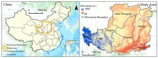
Figure 1.
Location of the Loess Plateau.
2.2. Data Sources
The data include land use data, digital elevation model data (DEM), soil data, net primary productivity data (NPP), evapotranspiration data (ET), normal difference of vegetation index (NDVI), and meteorological data (i.e., precipitation, temperature, and solar radiation) (Table 1). The rasterized meteorological data were interpolated from meteorological station data using ANUSPLIN software. The final spatial unit size for assessment was determined as 1 × 1 km. All data were projected into the China Geodetic Coordinate System 2000 Albers projection to ensure spatial matching consistency of the multi-source data.

Table 1.
Data sources.
2.3. Methods
2.3.1. Evaluation of Ecosystem Services
The environmental and geographical characteristics of the study area were examined, and three ecosystem service types were selected for a detailed evaluation of the study area, including net primary productivity (NPP), soil conservation (SC), and water yield (WY). These services were standardized between 0 and 1, respectively, due to their different units of measurement. The comprehensive ecosystem service (CES) was also calculated for the study area [6]. Table 2 contains a list of the precise calculation formulas and explanations for each ecosystem service.
where SES is the standardization of ESs, ESsmin is 5% of the cumulative value of ESs, and ESsmax is 95% of them. This study first standardized each ecosystem service in 2020. The same thresholds were then used for the other years of standardized ESs to analyze their changes.
Table 2.
The formulas for evaluating ESs.
2.3.2. Climate Factors
Precipitation, temperature, and solar radiation are important climate factors that maintain ecosystem stability. The water cycle influences the materials exchange and the energy transfer in ecosystems, temperature regulates the cycle of biological activity, and solar radiation is the main source of energy for ecosystem processes, such as plant photosynthesis and transpiration [19]. Three variables, the annual total precipitation (ATP), mean annual temperature (MAT), and total annual solar radiation (ASR), were chosen to investigate the impact of climate change on ESs. The ATP was obtained by summing the daily site data and the MAT was obtained by averaging the daily site data. More detail of the calculation procedure of ASR can be found in the literature [52,53].
2.3.3. Trend Analysis of Ecosystem Services
To observe the trends of ESs and climate factors, the least squares method was used as Equation (3).
where i represents year, is the linear trend value, is the value within the image of year i, is the representative value for year i, n is the total number of year, > 0 indicates an increasing temporal trend, < 0 indicates a decreasing temporal trend, and the F-test was used to test for significance [54].
2.3.4. Relationships among Ecosystem Services and Climate Factors
- (1)
- Correlation analysis
The correlation analysis was used to investigate the relationships among ESs and climate factors and the trade-offs and synergies between ESs. Positive correlation represents synergistic relationship and negative correlation represents trade-off relationship. The Spearman correlation analysis and the F-test were calculated in MATLAB (significant represents p < 0.05, non-significant represents p > 0.05) [55].
- (2)
- Elasticity coefficient
Precipitation, temperature, and solar radiation were calculated separately at 2% intervals as the means of their corresponding standardized ESs. The relationship between climate factors as the independent variable and ESs as the dependent variable was established. The inflection point of the elasticity coefficient (threshold point) was determined by analyzing the elasticity coefficients of the ESs and climate factors. The elasticity coefficient is the change in ESs per unit change in climate factors and characterizes the strength and efficiency of the impact of the independent variable. The elasticity coefficients were obtained by deriving a fitted function for climate factors and ESs [16]. The cubic polynomial regression has been widely used to fit their relationship. The threshold is the inflection point value of the elasticity coefficient (Equation (4)).
where EC is the elasticity coefficient, ESs represents the ecosystem services, and x is the climate factor.
3. Results
3.1. Spatial and Temporal Patterns of Climate Factors
The spatial distribution and trend for each climate factor from 2000 to 2020 are shown in Figure 2. For ATP, the annual average was high in the southeastern region and low in the northwestern region and change trend showed a significant increase (p < 0.05) in the southwest and central regions of study area. The distribution of solar radiation was opposite to that of ATP, which was high in the northwestern and low in the southeastern regions. The solar radiation in the southwestern region showed a significant decrease trend (p < 0.05). MAT was high in the south and low in the north, which was the highest in the valley plain, and lower in the higher altitudes of Qin ling Mountains and Qilian Mountains. In terms of annual average change, ATP increased from 385.82 mm and 503.95 mm and showed a significant increase trend (p < 0.05). MAT fluctuated between 7.98 °C and 9.08 °C, and ASR fluctuated between 5477 MJ/(m2) and 5921 MJ/(m2). The two-climate factors showed non-significant trends (p > 0.05).
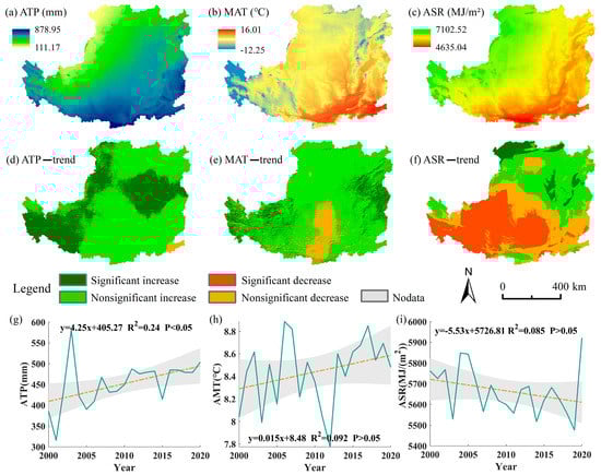
Figure 2.
Spatial distributions and temporal variations of climate factors (Note: (a–c) are multi-year average spatial distributions of climate factors; (d–f) are spatial trends in climate factors; (g–i) are annual average trends in climate factors).
3.2. Spatial and Temporal Variation in Ecosystem Services
The spatial distribution and trend for each ecosystem service from 2000 to 2020 are shown in Figure 3. In terms of spatial distribution, the differences among the various ESs were relatively considerable, and each ecosystem service had obvious spatial differentiation characteristics. NPP was high in the southeast and low in the northwest, and NPP in the south was significantly higher than other areas. The value of SC is larger in the higher altitude, which is caused by the high vegetation coverage and large slope in this region, and the value of WY is higher in the valley plain of the southeastern region and the grassland of the northern region. In the past 21 years, NPP and SC showed a significant increase in most areas, while WY showed a significant decreasing trend in the southeast (p < 0.05). In terms of annual average change, mean annual NPP increased from 213.03 gC/m2 to 355.07 gC/m2, and mean annual SC increased from 163.33 t/hm2 to 304.66 t/hm2. The two services showed significant increasing trend (p < 0.05) in the past 21 years. The mean annual WY fluctuated with a non-significant decreasing trend (p > 0.05) between 41.02 mm and 221.85 mm.
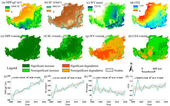
Figure 3.
Spatial distribution and temporal variation of ESs (Note: (a–d) are the multi-year average spatial distribution of ESs; (e–h) are the spatial trend of ESs; (i–l) are the average annual trend of ESs).
The relationships between ESs at pixles are shown in Figure 4. In terms of spatial distribution, NPP was synergistic with SC in 91.29% of the LP with 74.94% being significantly synergistic, while NPP was in a trade-off with WY in 72.93% of the area with a more significant trade-off in the southeast. The SC was synergistic with WY in 63.23% of the area, being more significant in the north (Table S1). In the southwestern hilly gullies, NPP and SC were in a trade-off with WY. Additionally, NPP and SC showed synergistic effects and WY showed trade-off effects with both NPP and SC for all pixles (see Table S2).
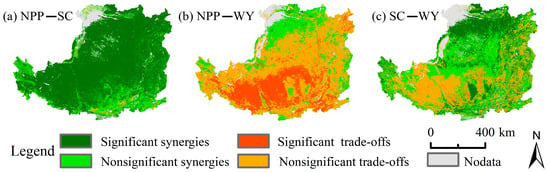
Figure 4.
Trade-offs and synergies between different ESs (Note: (a) is the relationship between NPP and SC; (b) is the relationship between NPP and WY; (c) is the relationship between SC and WY).
3.3. Correlation among Ecosystem Services and Climate Factors
The spatial correlations among ESs and climate factors from 2000 to 2020 are shown in Figure 5. ATP showed positive correlation with all ESs, and ASR showed negative correlation with all ESs. MAT was only positively correlated with NPP and negatively correlated with all other ESs (see Table S3). In terms of spatial distribution, NPP, SC, WY, and CES were all significantly positively correlated with changes in ATP, and the correlations for NPP and SC were stronger. The relationships of MAT on CES, NPP, SC, and WY were not significant in most regions. NPP was positively correlated with MAT in 70.64% but did not pass the significance test (p > 0.05), and 22.03% were not significantly negatively correlated (p > 0.05), particularly in the gully areas. There was 47.37% of SC that was not significantly positively correlated with MAT (p > 0.05), which were predominantly in LP gullies, and 50.83% of which were not significantly negatively correlated (p > 0.05). The response of WY to MAT was 91.47% negative, 11.44% of which was significantly negative. This was predominantly in the grassland and cropland areas in the western and northern parts of the LP. ASR had a significant negative influence on NPP and SC in the southern and central high-mountain forest areas of the LP (p < 0.05) (Table S4).
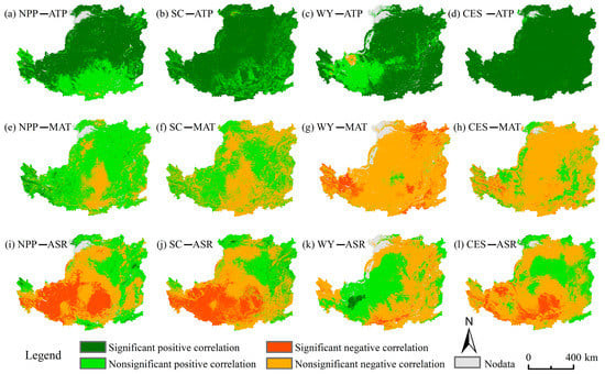
Figure 5.
Correlation among the ESs and the climate factors (Note: (a–d) are the spatial relationships among ESs and ATP; (e–h) are the spatial relationships among ESs and MAT; (i–l) are the spatial relationships among ESs and ASR).
3.4. Threshold Response of Ecosystem Services to Climate Factors
Variations in ESs and elasticity coefficients with ATP, MAT, and ASR are shown in Figure 6. The CES increased with increasing ATP and reached a maximum when ATP reached 1061 mm. The elasticity coefficients revealed that this process demonstrated an increasing and then decreasing elasticity coefficients curve. At 92 mm < ATP < 622 mm, the elasticity coefficient exhibited an upward trend with ATP increasing and driving the continued acceleration of CES. When ATP reached a threshold of 622 mm, the elasticity coefficient peaked at 0.0034, and ATP had the strongest effect on ESs. The CES fluctuated with MAT, with a positive correlation when MAT < 2.28 °C and 8.44 °C < MAT < 12.72 °C. There was a negative correlation when 2.28 °C < MAT < 8.44 °C and MAT > 12.72 °C, whereas the CES reached a maximum at MAT of 12.72 °C. The elasticity coefficient showed an initially decreasing and then increasing curve, which indicates that the MAT response intensity to CES decreased and then increased, with the threshold value occurring at MAT of 6.17 °C. The change in CES with ASR showed a fluctuating decreasing curve, with the elasticity coefficient showing a curve of decreasing and then increasing trend, reaching a minimum of −0.00037 at an ASR of 6071 MJ/(m2).
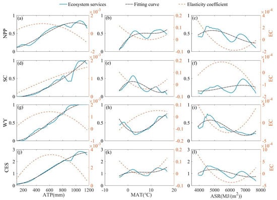
Figure 6.
Changes in the ESs, the elasticity coefficient and climate factors (Note: (a–c) are fitted curve for NPP with climate factors; (d–f) are the fitted curve for SC with climate factors; (g–i) are the fitted curve for WY with climate factors; (j–l) are the fitted curve for CES with climate factors).
The cubic polynomial fitting of ATP to ESs were the strongest (R2 > 0.9 see Table S5), and ATP continued to contribute to the growth of ESs. The promotion effect of ATP on NPP and WY declined after the 490 and 600 mm thresholds, respectively, when the elasticity coefficient reached its maximum. This indicates that the intensity of the effect of ATP on NPP and WY diminished after reaching these thresholds. The intensity of the effect of ATP on SC showed a continuous increase, meaning that the higher the ATP, the stronger the promotion effect. MAT promoted an increase in NPP and the intensity of this effect showed a weakening trend initially followed by strengthening. When MAT reached 9.19 °C, the elasticity coefficient reached the lowest value of −0.0021. Meanwhile, the promotion effect of MAT was the weakest. MAT had an inhibitory effect on SC, and the intensity of its effect also showed a trend of weakening initially and then strengthening. When MAT reached 7.90 °C, the elasticity coefficient reached its lowest value of 0.0373. ASR had a negative effect on NPP and WY, and the intensity of its effect first weakened and was then enhanced, with thresholds of 6302 MJ/(m2) and 5840 MJ/(m2), respectively. When the ASR was equal to the threshold value, the elasticity coefficient dropped to its lowest value of −0.00018 and 0.00028.
4. Discussion
4.1. Drivers of Climate Change on Ecosystem Services
As a primary part of terrestrial ecosystems, vegetation has an enormous impact on ESs [56]. Specifically, precipitation, temperature, and solar radiation have important effects on ESs since they are the key factors affecting vegetation growth, but their effects in the LP are slightly different (see Figure 5). Precipitation had a significant positive effect on ESs throughout the LP. With ATP increasing on a spatial scale, NPP, SC, and WY all showed a significant increase. Since a total of 73.7% of the LP is an arid and semi-arid region, the moisture becomes an important factor that limits vegetation growth. Temperature has a significant impact on ESs only in cold regions (approximately MAT < 2.2 °C). The NPP and SC showed an increasing trend with the increase in temperature, while WY showed a decreasing trend. Solar radiation had no significant effect on NPP and SC but significantly reduced WY. This is because higher solar radiation leads to stronger vegetation evapotranspiration [57]. In terms of temporal changes, the most significant impact of climate factors on ESs from 2000 to 2020 was ATP in the LP, while the impact of MAT and ASR on ESs was not obvious (see Figure 6). Similar results were obtained by Su et al. [35], and Sun et al. considered that there has been no significant change in temperature on the LP since 2000 under climate change [43]. This means that temperature has no remarkable effect on the ecosystem recovery of the LP. Overall, precipitation has a significant promoting effect on ESs of the LP and is favorable to the recovery of local ecosystems.
Despite the significant contribution of precipitation to ESs on the LP, the promotion of NPP and WY started to weaken when the ATP reached the 490 mm and 600 mm thresholds, respectively. The region at ATP > 490 mm mostly distributed in the southeastern part of the study area with cultivated land of the valley plains. The NPP of cultivated land is more prominently affected by strong artificial control (e.g., irrigation during drought). The region at ATP > 600 mm is mainly found in the southeast with the alpine woodlands and is relatively humid. Thus, moisture is not a limiting factor. The intensity of the effect of ATP on WY was weakened because of the high evapotranspiration caused by the high vegetation cover in this area [12,39,41]. It is worth noting that the promotive effect of precipitation on SC has been enhanced although the increase in precipitation potentially leads to increasing potential rainfall erosivity. However, the increase in the precipitation is greatly beneficial to the vegetation restoration and canopy interception capacity, which resulted in the increase in SC values [12].
Note that increasing precipitation does not necessarily increase CES. In other words, ESs do not always reach their maximum values under the same environmental conditions due to the trade-offs relationship among them. NPP and SC showed a synergistic relationship, while WY showed a trade-off relationship with NPP and SC. Precipitation may significantly promote vegetation recovery in LP, which can effectively contribute to enhancing carbon sequestration and the improvement of soil conservation [58]. However, the rapid growth of vegetation increases surface evapotranspiration resulting in decreasing WY [12,59]. Therefore, the balance among ESs should be emphasized to promote their improvement and maintain regional sustainable development. In future work, it is necessary to accurately assess the vegetation capacity of the LP and establish a new ecological protection model to reasonably guide regional management and development and avoid new ecological security problems.
4.2. Limitations and Applications
ESs are complex and diverse, but only NPP, SC, and WY were assessed. A range of ecosystem service types should be examined in future work, including biodiversity and habitat quality, to undertake a more detailed assessment of ESs. All meteorological data utilized were interpolated from meteorological stations data, which hampers accurate descriptions of complex climate change, despite our choice of a more accurate interpolation method. In future research, we will use local climate models to simulate climate change, with the aim of modeling the effects of climate change on ESs with greater precision [60,61].
More recent research has concentrated on the spatial and temporal distribution of ESs with less focus on the scale impacts of various communities. The driving thresholds for various environmental conditions have seldom been considered for a range of ESs. Threshold impacts of climate change on NPP, SC, WY, and CES were the primary focus, while the environmental context was considered. It is critical to balance ESs when recovering the LP to maximize the total ecosystem service supply. The results of this research offer a more thorough perspective for evaluating how ESs respond to climate change, not only in terms of determining the spatial heterogeneity of the effects of climate factors on various ESs and their threshold effects, but also in terms of offering a theoretical foundation and reference for the long-term sustainability of the LP ecosystem in the context of a changing climate. It also offers a crucial resource for maintaining the balance between ecological security patterns and human development on the LP.
5. Conclusions
Illustrations of the relationships between ESs and climate change are important prerequisites for supporting the sustainable development of the LP ecosystem. This study highlights significant influence of the precipitation on ESs, which has a facilitating effect. For NPP and WY, the facilitating effect of ATP weakens when ATP reaches thresholds of 490 mm and 600 mm, respectively. MAT has a facilitating effect on NPP and an inhibiting effect on SC, with the intensity of the effects both decreasing and then increasing, with inflection points of 9.19 °C and 7.90 °C. ASR had an inhibiting effect on NPP and WY, with the intensity of the effect weakening and then increasing with inflection points of 6302 MJ/(m2) and 5840 MJ/(m2). Under favorable precipitation conditions, NPP and SC tend to increase because the precipitation promotes significant local vegetation recovery. However, the higher the vegetation cover, the stronger the evapotranspiration, which ultimately led to a decreasing trend in WY. Researchers should strengthen climate change monitoring to respond appropriately to climate change whilst improving ecosystem services and maintaining ecosystem stability.
Supplementary Materials
The following supporting information can be downloaded at: https://www.mdpi.com/article/10.3390/f13122011/s1, Table S1: Proportion of trade-offs and synergies between ecosystem services; Table S2: Trade-offs and synergies for changes in ecosystem services; Table S3: Mean correlation (R) of ecosystem services and climate factors on the Loess Plateau; Table S4: Proportion of ecosystem services correlated with climate factors; Table S5: Three-fold fitted equations for ecosystem services and climate factors.
Author Contributions
P.J.: Investigation, Data curation, Visualization, Writing-original draft and Writing-review & editing. D.Z. (Donghai Zhang): Conceptualization, Methodology, Validation. Z.A.: Supervision, Validation. H.W.: Software, Visualization. D.Z. (Dingming Zhang): Data curation. H.R.: Investigation. L.S.: Visualization. All authors have read and agreed to the published version of the manuscript.
Funding
This work was supported by the Natural Science Foundation of Shaanxi Province (2021JQ563).
Conflicts of Interest
The authors declare that they have no known competing financial interests or personal relationships that could have appeared to influence the work reported in this paper.
References
- Costanza, R.; d’Arge, R.; de Groot, R.; Farber, S.; Grasso, M.; Hannon, B.; Limburg, K.; Naeem, S.; O’Neill, R.V.; Paruelo, J.; et al. The value of the world’s ecosystem services and natural capital. Nature 1997, 387, 253–260. [Google Scholar] [CrossRef]
- Liu, Y.; Fu, B.; Wang, S.; Zhao, W. Global ecological regionalization: From biogeography to ecosystem services. Environ. Sustain. 2018, 33, 1–8. [Google Scholar] [CrossRef]
- Vallet, A.; Locatelli, B.; Levrel, H.; Wunder, S.; Seppelt, R.; Scholes, R.J.; Oszwald, J. Relationships Between Ecosystem Services: Comparing Methods for Assessing Tradeoffs and Synergies. Ecol. Econ. 2018, 150, 96–106. [Google Scholar] [CrossRef]
- Wu, L.; Fan, F. Assessment of ecosystem services in new perspective: A comprehensive ecosystem service index (CESI) as a proxy to integrate multiple ecosystem services. Ecol. Indic. 2022, 138, 108800. [Google Scholar] [CrossRef]
- Fang, C.; Cai, Z.; Devlin, A.T.; Yan, X.; Chen, H.; Zeng, X.; Xia, Y.; Zhang, Q. Ecosystem services in conservation planning: Assessing compatible vs. incompatible conservation. J. Environ. Manag. 2022, 312, 114906. [Google Scholar] [CrossRef] [PubMed]
- Zhang, D.; Jing, P.; Sun, P.; Ren, H.; Ai, Z. The non-significant correlation between landscape ecological risk and ecosystem services in Xi’an Metropolitan Area, China. Ecol. Indic. 2022, 141, 109118. [Google Scholar] [CrossRef]
- Xu, Z.; Peng, J. Ecosystem services-based decision-making: A bridge from science to practice. Environ. Sci. Policy 2022, 135, 6–15. [Google Scholar] [CrossRef]
- Wu, X.; Liu, J.; Fu, B.; Wang, S.; Wei, Y.; Li, Y. Bundling regions for promoting Sustainable Development Goals. Environ. Res. Lett. 2022, 17, 44021. [Google Scholar] [CrossRef]
- Bai, Y.; Jiang, B.; Wang, M.; Li, H.; Alatalo, J.M.; Huang, S. New ecological redline policy (ERP) to secure ecosystem services in China. Land Use Policy 2016, 55, 348–351. [Google Scholar] [CrossRef]
- Zhang, J.; Mengting, L.; Hui, Y.; Xiyun, C.; Chong, F. Critical thresholds in ecological restoration to achieve optimal ecosystem services: An analysis based on forest ecosystem restoration projects in China. Land Use Policy 2018, 76, 675–678. [Google Scholar] [CrossRef]
- Wu, X.; Fu, B.; Wang, S.; Song, S.; Li, Y.; Xu, Z.; Wei, Y.; Liu, J. Decoupling of SDGs followed by re-coupling as sustainable development progresses. Nat. Sustain. 2022, 5, 452–459. [Google Scholar] [CrossRef]
- Fu, B.; Wang, S.; Liu, Y.; Liu, J.; Liang, W.; Miao, C. Hydrogeomorphic ecosystem responses to natural and anthropogenic changes in the Loess Plateau of China. Annu. Rev. Earth Planet. Sci. 2017, 45, 223–243. [Google Scholar] [CrossRef]
- Peng, J.; Tian, L.; Zhang, Z.; Zhao, Y.; Green, S.M.; Quine, T.A.; Liu, H.; Meersmans, J. Distinguishing the impacts of land use and climate change on ecosystem services in a karst landscape in China. Ecosyst. Serv. 2020, 46, 101199. [Google Scholar] [CrossRef]
- Chen, Y.; Feng, X.; Tian, H.; Wu, X.; Gao, Z.; Feng, Y.; Piao, S.; Lv, N.; Pan, N.; Fu, B. Accelerated increase in vegetation carbon sequestration in China after 2010: A turning point resulting from climate and human interaction. Glob. Chang. Biol. 2021, 27, 5848–5864. [Google Scholar] [CrossRef]
- Wang, L.; Ma, S.; Qiao, Y.; Zhang, J. Simulating the Impact of Future Climate Change and Ecological Restoration on Trade-Offs and Synergies of Ecosystem Services in Two Ecological Shelters and Three Belts in China. Environ. Res. Public Health 2020, 17, 7849. [Google Scholar] [CrossRef] [PubMed]
- Ma, S.; Wang, L.; Jiang, J.; Chu, L.; Zhang, J. Threshold effect of ecosystem services in response to climate change and vegetation coverage change in the Qinghai-Tibet Plateau ecological shelter. J. Clean. Prod. 2021, 318, 128592. [Google Scholar] [CrossRef]
- Akram, M.A.; Zhang, Y.; Wang, X.; Shrestha, N.; Malik, K.; Khan, I.; Ma, W.; Sun, Y.; Li, F.; Ran, J.; et al. Phylogenetic independence in the variations in leaf functional traits among different plant life forms in an arid environment. J. Plant Physiol. 2022, 272, 153671. [Google Scholar] [CrossRef]
- Akram, M.A.; Wang, X.; Hu, W.; Xiong, J.; Zhang, Y.; Deng, Y.; Ran, J.; Deng, J. Convergent Variations in the Leaf Traits of Desert Plants. Plants 2020, 9, 990. [Google Scholar] [CrossRef] [PubMed]
- Yao, S.; Akram, M.A.; Hu, W.; Sun, Y.; Sun, Y.; Deng, Y.; Ran, J.; Deng, J. Effects of Water and Energy on Plant Diversity along the Aridity Gradient across Dryland in China. Plants 2021, 10, 636. [Google Scholar] [CrossRef] [PubMed]
- Liu, D.; Wang, T.; Yang, T.; Yan, Z.; Liu, Y.; Zhao, Y.; Piao, S. Deciphering impacts of climate extremes on Tibetan grasslands in the last fifteen years. Sci. Bull. 2019, 64, 446–454. [Google Scholar] [CrossRef]
- Liu, L.; Jiang, Y.; Gao, J.; Feng, A.; Jiao, K.; Wu, S.; Zuo, L.; Li, Y.; Yan, R. Concurrent Climate Extremes and Impacts on Ecosystems in Southwest China. Remote Sens. 2022, 14, 1678. [Google Scholar] [CrossRef]
- Yin, L.; Dai, E.; Zheng, D.; Wang, Y.; Ma, L.; Tong, M. What drives the vegetation dynamics in the Hengduan Mountain region, southwest China: Climate change or human activity? Ecol. Indic. 2020, 112, 106013. [Google Scholar] [CrossRef]
- Kang, J.; Zhang, Y.; Biswas, A. Land Degradation and Development Processes and Their Response to Climate Change and Human Activity in China from 1982 to 2015. Remote Sens. 2021, 13, 3516. [Google Scholar] [CrossRef]
- Yan, H.; Du, W.; Feng, Z.; Yang, Y.; Xue, Z. Exploring adaptive approaches for social-ecological sustainability in the Belt and Road countries: From the perspective of ecological resource flow. J. Environ. Manag. 2022, 311, 114898. [Google Scholar] [CrossRef] [PubMed]
- Xiong, Q.; Xiao, Y.; Liang, P.; Li, L.; Zhang, L.; Li, T.; Pan, K.; Liu, C. Trends in climate change and human interventions indicate grassland productivity on the Qinghai–Tibetan Plateau from 1980 to 2015. Ecol. Indic. 2021, 129, 108010. [Google Scholar] [CrossRef]
- Yan, W.; He, Y.; Cai, Y.; Qu, X.; Cui, X. Relationship between extreme climate indices and spatiotemporal changes of vegetation on Yunnan Plateau from 1982 to 2019. Glob. Ecol. Conserv. 2021, 31, e1813. [Google Scholar] [CrossRef]
- Li, Y.; Piao, S.; Chen, A.; Ciais, P.; Li, L.Z.X. Local and teleconnected temperature effects of afforestation and vegetation greening in China. Natl. Sci. Rev. 2020, 7, 897–912. [Google Scholar] [CrossRef] [PubMed]
- Wu, G.L.; Cheng, Z.; Alatalo, J.M.; Zhao, J.; Liu, Y. Climate Warming Consistently Reduces Grassland Ecosystem Productivity. Earth’s Future 2021, 9, e2020EF001837. [Google Scholar] [CrossRef]
- Wang, C.; Vera-Vélez, R.; Lamb, E.G.; Wu, J.; Ren, F. Global pattern and associated drivers of grassland productivity sensitivity to precipitation change. Sci. Total Environ. 2022, 806, 151224. [Google Scholar] [CrossRef] [PubMed]
- Ji, S.; Ren, S.; Li, Y.; Fang, J.; Zhao, D.; Liu, J. The response of net primary productivity to climate change and its impact on hydrology in a water-limited agricultural basin. Environ. Sci. Pollut. Res. 2022, 29, 10277–10290. [Google Scholar] [CrossRef]
- Wang, Y.; Xiao, J.; Li, X.; Niu, S. Global evidence on the asymmetric response of gross primary productivity to interannual precipitation changes. Sci. Total Environ. 2022, 814, 152786. [Google Scholar] [CrossRef]
- Zheng, Z.; Zhu, W.; Chen, G.; Jiang, N.; Fan, D.; Zhang, D. Continuous but diverse advancement of spring-summer phenology in response to climate warming across the Qinghai-Tibetan Plateau. Agr. For. Meteorol. 2016, 223, 194–202. [Google Scholar] [CrossRef]
- Reich, P.B.; Bermudez, R.; Montgomery, R.A.; Rich, R.L.; Rice, K.E.; Hobbie, S.E.; Stefanski, A. Even modest climate change may lead to major transitions in boreal forests. Nature 2022, 608, 540–545. [Google Scholar] [CrossRef] [PubMed]
- Alkama, R.; Forzieri, G.; Duveiller, G.; Grassi, G.; Liang, S.; Cescatti, A. Vegetation-based climate mitigation in a warmer and greener World. Nat. Commun. 2022, 13, 1–10. [Google Scholar] [CrossRef] [PubMed]
- Su, C.; Fu, B. Evolution of ecosystem services in the Chinese Loess Plateau under climatic and land use changes. Glob. Planet. Change 2013, 101, 119–128. [Google Scholar] [CrossRef]
- Fu, B.; Wu, X.; Wang, Z.; Wu, X.; Wang, S. Coupling human and natural systems for sustainability: Experience from China’s Loess Plateau. Earth Syst. Dynam. 2022, 13, 795–808. [Google Scholar] [CrossRef]
- Feng, X.; Fu, B.; Piao, S.; Wang, S.; Ciais, P.; Zeng, Z.; Lü, Y.; Zeng, Y.; Li, Y.; Jiang, X.; et al. Revegetation in China’s Loess Plateau is approaching sustainable water resource limits. Nat. Clim. Chang. 2016, 6, 1019–1022. [Google Scholar] [CrossRef]
- Luo, Y.; Lü, Y.; Fu, B.; Zhang, Q.; Li, T.; Hu, W.; Comber, A. Half century change of interactions among ecosystem services driven by ecological restoration: Quantification and policy implications at a watershed scale in the Chinese Loess Plateau. Sci. Total Environ. 2019, 651, 2546–2557. [Google Scholar] [CrossRef] [PubMed]
- Wang, X.; Wu, J.; Liu, Y.; Hai, X.; Shanguan, Z.; Deng, L. Driving factors of ecosystem services and their spatiotemporal change assessment based on land use types in the Loess Plateau. J. Environ. Manag. 2022, 311, 114835. [Google Scholar] [CrossRef] [PubMed]
- Wu, X.; Wang, S.; Fu, B.; Feng, X.; Chen, Y. Socio-ecological changes on the Loess Plateau of China after Grain to Green Program. Sci. Total Environ. 2019, 678, 565–573. [Google Scholar] [CrossRef] [PubMed]
- Feng, X.; Li, J.; Cheng, W.; Fu, B.; Wang, Y.; Lü, Y.; Shao, M. Evaluation of AMSR-E retrieval by detecting soil moisture decrease following massive dryland re-vegetation in the Loess Plateau, China. Remote Sens. Environ. 2017, 196, 253–264. [Google Scholar] [CrossRef]
- Liang, Y.; Hashimoto, S.; Liu, L. Integrated assessment of land-use/land-cover dynamics on carbon storage services in the Loess Plateau of China from 1995 to 2050. Ecol. Indic. 2021, 120, 106939. [Google Scholar] [CrossRef]
- Sun, Q.; Miao, C.; Duan, Q.; Wang, Y. Temperature and precipitation changes over the Loess Plateau between 1961 and 2011, based on high-density gauge observations. Glob. Planet. Chang. 2015, 132, 1–10. [Google Scholar] [CrossRef]
- Wu, X.; Wei, Y.; Fu, B.; Wang, S.; Zhao, Y.; Moran, E.F. Evolution and effects of the social-ecological system over a millennium in China’s Loess Plateau. Sci. Adv. 2020, 6, eabc0276. [Google Scholar] [CrossRef] [PubMed]
- Runting, R.K.; Bryan, B.A.; Dee, L.E.; Maseyk, F.J.F.; Mandle, L.; Hamel, P.; Wilson, K.A.; Yetka, K.; Possingham, H.P.; Rhodes, J.R. Incorporating climate change into ecosystem service assessments and decisions: A review. Glob. Chang. Biol. 2017, 23, 28–41. [Google Scholar] [CrossRef] [PubMed]
- Gao, Y.; Zhou, X.; Wang, Q.; Wang, C.; Zhan, Z.; Chen, L.; Yan, J.; Qu, R. Vegetation net primary productivity and its response to climate change during 2001–2008 in the Tibetan Plateau. Sci. Total Environ. 2013, 444, 356–362. [Google Scholar] [CrossRef]
- Piao, S.; Fang, J.; Zhou, L.; Zhu, B.; Tan, K.; Tao, S. Changes in vegetation net primary productivity from 1982 to 1999 in China. Glob. Biogeochem. Cycles 2005, 19, GB2027. [Google Scholar] [CrossRef]
- Liu, H.; Zhang, A.; Liu, C.; Zhao, Y.; Zhao, A.; Wang, D. Analysis of the time-lag effects of climate factors on grassland productivity in Inner Mongolia. Glob. Ecol. Conserv. 2021, 30, e1751. [Google Scholar] [CrossRef]
- Jia, X.; Fu, B.; Feng, X.; Hou, G.; Liu, Y.; Wang, X. The tradeoff and synergy between ecosystem services in the Grain-for-Green areas in Northern Shaanxi, China. Ecol. Indic. 2014, 43, 103–113. [Google Scholar] [CrossRef]
- Zhao, M.; Peng, J.; Liu, Y.; Li, T.; Wang, Y. Mapping Watershed-Level Ecosystem Service Bundles in the Pearl River Delta, China. Ecol. Econ. 2018, 152, 106–117. [Google Scholar] [CrossRef]
- Peng, J.; Tian, L.; Liu, Y.; Zhao, M.; Hu, Y.; Wu, J. Ecosystem services response to urbanization in metropolitan areas: Thresholds identification. Sci. Total Environ. 2017, 607, 706–714. [Google Scholar] [CrossRef] [PubMed]
- Hay, J.E. Calculation of monthly mean solar radiation for horizontal and inclined surfaces. Sol. Energy 1979, 23, 301–307. [Google Scholar] [CrossRef]
- Rietveld, M.R. A new method for estimating the regression coefficients in the formula relating solar radiation to sunshine. Agric. For. Meteorol. 1978, 19, 243–252. [Google Scholar] [CrossRef]
- Wu, Y.; Tang, G.; Gu, H.; Liu, Y.; Yang, M.; Sun, L. The variation of vegetation greenness and underlying mechanisms in Guangdong province of China during 2001–2013 based on MODIS data. Sci. Total Environ. 2019, 653, 536–546. [Google Scholar] [CrossRef] [PubMed]
- Cao, S.; Zhang, L.; He, Y.; Zhang, Y.; Chen, Y.; Yao, S.; Yang, W.; Sun, Q. Effects and contributions of meteorological drought on agricultural drought under different climatic zones and vegetation types in Northwest China. Sci. Total Environ. 2022, 821, 153270. [Google Scholar] [CrossRef] [PubMed]
- Chong, J.; Haiyan, Z.; Zhidong, Z. Spatially explicit assessment of ecosystem services in China’s. Loess Plateau: Patterns, interactions, drivers, and implications. Glob. Planet. Chang. 2018, 161, 41–52. [Google Scholar]
- Akuraju, V.R.; Ryu, D.; George, B.; Ryu, Y.; Dassanayake, K. Seasonal and inter-annual variability of soil moisture stress function in dryland wheat field, Australia. Agr. For. Meteorol. 2017, 232, 489–499. [Google Scholar] [CrossRef]
- Feng, X.M.; Sun, G.; Fu, B.J.; Su, C.H.; Liu, Y.; Lamparski, H. Regional effects of vegetation restoration on water yield across the Loess Plateau, China. Hydrol. Earth Syst. Sci. 2012, 16, 2617–2628. [Google Scholar] [CrossRef]
- Zhang, L.; Fu, B.; Lü, Y.; Zeng, Y. Balancing multiple ecosystem services in conservation priority setting. Landsc. Ecol. 2014, 30, 535–546. [Google Scholar] [CrossRef]
- Stefanidis, S.P. Ability of different spatial resolution regional climate model to simulate air temperature in a forest ecosystem pf central Greece. Environ. Prot. Sustain. Dev. 2021, 22, 1488–1495. [Google Scholar]
- Olsson, J.; Berg, P.; Kawamura, A. Impact of RCM spatial resolution on the reproduction of local, subdaily precipitation. J. Hydrometeorol. 2015, 16, 534–547. [Google Scholar] [CrossRef]


Publisher’s Note: MDPI stays neutral with regard to jurisdictional claims in published maps and institutional affiliations. |
© 2022 by the authors. Licensee MDPI, Basel, Switzerland. This article is an open access article distributed under the terms and conditions of the Creative Commons Attribution (CC BY) license (https://creativecommons.org/licenses/by/4.0/).