Abstract
Because the two common tree species in Norway, Picea abies L. Karst (Norway spruce) and Pinus sylvestris L. (Scots pine), differ in their susceptibility to the fungus Heterobasidion spp., converting at least parts of the rot-infested spruce stands to pine pays-off economically in some cases. Pixel-level information on rot levels and site indexes (SI) across the stand are required to identify these cases to make decisions that increase the expected economic return of the stand. Applying the Value of Information (VoI) concept, we assessed the value of such information when choosing between planting spruce and pine on a clear-cut spruce stand. The VoIs were highest for the stands of medium–low dominant SI. There, the shift from spruce to pine in some pixels instead of planting spruce across the whole stand has the best-expected impact on the stand’s net present value. Additionally, planting densities are more often adjusted to the pixel SI in these dominant SIs. Given that the stand’s dominant SI is known, information on rot levels alone is more valuable than information on SI alone. The lower the interest rate in decision-making, the more the forest owner is willing to invest in information supporting forest management.
1. Introduction
Root and butt rot (RBR) is a disease caused by the pathogenic white-rot fungi Heterobasidion parviporum Niemelä and Korhonen and Heterobasidion annosum (Fr.) Bref. [1,2]. In Norway, such fungi mainly affect the coniferous tree species Norway spruce (Picea abies L. Karst) and Scots pine (Pinus sylvestris L.), causing significant economic losses. However, spruce and pine have different degrees of resistance against Heterobasidion spp. In Scots pine, the decay is typically restricted to the root system, although small patches of decay may occasionally rise a few decimetres above the root collar [3]. In Norway spruce, the decay column can reach up to 10–12 m in the stem [4]. Thus, it destroys the most valuable part of the tree, which is downgraded from sawn wood quality to pulpwood or energy wood, depending on the extent of decay.
A nationwide stump survey in 1992 showed that nearly every 5th harvested spruce in Norway had stem decay caused by Heterobasidion spp. [5]. That indicates that RBR represents a significant challenge to the long-term sustainability of forestry in Norway. Uncertainty over the presence and magnitude of RBR infection leads to poor management decisions [6], such as not harvesting at the economically optimal time [7] or not choosing the best tree species when regenerating a stand. That will increase economic losses.
Planting a species with low susceptibility to RBR can diminish the root rot problem and potentially free an infested site from inoculum over time [8]. However, the optimal choice of species depends on information about several parameters. For instance, the precise identification of site index (SI) and the magnitude of rot infection is essential for optimal forest management and species selection [9]. In Norway, the site index is defined as the dominant height for a given species at a given index age and expresses the productivity of an area [10,11]. Generally, in Fennoscandia, Scots pine performs better than spruce on poorer sites, whereas Norway spruce tends to grow better in richer sites [12,13,14]. At intermediate productive sites, the species selection is less straightforward [14]. However, depending on the presence and severity of RBR infestation on the site, it is sometimes also favourable to plant pine in areas normally more suitable for spruce [9].
The rot level (RL) refers to the share of RBR-infested stumps of the total amount of stumps in the previous generation of trees on a clear-felled site. The rot level drives the RBR transfer between the tree generations [2,15]. Although site fertility impacts tree growth, the rot level affects the value of wood at the end of the rotation [15].
In Norway, the site index is frequently estimated using aerial image interpretation in addition to field assessment and information obtained from previous inventories [16,17]. Airborne laser scanning methods combined with digital aerial photogrammetry are currently employed for site index estimation for better accuracy [17]. However, site index estimates still rank among the most error-prone data used in forest management planning [16,17], mostly due to the uncertainty regarding the current age estimation [18]. Regarding the presence of rot, there are few visible external symptoms in trees, making it hard to detect it visually. Recent studies have attempted to use areal imagery interpretation for identifying rot in spruce trees [19,20]. Better information on the presence of rot should also improve forest management decisions.
When facing uncertainty, the decision-maker may proceed based on currently available information or try to decrease the uncertainty by gathering new information [21]. In the case of selecting the tree species on a forest stand, obtaining accurate knowledge of the stand’s site index and the presence of RBR infection should improve the decision. However, it only pays off if the costs of acquiring this information are lower than the expected gains from better decisions. The Value of Information (VoI) analysis proposed by Raiffa and Schlaifer [22] is a commonly used tool for assessing if it is worth paying for new information. The VoI is a decision analysis tool for evaluating the potential value of additional information that enhances the estimate of alternative performances on one or more uncertain criteria [23]. VoI analysis can increase the robustness of the chosen alternative by leading decision-makers to collect information that reduces negative surprises [23,24]. That is especially important for decision-making in forestry, where actions such as selecting species or stand structure have long-term consequences and are often irreversible [25]. In the field of forest management, the VoI has been employed in various studies [21,24,26,27,28,29,30]. In this article, we add to this body of research by looking at the value of information in the context of tree species choices in the clear-cut Norway spruce stand under the possibility of RBR infection.
The objective of this study is to evaluate the value of having accurate information on the site indexes and rot levels in different locations (pixels) on the stand when the forest owner decides on species to plant on a clear-cut site previously dominated by spruce. Our hypothesis is that a clear-cut stand’s expected net present value (NPV) will increase if the decision on tree species (spruce or pine) is made at pixel level after acquiring accurate information on rot infection levels across the stand. Furthermore, we assume that the site index may include some variation across the dominant value, which is the average site index of the stand. We expected that information on this—i.e., the pixel level site indexes—is also relevant to the forest owner. For comparison, we also consider a case with a homogeneous site index (no variation assumed in the site index across the dominant site index). We will test these hypotheses by calculating the VoI for the above information. For all the cases, we estimate how much money a forest owner should, at maximum, be willing to pay to choose the ideal tree species without uncertainty.
2. Materials and Methods
2.1. Projecting the Stand Development Given the Initial RBR Level
We used the RotStand model [2] to simulate the stand development for the two main tree species of economic interest in Norway (Norway spruce and Scots pine), given the level of RBR infection on a previously spruce-dominated site. The reference area consists of a typical clear-cut stand where there were 900 stems per hectare (90% spruce and 10% pine) with a 30 cm mean stump diameter. In the case of RBR infection, we assumed the disease to have been on the site on average for 20 years before clear-cut. Harvest was assumed to have taken place during spring, followed by stump treatment which is one of the recently proposed forestry-related measures for climate change mitigation by the Norwegian government [31].
RotStand projects the spread of RBR in the trees and the volumes of rotten and healthy roundwood in the next rotation over time. For this study, we simulated scenarios with varying combinations of RL measured as a share of infested stumps in a pixel (0% to 100%) and SI (12 to 24 m) to predict future stand development. The planting density is adjusted according to the SI. To account for the cases where the pixel level site index is unknown and the decisions must be made using the dominant site index, we also simulated scenarios with the plant densities related to the plausible other site indexes. In Rotstand, the management of the stand affects the spread of Heterobasidion spp., which, in turn, affects the stand development, as explained by Möykkynen and Pukkala [32]. For more details on the Rotstand model, refer to Pukkala et al. [2].
2.2. Finding the Economically Optimal Tree Species
We assume the forest owner would use available information to maximise the stand’s expected NPV over infinity. The NPV consists of the discounted stumpage revenues from timber sales minus discounted silvicultural costs. Over an infinite amount of time, the NPV of the bare forest land is often called Land Expectation Value (LEV). The optimal tree species or combination of tree species is the one that gives the highest LEV for the stand (at the age that gives the highest LEV).
The formula of LEV is given in Equation (1). That gives the LEV in a discrete-time setting, where St refers to the stumpage value (EUR ha−1) at stand age t, I is the silvicultural costs (EUR ha−1), and r is the interest rate. Stumpage value St corresponds to the revenues minus operational costs of harvesting at age t. The first part of the formula contains the NPV of one rotation and the second part is a multiplier for the perpetual NPV.
We need data on roundwood prices, logging costs, and volume of roundwood assortments to calculate stumpage values (St). Roundwood prices are available for roadside in Norway. For them, we considered 49 EUR m−3 and 48 EUR m−3 for spruce and pine sawlogs, and 28 EUR m−3 and 27 EUR m−3 for spruce and pine pulpwood, respectively [33]. The rotten pulpwood was assumed to be worth 22 EUR m−3 for spruce and 21 EUR m−3 for pine. We employed the models of Dale et al. [34] and Eid [35] to estimate harvesting costs and Dale and Stamm [36] and Eid [35] for forwarding costs. Despite the fact that these models are relatively old, updating their hourly rates results in unit costs that are compatible with those currently observed in Norway. Volumes of sawlogs, pulpwood, and rotten pulpwood come from RotStand simulations. These data also disaggregate healthy and rotten wood. For silvicultural costs, our starting point was the average cost for planting spruce in 2021 from Statistics Norway [37]. We adjusted the costs according to the planted tree species and the number of seedlings per hectare determined by the stand’s dominant SI. Due to the Norwegian tax subsidy system, we deducted 35% of the planting costs accounting for the typical subsidies and tax benefits related to silvicultural activities (Skogfond). We used an interest rate of 3% for the baseline results and 2% for the sake of comparison.
2.3. Decision Trees and Data on Probabilities for VoI Analysis
The decision tree analysis helps to evaluate different management actions’ outcomes systematically [38]. We used decision trees for structuring the forest owners’ decision of species selection under uncertainty over rot levels on the stand while also considering uncertainty over site indexes in some cases.
We had data on 71 stands divided into 12,475 pixels of 16 m × 16 m from a case study area in Central and Eastern Norway. The shares of alternative rot level and site index distribution across the stand’s dominant site index were calculated from these data and used as probabilities in the decision trees.
We considered rot levels ranging from 0% to 100% in 5% intervals, for which the shares are displayed in Table 1. The harvest operator collected the data on the stumps. Overall, the average rot level of all stands corresponds well to the generally prevailing situation in Norway [5].

Table 1.
Distribution of the rot levels (RL). The rot level refers to the number of rotten stumps as a share of all stumps in the pixel. Source: own calculation based on stand data of the study area.
In addition to the case where we assumed a dominant site index X (X’s ranging from spruce SI 15 to 22) to prevail on the whole stand area (case “homogenous site index”), we accounted for the assumption supported by our dataset that some of the pixels in a stand are likely to be of different site indexes than the dominant one. Based on our dataset, we judged that the within-stand site index variation lies within X ± 2, X being the dominant site index. The distribution of such site index occurrences calculated from our dataset appears in Table 2.
Table 2.
Distribution of pixels across different site indexes (SI) in a stand whose dominant site index is X. Source: own calculation based on stand data of the study area.
The ex-ante VoI can be calculated according to Equation (2) [21,39], where x denotes the possible states of nature concerning the uncertain variables (rot level, site index), y denotes the possible messages from an information source (e.g., the realised rot level from the harvester data, improved site index information), the expected payoff of the optimal decision a without the additional information, and is the expected payoff of the optimal decision a given message y and state x, which is further averaged over all possible messages y. In other words, the VoI is calculated by comparing the expected LEV of the setup with more information with the setup with less information. The expected LEV should increase with more information and reduce with more uncertainty.
The decision trees (A–F) used in this study are presented in Table 3. They are divided into two groups: homogeneous and heterogenous areas regarding the site index’s uniformity. Each group’s first decision tree refers to the case with the least amount of information, serving as a baseline for comparisons within that group. We used the comparisons described in the last column to calculate the value of information of each parameter (rot level and site index) alone or combined. The following sections go over the decision trees in greater detail.
Table 3.
Decision trees and their classifications. Rot level and site index columns refer to the (un)certain component of each decision tree. The value of information column indicates the evaluated parameter, and next to it is the correspondent comparison. Items with a dash indicate no information on the relevant parameters and are considered the baseline for comparisons in either homogeneous or heterogenous site indexes.
2.3.1. Decision Trees for Homogenous and Known Site Index - Uncertainty about Rot Levels over the Stand Area
If the site index is known with certainty, but the forest owner does not know how possible rot is located over the stand area (i.e., on various pixels of the stands), Figure 1A displays the decision tree that the forest owner would use to decide on the optimal tree species on the stand under this case. Figure 1B illustrates the case when the forest owner first acquired the information on rot levels in the stand before making the planting decisions. By comparing the expected value of these two decision trees, we obtain the expected VoI on the rot level.
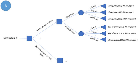

Figure 1.
Decision tree for homogeneous site index in all pixels when (A) rot levels are unknown and (B) rot levels are known. In (B), the decision is made after obtaining information on the rot level, while in (A) it is made before information is obtained. By comparing the outcomes of decision trees (A,B), one can obtain the value of information on rot level.
Without rot level knowledge, the decision to plant spruce or pine in the whole stand is based on the expected LEV obtained by summing up the LEVs of all rot level possibilities multiplied by their probability of occurrence (Figure 1A). The economically optimal choice is the species and harvesting age combination that gives the highest expected LEV at stand level. However, by acquiring information on the rot level on the various stand pixels, the forest owner can choose for each pixel the species that maximises its LEV under given harvesting age (Figure 1B). Again, the harvesting age with the highest expected LEV is economically optimal. In the first case, the decision-maker chooses the decision with the highest expected LEV at different rot levels. In contrast, in the second case, the decision-maker chooses the highest LEV separately for all the rot levels. The expected LEV is calculated across the set of pixel optimal decisions. The VoI on pixel-specific rot levels in a stand is determined by the expected improvement in the LEV when the planting decision is made after possessing the rot level information (decision tree B) compared to the case where the decision is made without it (decision tree A).
2.3.2. Decision Trees for Heterogeneous Site Index - Uncertainty about Rot Levels and Site Index over the Stand Area
The stands typically consist of pixels of their dominant site index and higher or lower site productivity than the dominant one (Table 2). The theoretical framework (Figure 2) used to determine the value of rot level and site index information in those areas starts by assuming the forest owner only knows the stand’s dominant site index while being aware of its spatial variation.
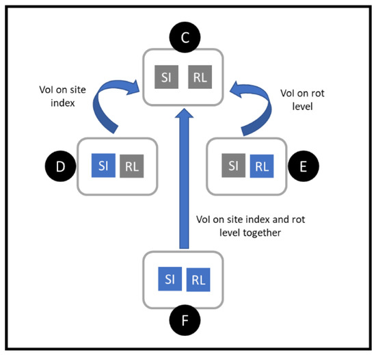
Figure 2.
Theoretical framework for calculating the Value of Information in areas of heterogeneous site indexes. SI refers to site index and RL to rot level. The grey square means that information on that parameter is unknown, while the blue square means that the parameter is known. The decision trees are labelled with the letters C-F help so that the reader knows which one we are referring to. The comparisons we made between decision tree outcomes to derive each value of information (VoI) are indicated with blue arrows.
If the forest owner does not know the site index or the amount of rot at the pixel level, he/she must make the planting decision under the conditions illustrated by decision tree C. After acquiring information on site indexes, the forest owner can adjust the plant density and tree species at the pixel level (decision tree D). By comparing the outcomes of decision trees D and C, we obtain the value of information on site index. If the forest owner decides to obtain information on rot level, he/she makes the planting decision under the conditions depicted by decision tree E. We can assess the benefit of acquiring information on rot levels by comparing the expected LEV obtained with decision trees E and C. However, if the forest owner decides to acquire information on both rot level and site index parameters, the planting decision will follow decision tree F. In this case, the value of information on both parameters is determined by comparing the expected LEV of decision trees F and C.
Figure 3, Figure 4, Figure 5 and Figure 6 display the decision trees used to solve the setups described in Figure 2.
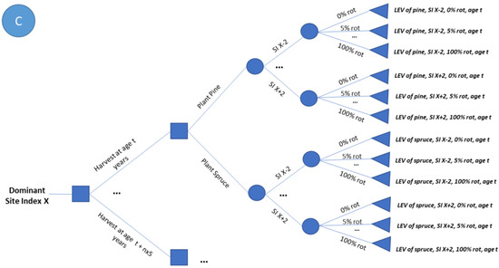
Figure 3.
Decision tree “C” for cases where site indexes and rot levels are unknown at pixel level before planting decision (see also Figure 2). This case is the baseline for calculating the value of information on rot level, site indexes and both parameters together. X refers to the dominant site index of the stand. Rot levels vary from 0–100 with 5% intervals. Harvest ages t alternate from t = 40 to t = 100 years with 5-year intervals (n = 0–12).
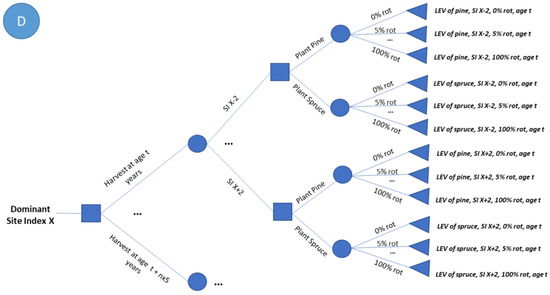
Figure 4.
Decision tree “D” for cases where rot levels are unknown, but site indexes are known at the pixel level before planting decision (see Figure 2). Here, the decision is made after obtaining information on site index, so the appropriate plant density is used. By comparing its outcome with decision tree C, one can obtain the value of information on site index. X refers to the dominant site index of the stand. Rot levels vary from 0–100 with 5% intervals. Harvest ages t alternate from t = 40 to t = 100 years with 5-year intervals (n = 0–12).
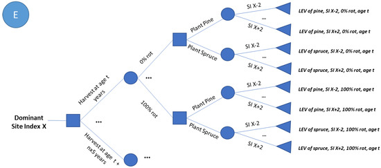
Figure 5.
Decision tree “E” for cases where the site indexes are unknown, but the rot levels are known at pixel level before planting decision (see also Figure 2). Here, the decision is made after obtaining information on rot level. By comparing its outcome with decision tree C, one can obtain the value of information on rot level. X refers to the dominant site index of the stand. Rot levels vary from 0–100 with 5% intervals. Harvest ages t alternate from t = 40 to t = 100 years with 5-year intervals (n = 0–12).
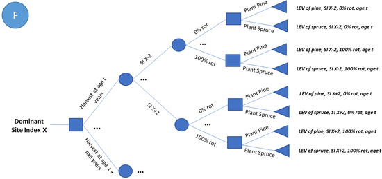
Figure 6.
Decision tree “F” for cases where both site indexes and rot levels are known before planting decision (see also Figure 2). Here, the decision is made after obtaining information on rot level and site index. By comparing its outcome with decision tree C, one can obtain the value of information on rot level and site index together. X refers to the dominant site index of the stand. Rot levels vary from 0–100 with 5% intervals. Harvest ages t alternate from t = 40 to t = 100 years with 5-year intervals (n = 0–12).
3. Results
3.1. Value of Information of Rot Levels When the Site Index Is Known and Homogenous
Figure 7 shows the values of information on rot levels for areas with homogeneous site index. With an interest rate of 3% and given the other assumptions considered in this study, the VoI varies from 1% to 37% of the expected LEV obtained without information on rot level (in absolute terms 35 EUR ha−1 to 98 EUR ha−1). Reducing the interest rate from 3% to 2% increases the absolute value of VoI, as can be expected. However, because the expected LEV increases considerably when the interest rate decreases from 3% to 2%, the relative VoI is smaller in the latter case, especially in the stands with a low dominant site index.
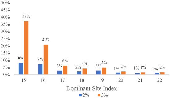
Figure 7.
Value of Information (VoI) of rot level relative to the expected land expectation value (LEV) obtained when deciding on the tree species to plant without information on the rot level. The values are for areas of homogeneous site index known by the owner, under interest rates of 2% and 3%.
The VoI varies across site indexes, with a tendency to decrease as the site index increases. The VoI appears to be at its highest around the stands with the lowest SIs (SI 15 and SI 16) considered in this study.
3.2. Value of Information on Rot Levels and Site Indexes When the Stand Has Heterogenous Site Index Structure
3.2.1. Acquiring Information on Rot Levels Only
For a 3% interest rate, the VoI of rot levels ranges from 1% to 39% of the expected LEV without the information (Figure 8). In absolute terms, the VoI ranges from 35 EUR ha−1 to 76 EUR ha−1 depending on the dominant site index of the stand. For 2% interest rates, the VoI ranges from 1% to 8% when measured as a share of LEV, the equivalent of 69 EUR ha−1 to 167 EUR ha−1. The benefits of acquiring information on rot levels are again highest at dominant site indexes 15 and 16. These stands consist of pixels of site indexes where the shift from spruce to pine is triggered by lower and, thus, more frequently occurring rot levels than what is the case with the higher site indexes.
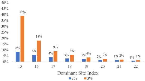
Figure 8.
Value of Information (VoI) of rot level relative to the expected land expectation value (LEV) obtained when deciding on the tree species to plant without information on the rot level. The values are for areas with heterogeneous site indexes under 2% and 3% interest rates.
3.2.2. Acquiring Information on Site Indexes Only
When comparing the expected LEVs of decision trees with and without information (D–C), one can notice that the exact information on site indexes across the stands with the highest dominant site indexes is likely not helpful. Figure 9 shows that on the lowest site indexes, the VoI for 3% interest rate is at the highest 14% of the expected LEV with information on the dominant site index only (27 EUR ha−1 in absolute terms).
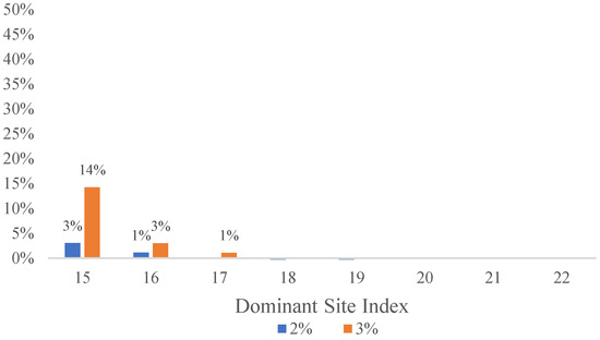
Figure 9.
Value of Information (VoI) of site index relative to the expected land expectation value (LEV) obtained when deciding on the tree species to plant without information on the site index. The values are for areas with heterogeneous site indexes under 2% and 3% interest rates.
3.2.3. Information on Both Rot Levels and Site Indexes
The VoI of both rot level and site index parameters indicates again that the lower the dominant site index (among the site indexes considered in this study), the more the forest owner should be willing to pay for information on site indexes and rot levels (Figure 10a). For the 3% interest rate, the VoI reaches up to 47% of the expected LEV without information (equivalent to 90 EUR ha−1). The VoI is affected by both site index and rot level information at low site indexes, whereas at high site indexes, almost all of the expected gain from information comes from rot level information alone. Overall, the VoI reduces as the dominant site index increases. Figure 10b compares the VoI for each parameter separately (when the other is unknown) and combined under an interest rate of 3%.

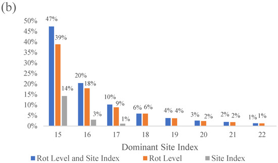
Figure 10.
(a) Value of Information (VoI) of site index and rot level relative to the expected land expectation value (LEV) obtained when deciding on the tree species to plant without information on both site index and rot level. The values are for areas with heterogeneous site indexes under 2% and 3% interest rates. (b) VoI of site index + rot level; rot level only; and site index only under an interest rate of 3%.
4. Discussion
The results indicate that acquiring information on rot levels is worthwhile to reduce the decision-makers uncertainty when selecting the tree species for regenerating spruce stands in Norway.
Pixel level information on rot levels is more important than pixel level information on site index when the dominant site index of the stand is already known. The former yields the highest returns when its uncertainty is resolved (Figure 10b). The VoI appears to be at its highest around the stands with the lowest site indexes considered in this study (SI 15 and SI 16), for areas of both homogeneous and heterogeneous site indexes. A relatively low threshold is observed for these site indexes for shifting the optimal tree species to pine in the presence of rot (15%). Such low rot levels occur more frequently than the higher ones (see Table 1) that are required to make the shift from spruce to pine advantageous at the higher site indexes. Therefore, the rot level information will more frequently have a positive impact on the LEV of these site indexes. Spruce is an economically better choice in areas with a higher dominant site index and RL up to 35%. That is due to the vigorous growth of spruce vs. lower pine growth in high productivity sites, compensating for losses caused by RBR [9].
Our study indicates that exact information on site indexes across stands with the highest dominant site indexes (SI ≥ 18) is likely not helpful. That is because in our study setting there is little variation in planting densities across the expected site index range in the stand (SI ± 2) (Figure 9). Hence, the information on the pixel level site index does not change the forest owner’s decision on planting. However, it is likely to be worthwhile to acquire information on this parameter in areas with medium-low dominant SI (15 and 16) where there is variation in planting density across the dominant and its neighbouring site indexes. If the forest owner only knows the dominant site index, he/she will use the same plant density across the whole stand. Instead, information about pixel-level site indexes allows pixel-by-pixel adjustment on the plant densities and possibly tree species, as Table A1 in Appendix A shows a prevalence of pine in low site indexes and spruce in high site indexes.
Regarding Figure 9, we should point out that the relative VoI for stands of dominant SIs 17–19 were calculated to be slightly negative (−0.1% to −1.1% of LEV) when using a 2% interest rate. That is due to the simplification in our calculations which considered the same plant density for both simulations with 2% and 3% interest rates. When the site index is known, the plant density can be adjusted at the pixel level, while in the lack of information, densities of the dominant site indexes are employed in the calculation. However, we used the recommended densities that might not be ideal for a 2% interest rate, while they seemed to work out well for the 3% case. Ideally, however, one should compare the cases using the optimal plant densities for 2%. Since the VoI cannot be negative and the differences were caused by dissimilar decision options, the best solution for trees C and D can be assumed to be the correct optimum. Consequently, the negative VoIs were set to zero.
The VoI, which is the amount an individual is willing to pay at maximum to be able to decide without uncertainty, is overall at highest when we obtain information on both rot level and site index. Yet, the marginal value of knowing the accurate site index at the pixel level is often low.
5. Conclusions
Acquiring information on site indexes and rot levels across the various locations (pixels) on the stand reduces the uncertainty faced by a forest owner selecting the tree species for stand regeneration. The maximum amount a forest owner should be willing to pay for information to reduce uncertainty, known as the Value of Information, varies according to the interest rate used in forest management and the dominant site index of the spruce stands we studied.
As expected, pixel-level knowledge on both site indexes and rot levels across the forest stand has higher VoI than respective knowledge of either rot levels or site indexes alone. Given our assumptions on prices and silvicultural costs, the forest owner who applies a 3% interest rate could pay for this information up to 1–47% (36 EUR ha−1 to 90 EUR ha−1) of the LEV expected to be obtained when choosing the tree species to plant without this information. The large variation is related to the alternative dominant site indexes of the stands. If one must choose only one of these two parameters to acquire pixel-level information on, that should be the rot levels for which the VoI ranges from 1% to 39% of the expected LEV without information. Information on specific rot levels across the stand improves the expected outcome of the decision regardless of the stand’s dominant site index. Instead, given that its dominant site index is known, pixel-level information on site indexes across the stand is likely irrelevant for the highest dominant site indexes. That is because, in the cases of high site indexes, spruce is always preferred if the accurate rot levels are unknown and planting densities are not affected by small site-index variation in the neighbourhood of the dominant site index.
Overall, we obtained the highest VoIs in medium-low site index stands. The option for deciding the shift from spruce to pine on pixel level has the best-expected impact on LEV in such stands. In higher dominant spruce site indexes, the VoI becomes lower. Not only is the pixel-level site index information less relevant in high-site index stands, but the pixels with high enough rot levels to make the shift from spruce to pine pay off in such stands are not common.
The interest rate the forest owner applies in forest management plays an essential role in determining the VoI. The lower the interest rate in decision-making, the more willing the forest owner is to invest in forest management and information supporting it. Accordingly, the value of information on rot levels and site indexes across the stand is higher, with an interest rate of 2% than 3%. However, in relative terms, when VoI is expressed as a share of LEV expected to be obtained without acquiring additional information, VoI was higher for an interest rate of 3% than for 2% in our results. That is due to the much higher expected LEV used for comparison in the latter, 2% case.
Author Contributions
Conceptualisation, A.A., A.K. and A.M.I.K.; methodology, A.A., A.K. and A.M.I.K.; software, A.A.; validation, A.K. and A.M.I.K.; formal analysis, A.A., A.K. and A.M.I.K.; investigation, A.A.; resources, A.M.I.K.; data curation, A.A. and A.M.I.K.; writing—original draft preparation, A.A.; writing—review and editing, A.A., A.K. and A.M.I.K.; visualisation, A.A.; supervision, A.K. and A.M.I.K.; project administration, A.M.I.K. All authors have read and agreed to the published version of the manuscript.
Funding
This research was funded by The Research Council of Norway through the PRECISION project—Precision forestry for improved resource use and reduced wood decay in Norwegian Forests (project number NFR281140).
Data Availability Statement
The datasets generated/analysed during the current study are available from the corresponding author upon reasonable request.
Conflicts of Interest
The authors declare no conflict of interest.
Appendix A
Table A1.
Optimal tree species to plant for each combination of site index, initial rot level, and rotation length. P stands for Pinus sylvestris (pine) and S for Picea abies (spruce) for a planted forest. The economically optimal rotation age (NPV based considering an interest rate of 3%) for each site index given a homogenous rot level is indicated in bold. Brackets indicate the negative NPVs.
| H40 SI | Rotation | Initial Rot Level (%) | ||||||||||||||||||||
|---|---|---|---|---|---|---|---|---|---|---|---|---|---|---|---|---|---|---|---|---|---|---|
| 0 | 5 | 10 | 15 | 20 | 25 | 30 | 35 | 40 | 45 | 50 | 55 | 60 | 65 | 70 | 75 | 80 | 85 | 90 | 95 | 100 | ||
| 13 | 55–70 | (P) | (P) | (P) | (P) | (P) | (P) | (P) | (P) | (P) | (P) | (P) | (P) | (P) | (P) | (P) | (P) | (P) | (P) | (P) | (P) | (P) |
| 13 | 75 | P | P | P | (P) | (P) | (P) | (P) | (P) | (P) | (P) | (P) | (P) | (P) | (P) | (P) | (P) | (P) | (P) | (P) | (P) | (P) |
| 13 | 80 | P | P | (P) | (P) | (P) | (P) | (P) | (P) | (P) | (P) | (P) | (P) | (P) | (P) | (P) | (P) | (P) | (P) | (P) | (P) | (P) |
| 13 | 85 | (S) | (P) | (P) | (P) | (P) | (P) | (P) | (P) | (P) | (P) | (P) | (P) | (P) | (P) | (P) | (P) | (P) | (P) | (P) | (P) | (P) |
| 13 | 90 | (S) | (S) | (P) | (P) | (P) | (P) | (P) | (P) | (P) | (P) | (P) | (P) | (P) | (P) | (P) | (P) | (P) | (P) | (P) | (P) | (P) |
| 14 | 55 | (P) | (P) | (P) | (P) | (P) | (P) | (P) | (P) | (P) | (P) | (P) | (P) | (P) | (P) | (P) | (P) | (P) | (P) | (P) | (P) | (P) |
| 14 | 60–65 | (S) | (P) | (P) | (P) | (P) | (P) | (P) | (P) | (P) | (P) | (P) | (P) | (P) | (P) | (P) | (P) | (P) | (P) | (P) | (P) | (P) |
| 14 | 70 | S | (S) | (P) | (P) | (P) | (P) | (P) | (P) | (P) | (P) | (P) | (P) | (P) | (P) | (P) | (P) | (P) | (P) | (P) | (P) | (P) |
| 14 | 75 | S | S | P | (P) | (P) | (P) | (P) | (P) | (P) | (P) | (P) | (P) | (P) | (P) | (P) | (P) | (P) | (P) | (P) | (P) | (P) |
| 14 | 80 | S | S | S | (P) | (P) | (P) | (P) | (P) | (P) | (P) | (P) | (P) | (P) | (P) | (P) | (P) | (P) | (P) | (P) | (P) | (P) |
| 14 | 85 | S | S | S | (P) | (P) | (P) | (P) | (P) | (P) | (P) | (P) | (P) | (P) | (P) | (P) | (P) | (P) | (P) | (P) | (P) | (P) |
| 14 | 90 | S | S | (S) | (S) | (P) | (P) | (P) | (P) | (P) | (P) | (P) | (P) | (P) | (P) | (P) | (P) | (P) | (P) | (P) | (P) | (P) |
| 15 | 55 | (P) | (P) | (P) | (P) | (P) | (P) | (P) | (P) | (P) | (P) | (P) | (P) | (P) | (P) | (P) | (P) | (P) | (P) | (P) | (P) | (P) |
| 15 | 60 | S | (P) | (P) | (P) | (P) | (P) | (P) | (P) | (P) | (P) | (P) | (P) | (P) | (P) | (P) | (P) | (P) | (P) | (P) | (P) | (P) |
| 15 | 65–70 | S | S | P | P | P | P | P | P | P | P | P | P | P | P | P | P | P | P | P | P | P |
| 15 | 75 | S | S | S | P | P | P | P | P | P | P | P | P | P | P | P | P | P | P | P | P | P |
| 15 | 80 | S | S | S | P | P | P | P | P | P | P | P | P | P | P | P | P | P | P | P | P | P |
| 15 | 85–90 | S | S | S | S | P | P | P | P | P | P | P | P | P | P | P | P | P | P | P | P | P |
| 16 | 55 | S | P | P | P | P | P | (P) | (P) | (P) | (P) | (P) | (P) | (P) | (P) | (P) | (P) | (P) | (P) | (P) | (P) | (P) |
| 16 | 60–65 | S | S | P | P | P | P | P | P | P | P | P | P | P | P | P | P | P | P | P | P | P |
| 16 | 70 | S | S | S | P | P | P | P | P | P | P | P | P | P | P | P | P | P | P | P | P | P |
| 16 | 75 | S | S | S | P | P | P | P | P | P | P | P | P | P | P | P | P | P | P | P | P | P |
| 16 | 80 | S | S | S | P | P | P | P | P | P | P | P | P | P | P | P | P | P | P | P | P | P |
| 16 | 85–90 | S | S | S | S | P | P | P | P | P | P | P | P | P | P | P | P | P | P | P | P | P |
| 17 | 55 | S | S | S | S | P | P | (P) | (P) | (P) | (P) | (P) | (P) | (P) | (P) | (P) | (P) | (P) | (P) | (P) | (P) | (P) |
| 17 | 60–65 | S | S | S | S | S | P | P | P | P | P | P | P | P | P | P | P | P | P | P | P | P |
| 17 | 70 | S | S | S | S | S | P | P | P | P | P | P | P | P | P | P | P | P | P | P | P | P |
| 17 | 75 | S | S | S | S | S | P | P | P | P | P | P | P | P | P | P | P | P | P | P | P | P |
| 17 | 80 | S | S | S | S | S | P | P | P | P | P | P | P | P | P | P | P | P | P | P | P | P |
| 17 | 85–90 | S | S | S | S | S | S | P | P | P | P | P | P | P | P | P | P | P | P | P | P | P |
| 18 | 55–65 | S | S | S | S | S | P | P | P | P | P | P | P | P | P | P | P | P | P | P | P | P |
| 18 | 70 | S | S | S | S | S | S | P | P | P | P | P | P | P | P | P | P | P | P | P | P | P |
| 18 | 75 | S | S | S | S | S | S | P | P | P | P | P | P | P | P | P | P | P | P | P | P | P |
| 18 | 80–90 | S | S | S | S | S | S | P | P | P | P | P | P | P | P | P | P | P | P | P | P | P |
| 19 | 55–65 | S | S | S | S | S | P | P | P | P | P | P | P | P | P | P | P | P | P | P | P | P |
| 19 | 70 | S | S | S | S | S | P | P | P | P | P | P | P | P | P | P | P | P | P | P | P | P |
| 19 | 75 | S | S | S | S | S | P | P | P | P | P | P | P | P | P | P | P | P | P | P | P | P |
| 19 | 80–90 | S | S | S | S | S | S | P | P | P | P | P | P | P | P | P | P | P | P | P | P | P |
| 20 | 55–60 | S | S | S | S | S | S | P | P | P | P | P | P | P | P | P | P | P | P | P | P | P |
| 20 | 65 | S | S | S | S | S | S | S | P | P | P | P | P | P | P | P | P | P | P | P | P | P |
| 20 | 70 | S | S | S | S | S | S | S | P | P | P | P | P | P | P | P | P | P | P | P | P | P |
| 20 | 75–90 | S | S | S | S | S | S | S | P | P | P | P | P | P | P | P | P | P | P | P | P | P |
| 21 | 55–60 | S | S | S | S | S | S | S | P | P | P | P | P | P | P | P | P | P | P | P | P | P |
| 21 | 65 | S | S | S | S | S | S | S | P | P | P | P | P | P | P | P | P | P | P | P | P | P |
| 21 | 70 | S | S | S | S | S | S | S | P | P | P | P | P | P | P | P | P | P | P | P | P | P |
| 21 | 75–85 | S | S | S | S | S | S | S | S | P | P | P | P | P | P | P | P | P | P | P | P | P |
| 21 | 90 | S | S | S | S | S | S | S | P | P | P | P | P | P | P | P | P | P | P | P | P | P |
| 22 | 55–60 | S | S | S | S | S | S | S | P | P | P | P | P | P | P | P | P | P | P | P | P | P |
| 22 | 65 | S | S | S | S | S | S | S | P | P | P | P | P | P | P | P | P | P | P | P | P | P |
| 22 | 70–75 | S | S | S | S | S | S | S | P | P | P | P | P | P | P | P | P | P | P | P | P | P |
| 22 | 80 | S | S | S | S | S | S | S | S | P | P | P | P | P | P | P | P | P | P | P | P | P |
| 22 | 85–90 | S | S | S | S | S | S | S | P | P | P | P | P | P | P | P | P | P | P | P | P | P |
| 23 | 55–60 | S | S | S | S | S | S | S | S | P | P | P | P | P | P | P | P | P | P | P | P | P |
| 23 | 65 | S | S | S | S | S | S | S | S | P | P | P | P | P | P | P | P | P | P | P | P | P |
| 23 | 70 | S | S | S | S | S | S | S | S | P | P | P | P | P | P | P | P | P | P | P | P | P |
| 23 | 75–80 | S | S | S | S | S | S | S | S | S | P | P | P | P | P | P | P | P | P | P | P | P |
| 23 | 85 | S | S | S | S | S | S | S | S | P | P | P | P | P | P | P | P | P | P | P | P | P |
| 23 | 90 | S | S | S | S | S | S | S | P | P | P | P | P | P | P | P | P | P | P | P | P | P |
| 24 | 55 | S | S | S | S | S | S | S | S | P | P | P | P | P | P | P | P | P | P | P | P | P |
| 24 | 60 | S | S | S | S | S | S | S | S | P | P | P | P | P | P | P | P | P | P | P | P | P |
| 24 | 65 | S | S | S | S | S | S | S | S | P | P | P | P | P | P | P | P | P | P | P | P | P |
| 24 | 70–80 | S | S | S | S | S | S | S | S | P | P | P | P | P | P | P | P | P | P | P | P | P |
| 24 | 85–90 | S | S | S | S | S | S | S | P | P | P | P | P | P | P | P | P | P | P | P | P | P |
References
- Woodward, S.; Stenlid, J.; Karjalainen, R.; Hûtterman, A. Heterobasidion Annosum: Biology, Ecology, Impact, and Control; CAB International: Wallingford, UK; New York, NY, USA, 1998. [Google Scholar]
- Pukkala, T.; Möykkynen, T.; Thor, M.; Rönnberg, J.; Stenlid, J. Modeling infection and spread of Heterobasidion annosum in even-aged Fennoscandian conifer stands. Can. J. For. Res. 2005, 35, 74–84. [Google Scholar] [CrossRef]
- Laine, L. The occurrence of Heterobasidion annosum (Fr.) Bref. in woody plants in Finland. Commun. Inst. For. Fenn. 1976, 90, 53. [Google Scholar]
- Stenlid, J.; Wästerlund, I. Estimating the frequency of stem rot in Picea abies using an increment borer. Scand. J. For. Res. 1986, 1, 303–308. [Google Scholar] [CrossRef]
- Huse, K.J.; Solheim, H.; Venn, K. Råte i Gran Registrert på Stubber Etter Hogst Vinteren 1992 [Rot in Spruce Registered at Stumps after Harvesting at Winter 1992]. In Rapport fra Skogforskningen; Norwegian Forest Research Institute-NIBIO: Ås, Norway, 1994. [Google Scholar]
- Hylen, G.; Granhus, A. A probability model for root and butt rot in Picea abies derived from Norwegian national forest inventory data. Scand. J. For. Res. 2018, 33, 657–667. [Google Scholar] [CrossRef]
- Aza, A.; Kangas, A.; Gobakken, T.; Kallio, A.M.I. Effect of root and butt rot uncertainty on optimal harvest schedules and expected incomes at the stand level. Ann. For. Sci. 2021, 78, 11p. [Google Scholar] [CrossRef]
- Korhonen, K.; Delatour, C.; Greig, B.J.W.; Sconhar, S. Silvicultural Control. In Heterobasidion Annosum: Biology, Ecology, Impact and Control; CAB International: Wallingford, UK; New York, NY, USA, 1998; pp. 283–313. [Google Scholar]
- Aza, A.; Kallio, A.M.I.; Pukkala, T.; Hietala, A.; Gobakken, T.; Astrup, R. Species selection in areas subjected to risk of root and butt rot: Applying Precision forestry in Norway. Silva Fenn. 2022, 56. [Google Scholar] [CrossRef]
- Tveite, B. Bonitetskurver for Gran [Site-Index Curves for Norway Spruce (Picea abies (L.) Karst)]; Norwegian Forest Research Institute-NIBIO: Ås, Norway, 1977; pp. 1–84. [Google Scholar]
- Hägglund, B.; Lundmark, J. Handledning i Bonitering Med Skogshögskolans Boniteringssystem [Guide in Using Site Index System According to the Swedish Forest School]; National Board of Forestry: Jönköping, Sweden, 1981; p. 124. [Google Scholar]
- Bielak, K.; Dudzińska, M.; Pretzsch, H. Mixed stands of Scots pine (Pinus sylvestris L.) and Norway spruce [Picea abies (L.) Karst] can be more productive than monocultures. Evidence from over 100 years of observation of long-term experiments. For. Syst. 2014, 23, 573. [Google Scholar] [CrossRef]
- Bielak, K.; Dudzinska, M.; Pretzsch, H. Volume growth of mixed-species versus pure stands: Results from selected long-term experimental plots in Central Europe. Sylwan 2015, 159, 22–35. [Google Scholar]
- Holmström, E.; Goude, M.; Nilsson, O.; Nordin, A.; Lundmark, T.; Nilsson, U. Productivity of Scots pine and Norway spruce in central Sweden and competitive release in mixtures of the two species. For. Ecol. Manag. 2018, 429, 287–293. [Google Scholar] [CrossRef]
- Thor, M.; Ståhl, G.; Stenlid, J. Modelling root rot incidence in Sweden using tree, site and stand variables. Scand. J. For. Res. 2007, 20, 165–176. [Google Scholar] [CrossRef]
- Eid, T. Use of uncertain inventory data in forestry scenario models and consequential incorrect harvest decisions. Silva Fenn. 2000, 34, 89–100. [Google Scholar] [CrossRef]
- Noordermeer, L.; Gobakken, T.; Næsset, E.; Bollandsås, O.M. Economic utility of 3D remote sensing data for estimation of site index in Nordic commercial forest inventories: A comparison of airborne laser scanning, digital aerial photogrammetry and conventional practices. Scand. J. For. Res. 2021, 36, 55–67. [Google Scholar] [CrossRef]
- Schumacher, J.; Hauglin, M.; Astrup, R.; Breidenbach, J. Mapping forest age using National Forest Inventory, airborne laser scanning, and Sentinel-2 data. For. Ecosyst. 2020, 7, 60. [Google Scholar] [CrossRef]
- Allen, B.; Dalponte, M.; Hietala, A.; Ørka, H.; Næsset, E.; Gobakken, T. Detection of Root, Butt, and Stem Rot presence in Norway spruce with hyperspectral imagery. Silva Fenn. 2022, 56, 16p. [Google Scholar] [CrossRef]
- Dalponte, M.; Kallio, A.J.I.; Ørka, H.O.; Næsset, E.; Gobakken, T. Wood Decay Detection in Norway Spruce Forests Based on Airborne Hyperspectral and ALS Data. Remote Sens. 2022, 14, 1892. [Google Scholar] [CrossRef]
- Kangas, A.; Mäkinen, H.; Lyhykäinen, H.T. Value of quality information of Scots pine stands in timber bidding. Can. J. For. Res. 2010, 40, 1781–1790. [Google Scholar] [CrossRef]
- Raiffa, H.; Schlaifer, R. Applied Statistical Decision Theory; Harvard University Press: Cambridge, MA, USA, 1961. [Google Scholar]
- Keisler, J.; Collier, Z.A.; Chu, E.; Sinatra, N.; Linkov, I. Value of information analysis: The state of application. Environ. Syst. Decis. 2013, 34, 3–23. [Google Scholar] [CrossRef]
- Kangas, A.S.; Horne, P.; Leskinen, P. Measuring the Value of Information in Multicriteria Decisionmaking. For. Sci. 2010, 56, 558–566. [Google Scholar]
- Brunette, M.; Costa, S.; Lecocq, F. Economics of species change subject to risk of climate change and increasing information: A (quasi-)option value analysis. Ann. For. Sci. 2013, 71, 279–290. [Google Scholar] [CrossRef][Green Version]
- Amacher, G.S.; Malik, A.S.; Haight, R.G. Forest landowner decisions and the value of information under fire risk. Can. J. For. Res. 2005, 35, 2603–2615. [Google Scholar] [CrossRef]
- Kangas, A.S. Value of forest information. Eur. J. For. Res. 2010, 129, 863–874. [Google Scholar] [CrossRef]
- Eyvindson, K.; Kangas, A. Stochastic goal programming in forest planning. Can. J. For. Res. 2014, 44, 1274–1280. [Google Scholar] [CrossRef]
- Kangas, A.; Hartikainen, M.; Miettinen, K. Simultaneous optimization of harvest schedule and data quality. Can. J. For. Res. 2015, 45, 1034–1044. [Google Scholar] [CrossRef]
- Eyvindson, K.; Hakanen, J.; Mönkkönen, M.; Juutinen, A.; Karvanen, J. Value of information in multiple criteria decision making: An application to forest conservation. Stoch. Hydrol. Hydraul. 2019, 33, 2007–2018. [Google Scholar] [CrossRef]
- Klima- og Miljødepartementet. Klimaplan for 2021–2030 [Climate Plan for 2021–2030]; D.k.k.-o. Miljødepartement: Oslo, Norway, 2021; p. 212. [Google Scholar]
- Möykkynen, T.; Pukkala, T. Optimizing the management of a Norway spruce stand on a site infected by Heterobasidion coll. Scand. J. For. Res. 2009, 24, 149–159. [Google Scholar] [CrossRef]
- Statistics Norway. Average Price (NOK per m³), by Assortment, Contents and Year. Commercial Roundwood Removals. 2022. Available online: https://www.ssb.no/statbank/table/07413/tableViewLayout1/ (accessed on 19 May 2022).
- Dale, Ø.; Kjøstelsen, L.; Aamodt, H. Mekaniserte Lukkede Hogster [Mechanized Selective Cuttings]. In Rapport fra Skogforskningen; Norwegian Forest Research Institute-NIBIO: Ås, Norway, 1993; pp. 3–23. [Google Scholar]
- Eid, T. Langsiktige Prognoser og Bruk av Prestasjonsfunksjoner for å Estimere Kostnader ved Mekanisert Drift [Long-Term Prognoses and the use of Productivity Functions for Cost Estimation in Mechanised Harvesting and Forwarding]. In Rapport fra Skogforskningen; Norwegian Forest Research Institute-NIBIO: Ås, Norway, 1998; p. 31. [Google Scholar]
- Dale, Ø.; Stamm, J. Grunnlagsdata for Kostnadsanalyse av Alternative Hogstformer [Base Data for Harvesting Cost Analysis on Alternative Silvicultural Methods]. In Rapport fra Skogforskningen; Norwegian Forest Research Institute-NIBIO: Ås, Norway, 1994; p. 37. [Google Scholar]
- Statistics Norway. Silviculture. 2022. Available online: https://www.ssb.no/jord-skog-jakt-og-fiskeri/skogbruk/statistikk/skogkultur#content (accessed on 19 May 2022).
- Raiffa, H. Decision Analysis. Introductory Lectures on Choices under Uncertainty. Behavioral Science—Quantitative Methods; Addison-Wesley: Reading, PA, USA, 1968; p. 309. [Google Scholar]
- Lawrence, D.B. The Economic Value of Information; Springer Science & Business Media: Berlin/Heidelberg, Germany, 1999. [Google Scholar]
Publisher’s Note: MDPI stays neutral with regard to jurisdictional claims in published maps and institutional affiliations. |
© 2022 by the authors. Licensee MDPI, Basel, Switzerland. This article is an open access article distributed under the terms and conditions of the Creative Commons Attribution (CC BY) license (https://creativecommons.org/licenses/by/4.0/).