Abstract
The paper explores the distribution of tree cover and deforested areas in the Central Carpathians in the central-east part of Romania, in the context of the anthropogenic forest disturbances and sustainable forest management. The study aims to evaluate the spatiotemporal changes in deforested areas due to human pressure in the Carpathian Mountains, a sensitive biodiverse European ecosystem. We used an analysis of satellite imagery with Landsat-7 Enhanced Thematic Mapper Plus (Landsat-7 ETM+) from the University of Maryland (UMD) Global Forest Change (GFC) dataset. The workflow started with the determination of tree cover and deforested areas from 2000–2017, with an overall accuracy of 97%. For the monitoring of forest dynamics, a Gray-Level Co-occurrence Matrix analysis (Entropy) and fractal analysis (Fractal Fragmentation-Compaction Index and Tug-of-War Lacunarity) were utilized. The increased fragmentation of tree cover (annually 2000–2017) was demonstrated by the highest values of the Fractal Fragmentation-Compaction Index, a measure of the degree of disorder (Entropy) and heterogeneity (Lacunarity). The principal outcome of the research reveals the dynamics of disturbance of tree cover and deforested areas expressed by the textural and fractal analysis. The results obtained can be used in the future development and adaptation of forestry management policies to ensure sustainable management of exploited forest areas.
1. Introduction
Forest ecosystems around the world have experienced a great deal of change [1]. The development of alternative forest management solutions was able to incorporate multiple stakeholder preferences [2]; the importance of ecological forest values primarily influenced the forest management attitude among private forest owners in Sweden [3]. On the other hand, in Indonesia, land cover changes are completed by participatory mapping of stakeholders [4]. The forest dynamics, caused by deforestation, determine a severe geomorphological impact, related to soil loss and water erosion, due to long-term logging activities and more clear-cut areas [5].
After the collapse of socialism, changes in forest dynamics were recorded, caused by increases in the human population, requiring more arable land for agriculture [6,7], illegal logging or legal wood harvesting [8,9], and even fluctuant changes in forestry legislation [10].
Deforestation causes significant perturbations in the integrity of forest ecosystems. The fragmentation of forests due to deforestation causes flash floods [11,12], landslides [13,14,15], soil degradation [5,16], loss of biodiversity [17,18] and increases in CO2 emissions [19,20,21]. Deforestation may be the result of logging and harvesting practices or can be a permanent conversion to other land uses (i.e., fires, agriculture, and development of human settlements) [22]. According to FAO [23], deforestation represents the loss of forest cover and implies transformation into another land use caused by human or natural perturbations. Deforestation reduces the essential values of a forest’s role as a climatic regulator [24,25], hydrological function [26,27], social and aesthetic values [28,29], and ecological values [3]. Deforestation has become a significant perturbation in forest stability for the Carpathian Mountains, one of the mountains that preserve virgin forests [30], protected areas [8], and endemic species of flora and fauna [17,31]. The Carpathian Mountains represent the largest mountain range in Central Europe and the second largest in Europe with a length of about 910 km within Romanian borders [32,33].
The changes in forest policy created the context for the tremendous ownership changes from state to private-owned in the mountain areas, as in Romanian Carpathians [8,34]. This situation is recorded in many ex-communist countries as Poland [35] or Slovakia [36,37].
The effects of deforestation and forest fragmentation were the subject of numerous research papers for the Carpathian Mountains. Most of the studies mapped the regional forest dynamics but with less focus on particular changes in the European Carpathian environment [38], quantifying spatial metrics such box-counting fractal dimensions from Amazonian forests [39], or added distinct indices in the fractal analysis (i.e., Fractal Fragmentation-Compaction Index—FFI) [40]. These studies focus on important methodological approaches, but there are needed improvements at the local scale using some fractal indices: Gray-Level Co-occurrence Matrix (GLCM), Fractal Fragmentation-Compaction Index (FFI) or Tug-of-War Lacunarity ().
Most recent changes in forest fragmentation have not been studied using fractal analysis at a local scale or using GLCM and fractal analysis. The purpose of this paper is to quantify the amount of tree cover and deforested areas and its degree of fragmentation in the Central Carpathians in Romania, with an innovative methodological use of the spatial approaches that provide complementary information to traditional per-pixel deforestation mapping.
2. Materials and Methods
2.1. Study Area
The Central Carpathians represent the study area of the paper; a subunit of the Eastern Carpathians, bounded by the North Carpathian Mountains in the north and by the Curvature Carpathian Mountains in the south (Figure 1). With a diversity of landscapes due to the geologic mosaic, this mountainous area covers three sub-regions: the volcanic rocks in the western part (Călimani, Gurghiu and Harghita Mountains), the crystalline schist rocks (Bistriței, Ceahlău and Tarcău Mountains), (Giurgeu, Ciuc and Nemira Mountains) and the flysch rocks (Stânișoarei, Goșmanu and Berzunți Mountains). These sub-regions are separated mainly by three lower areas: Giurgeu, Ciuc and Comănești. These mountains are covered by tree species as spruce (Picea abies), fir (Abies alba), oak (Quercus robur), and ash (Fraxinus excelsior) [30] and overlap with the four most deforested counties of Romania (Suceava, Neamț, Bacău and Harghita).
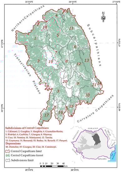
Figure 1.
The geographical study area of the Central Carpathians in Romania.
2.2. Forest Imagery and Pre-Processing
The analysis of deforestation patterns in Central Carpathians followed three main steps as shown in the flowchart (Figure 2). The first is related to the Landsat-7 Enhanced Thematic Mapper Plus (Landsat-7 ETM+) image data pre-processing and Geographic Information System Analysis (GIS analysis) for mapping the changes in deforestation patterns (Table 1), while the second part is the statistical validation (classification accuracy assessment) of them. The last part was based on the GLCM and fractal analysis of forest area dynamics.

Figure 2.
Flowchart of image data pre-processing and Geographic Information System Analysis (GIS analysis), accuracy assessment and Gray-Level Co-occurrence Matrix (GLCM) and fractal analysis of forest dynamics in Central Carpathians Romania.

Table 1.
Landsat-7 Enhanced Thematic Mapper Plus (Landsat-7 ETM+) image paths and rows covering the study area [42].
The process starts with the collection of satellite images from 2000–2017 (a spatial resolution of 30 m) from Global Forest Change (GFC) dataset from the Department of Geographical Sciences, University of Maryland (UMD) [41]. These images were used to extract the deforested areas (annually 2001 to 2017) and, tree cover areas.
The primary data source for our study is the GFC, and the process for obtaining the numerical information followed an entire algorithm.
The first step consisted of downloading the Raster data. Having a different projection (World Geodetic System (WGS) 84-European Petroleum Standards Group (EPSG): 4326) than the other spatial data (Dealul Piscului 1970 (Stereo 70)–European Petroleum Standards Group (EPSG): 31700), used in the study, a projection transformation step followed.
Next, a mask was applied to delineate the study area. To extract the numerical information, the raster image was converted from raster to vector, each pixel being transformed into a point by classes, but keeping all their properties. So, 18 classes were obtained for the deforestation image (class 0—was ignored because it corresponded to the entire surface of the study area—no interesting information, class 1 for deforestation of the year 2001, class 2 for deforestation of the year 2002, till class 17 for deforestation of 2017). From the tree cover image, of the same data source, 100 classes were obtained, each class corresponding to the degree of forest cover in each pixel (class 0 for pixels with 0% tree cover, class 100 to 100% tree cover). In all cases, the spatial dimension (resolution) of each pixel was taken by each point. For the numerical data extracted from the deforestation image, the number of the points for each class was multiplied with the surface of the point/spatial resolution of pixel (24.514 × 24.514 = 600.97 m²), but for the tree cover, the entire surface (600.97 m²) was giving only for pixels/points in class 100 (with 100% of tree cover). For the other classes, the surface decreasing proportionally, until class 0.
In order to have accurate information, and to compare with other economic indicators at a territorial administrative unit level, a spatial join was done. Then, all this information was compiled into Excel tables, which were used to continue the analysis.
2.3. Classification Accuracy Assessment
The GFC dataset for Central Carpathians results for 2001–2017 has been compared to a Google Earth image (February 2017) classified into deforested and non-deforested for validation purposes. Two hundred random ground reference test points have been selected and analysed, and classification error matrices have been calculated to estimate the accuracy assessment of the obtained GFC dataset (Figure 3a–c). In the selection of ground reference test points, some bias in the classification result may arise. It turns out that the agreement between the GFC dataset and the Google Earth Image mappings is very high (see Table 2) with an overall classification accuracy of 97%. In the GFC dataset, 96% of non-deforested pixels where correctly classified (Producer’s Accuracy and User’s Accuracy = 98% and commission error = 2.5% and omission error = 1.54%), whereas for the deforested pixels, the Producer’s Accuracy = 60% and User’s Accuracy = 50%. The confusion between deforested and non-deforested pixels is easily explained due to ground control errors or preprocessing from the GFC dataset (i.e., some pixels are classified as deforested ones even though there are observed compact forests; also, the pastures with clumps of forest are classified as deforested areas).
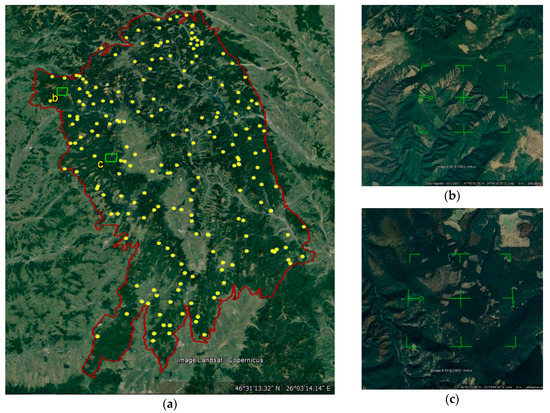
Figure 3.
(a) Random ground reference test points used for the accuracy assessment of Central Carpathians marked with yellow points; the two plots marked in light green square from the top (b) to the bottom (c) are representative plots with clear deforested areas; (b) Clear cuttings in Vatava TAU in Călimani Mountains; (c) Clear cuttings from 2017 in the Joseni TAU in Gurghiu Mountains.
Table 2.
Classification error matrix for Global Forest Change (GFC) dataset for Central Carpathians.
2.4. Preprocessing of GFC for GLCM and Fractal Analysis
To perform the GLCM and fractal analysis, it was necessary to go through several processes for making the maps for analysis. The first step was to estimate the tree cover and loss areas for Central Carpathians in grayscale. The second requirement was to export images to the same proportional scale in TIFF format to preserve their properties.
Subsequently, images were transformed into binary images using ImageJ 1.52 [43] and analysed using a macro for calculating the area and the percentage of forest pixels. The binarization was made by converting foreground pixels (which in turn corresponds to tree cover and loss) of grey and white tones, with intensities between 1 and 255, only in white pixels with the intensity of 255. The black background pixels (non-tree cover and non-loss) with 0 intensity remained the same.
The resolution of the analyzed images was 2716 × 2716 pixels. Pixels representing the tree cover and loss areas are automatically extracted from the GFC dataset on a grey scale. These images were used for Entropy GLCM analysis, but for the and FFI, the same images were binarized, all pixels indicating tree cover and loss becoming white.
GFC dataset provides information about the 2000 tree cover and loss areas for 2001–2017. Using the function Image Calculator operator (from ImageJ) the cumulative loss and tree cover data were obtained. Cumulative loss (the summed values for each year) was obtained using the Add function in Image Calculator. i.e., Cumulative loss for 2017 was obtained by adding the loss of each year from 2001 to 2017. The tree cover for the years 2001–2017 was obtained by using the Difference function in the Image Calculator. i.e., Tree cover 2017 was obtained by using difference between Tree cover 2000 and Cumulative loss 2017.
2.5. GLCM and Fractal Analysis
GLCM analysis, also known as the grey-level spatial dependence matrix, is a statistical method of examining texture that considers the spatial relationship of pixels. The GLCM functions characterise the composition of an image by calculating how often pairs of the pixel of specific values and in a specified spatial relationship occur in an image, creating a GLCM, and then extracting statistical measures from this matrix. They provide information about shape, i.e., the spatial relationships of pixels in an image. The GLCM measures how often a pixel of grey-level 8-bits images (grayscale intensity or tone) value i occurs either horizontally, vertically, or diagonally to adjacent pixels with the value j.
To determine the Entropy, a significant method for non-texturally uniform images and for small values of elements, a GLCM analysis was used.
Complex textures tend to have high entropy values. The entropy is measured according to Equation (1) [44].
where p(i,j) are co-occurrence probabilities and i and j are coordinates of the co-occurrence matrix.
Entropy measures the degree of disorder inside patches of tree cover and loss based on the relationship between pixels with different degrees of forest coverage. Complex texture tends to have high entropy values. The entropy expresses the degree of disturbance of the tree cover canopy of the forest, and it is in strong relation with the degree of fragmentation expressed by FFI. GLCM Entropy is complemented by FFI and , two binary analyzes, where all foreground pixels become white, measure the degree of fragmentation of the patches, some relative to each other.
For the analysis of fractal indices as FFI and , were used FFI plugin [45] and Frac2D plugin [46] in the IQM 3.5 software [47].
These indices are relevant because they quantify the spatial pattern of tree cover and loss areas by analysing the degree of fragmentation (FFI), and heterogeneity (). It is expected that as the loss increases, fragmentation and heterogeneity of forests will increase and at the same time a process of homogenization and compacting of cumulative losses will occur.
Fractal fragmentation is very useful in estimating fragmentation or compaction of fractal and natural objects that do not follow the classical geometry. FFI is calculated according to the Equation (2) and can be interpreted as a compaction index [40]:
where is the box-counting fractal dimension of the summed-up areas; is the box-counting fractal dimension of the summed-up perimeters; ε is the side length of the box; N(ε) is the number of contiguous and non-overlapping boxes required to cover the area of the object; and N’(ε) is the number of contiguous and non-overlapping boxes required to cover just the perimeter of the object [48,49].
The tree cover patches and loss are very small and highly fragmented and appear as point-like objects in the image; the degree of fragmentation is maximum, FFI = 0, according to Equation (2), in the situation where = . As the analyzed areas are more compact, the FFI value will increase to 1, and as they are more fragmented, irregular, the FFI will be closer to 0. The maximum compaction, when the areas are perfectly geometric, have an FFI = 1. However, self-similar objects, such as forests, with an identical fractal dimension may differ significantly in their textural appearance [50,51]. Therefore, the use of fractal fragmentation only is not useful for discriminating against objects, while the fractal fragmentation dimension quantifies the way space is occupied, and the lacunarity completes the fractal dimension with its ability to quantify how space is filled. Moreover, lacunarity discriminates the spatial distribution of gaps in texture at multiple scales, and is not sensitive to the edges of the images. In this paper, the Tug-of-War algorithm lacunarity [46] was calculated based on the equation:
with is the number of boxes, is the second moment for each width as the median of values, each is the mean of squares of the counter values. and are two random variables for each width that indicate the accuracy and confidence.
Finally, , where p(r,i) is the number of occupied sites in the i-th box. The values are directly influenced by the heterogeneity of the spatial distribution of tree cover and loss areas. So, the indicates the size of deforestation when gaps are more unevenly distributed.
2.6. Validation of GLCM and Fractal Analysis Indices
To check the normality of the fractal and non-fractal indicators used in the present study, a Shapiro-Wilk statistical test has been applied, instead of the graphical one, due to the small amount of data (2001–2017). In such cases, this statistical test is more easily understood instead of graphical ones. The data displayed in Table 3 indicate a normal distribution (W values—over 0.75). This hypothesis is also sustained by the p-values, which are above 0.05 in most cases. The p-values close to 0.05 are in direct accordance with the degree of compactness of tree cover or deforested areas.
Table 3.
Shapiro-Wilk test for the validation of data.
3. Results
3.1. The Analysis of Deforested Areas from Central Carpathians
In the Central Carpathians, the general decrease of the forest areas during 2000–2017 was observed, however with considerable inter-annual variability. Forest areas have continuously decreased during the period of analysis covering 967.646 ha in 2000 and 870.574 ha in 2017, but with some inter-annual variability. The highest average annual decreases are characterised 2007 and 2012, and the lowest values were observed in 2003 and 2013–2015. In total, 100.613 ha was deforested during the entire period of analysis, corresponding to a reduction in forest area by 11%. (Figure 4).

Figure 4.
Deforestation in Central Carpathians. The red patches mark the deforested areas meanwhile with green mark the forest areas.
In Figure 5a, the central aspect relates to the fact that the tree cover areas are diminishing, and the deforested areas are increasing with some annual variabilities. Also, the highest values of deforested areas were observed in 2007 (14.003 ha.) and 2012 (9.325 ha.).
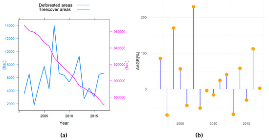
Figure 5.
(a) Dynamics of tree cover and deforested areas and in the Central Carpathians: the primary y-axis corresponds to the deforested areas in left part and tree cover areas in right part; (b) plot representing the Annual Average Growth Deforestation (AAGDR).
An important aspect is related to the Annual Average Growth Deforestation Rate (AAGDR) (Figure 5b) that was calculated according to the formula:
The AAGDR values present the high rate of growth of deforestation because the deforested areas are reduced from year to year, mainly in 2007 (229.14%) and in 2016 (112.25%) Until 2004, the deforestation is shown to be dispersed in small patches, but from 2005 and onwards clustering of deforestation can be observed. This aspect coincides with an overall diminishing of clusters for the tree cover areas.
3.2. Correlation between Deforested Areas and Logging Activities
An important disturbance agent of forest dynamics is represented by the logging activities that are in strong relation with the high deforestation rates. To have a more quantitative causal link between these two components, we have correlated the indicators of economic activities from the Classification of the Activities from the National Economy (NACE code 0220-logging activities) with the deforestation rates, registered at each Territorial Administrative Unit, from Central Carpathians. Figure 6 (a–d) show that for all the four economic indicators, the deforestation rates have no relation with the dimension of logging activities, being distributed on both the two axes. Many territorial administrative units have low concentrations of companies and employees, and low values of profit and turnover with small logging activities. Only some separate territorial administrative-units appear with high values for the four economic indicators. It is those ones where the palette of the economic activities is reduced to forestry activities (the monospecialized ones, from the economic point of view).
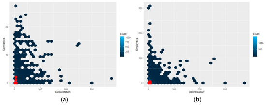
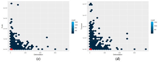
Figure 6.
Hexbin plot revealing a 2-dimension spatial distribution of (a) number of companies; (b) number of employees; (c) values of profit; (d) values of turnover, where the color-scheme defines the abundance of values.
3.3. The Analysis of GLCM Entropy
The Entropy of tree cover areas was relatively high and steadily increasing from 2.40 in 2000 to 2.51 in 2017 (change of 0.11). The main reason is a very different type of deforestation practices. However, the entropy values of the deforested areas were relatively small and constant over the period 2000–2014. Only two slight peaks (> 0.03) occurred in 2007 (0.05) and 2012 (0.04) coinciding with the highest deforestation rates. The lowest values of entropy (≤ 0.01) coincide with the lowest deforestation rates, which occurred in 2003 and 2013–2015 (Figure 7a).
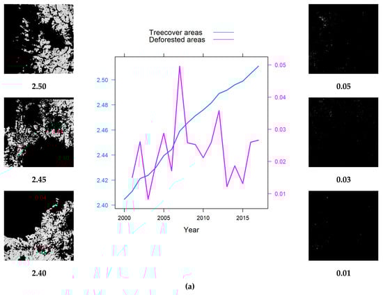
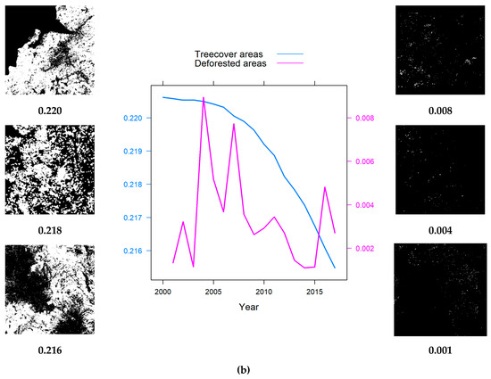
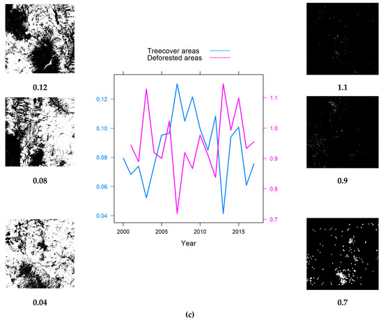
Figure 7.
(a) The GLCM Entropy dynamics induced by the computer-generated patterns-tree cover (left) and deforested areas (right)-as a function of their values. (b) The FFI dynamics induced by the computer-generated patterns—tree cover (left) and deforested areas (right)—as a function of their values. (c) The ΛT-o-W dynamics induced by the computer-generated patterns—tree cover (left) and deforested areas (right)—as a function of their values.
3.4. The Analysed Fractal Indices
The fractal indicators examined were FFI and The FFI values were reduced from 0.22 (2000) to 0.21 (2017) indicating a continuous growth of fragmentation of tree cover areas, with a reduction or even elimination of clusters of tree cover areas. The decrease of FFI, which indicates the increase in fractal fragmentation, is generated by the fragmentation of the patches, and the increase in their number by the detachment of the compact surfaces following the deforestation.
The fragmentation of the deforestation during 2001–2007 was very low; the FFI values between 0.001 (2001) and 0.008 (2007). Slightly more compacted deforestation with values > 0.003 occurred in 2004 and 2007, while fragmented deforestations with values < 0.001 were recorded in 2001, 2003 and 2013–2015 (Figure 7b). The degree of heterogeneity of tree cover areas was calculated using which highlighted the effects of deforestation on the compactness of tree cover areas. The lacunarity of tree cover areas decreased from 0.08 in 2000 to 0.011 in 2014 due to inter-annual variability of deforestation. An accentuated clustering of the deforestation (low values of ) corresponded with homogenous and compacted deforestations (lowest in 2004 and 2011) in comparison to years with more heterogeneous and fragmented deforestations in 2003 and 2013 (Figure 7c).
The most heterogeneous manifestation of deforestation (> 1) occurred in 2003, 2006 and 2013–2015. The most homogenous deforestations in a more compact manner with ≤ 0.8 were in 2007 and 2012.
4. Discussion
4.1. Deforestation changes in Central Carpathians
Results indicated an increase in deforested areas Central Carpathians from Romania during recent decades. By using satellite images from GFC, the information describing the situation of tree cover and deforested areas from a subdivision of Romanian Carpathians during the period 2000–2017 is provided. The satellite analysis of tree cover and deforested areas was complemented by GLCM and fractal analysis describing differentiations of forest disturbance, providing a quantification of changes in the heterogeneity and fragmentation of forest areas.
A general increment trend characterizes deforested areas in Romanian Carpathians due to high rates of illegal logging [8]. The significant changes in forestry legislation reveal that this growth in deforested areas resulted from the restitution of forest to former owners the Law 247/2005 [52] and privation of forests, especially in the mountain areas [8,10,34,53]. Among various natural and anthropic perturbations in forest areas from Central Carpathians, the logging activities represent an important factor of disturbance, determining the growth of logging activities [54].
4.2. Use of GLCM and Fractal Analysis for Quantification the Deforestation Changes
We have evaluated the forest and deforested areas [41] using the GLCM and fractal analysis, determining the entropy with FFI and ΛT-o-W. This research demonstrates the usefulness of GLCM and fractal analysis for the measurement of deforestation patterns [55]. The findings of this study confirmed the hypothesis that fractal analysis adds interesting ways of measuring the degree of fragmentation of tree cover areas caused by the deforestation. Here, GLCM and fractal analysis are used to study the characteristic of deforested and tree cover areas in Central Carpathians.
In the GLCM analysis of tree cover and deforested areas, the entropy analysis is used to describe the spatial relationship between pixels [56]. For the fractal analysis, the FFI and ΛT-o-W methods were performed to define the degree of fragmentation of tree cover areas determined by forest disturbances. In previous studies, fractal analysis of tree cover and deforested areas were calculated by using the FFI [40,57,58], Fixed Grid 2D Lacunarity (FG2DL) [59]. Until now, fractal analysis was used in urban agglomeration, urban growth [60,61,62], or green infrastructure models of cities [63].
The main findings are discussed in the following aspects:
- Fractal methods may provide valuable complementary information to currently available methodologies in the field of forestry research;
- A continuous decrease of tree cover areas has occurred during the period of analysis, however with considerable inter-annual variability;
- Results indicate that, as the loss areas increased, forest fragmentation and heterogeneity also increased. The process of homogenization and compaction of cumulative loss has also been confirmed;
- Differences between the fractal and GLCM indices arise from the type of image analyzed and from the information extracted. For the Entropy, the images are grey-scale 8-bits, and we obtain the clutter of spatial pixel distribution in grayscale within patches of tree cover and loss. Thus, the analysis is at the level of forest cover as the forest looks dense. For and FFI, the images are binary, and we extract information about how these patches are spatially distributed, regardless of how the forest looks or how loss has occurred within these patches, resulting in anti-parallel developments.
Spatial patterns changes can be distinguished between the analysis of deforested and tree cover areas. The period with more intense deforestation is characterized by a more compact and homogenous way, but disordered at the level of patch forest cover, and vice versa. As the deforestation increases, the cumulative deforested areas increase gradually, with a decrease in the heterogeneity of spatial distribution of the deforested patches and an increase in tree cover disorder around them. The newly deforested areas are made as new patches, alternating with agglutinations around patches previously deforested. Regarding the spatial patterns of tree cover areas, as the deforested areas increase, there is a tendency to increase fractal fragmentation of forests; this is associated with an increase in patch-level forest clutter. of tree cover shows tight yearly oscillations related to the degree of heterogeneity of deforested areas.
4.3. Prospects About Sustainable Forest Management
The current paper explains the importance of using the entropy, FFI and for the better understanding of tree cover areas and its immediate effects as deforestation. The method, based on GLCM and fractal analysis, exemplifies the advantage of making known the effects of forest fragmentation. The fragmentation affects the stability of forest ecosystems and determines the decrease of biodiversity and rare species of fauna and flora [17,18]. The analysis of deforestation by fractal analysis provides complementary information to the already known methods of deforestation mapping.
5. Conclusions
Here, an analysis of Landsat-7 ETM+ satellite images at 30 m resolution in Central Carpathians is provided, offering quantitative information describing the spatial and temporal dynamics of deforestation and tree cover areas during the period of analysis (2000–2017). Based on the fractal analysis that can expertly analyse irregular spatial structures, new information about deforestation—as described by textural uniformity, compactness and chaotic distribution of the forest—disturbance processes were obtained. The analysis of fractal indicators (entropy, FFI and ) describes and quantifies the textural uniformity, compactness and chaotic distribution of the disturbance processes of deforestation. Overall, the Central Carpathians is a region with a highly deforested mountainous area. It is concluded that fractal analysis of deforested areas is an effective tool in quantifying the degree of homogeneity or spatial heterogeneity of deforested areas. Analysis of the degree of textural disorder of deforestation in tree cover areas provides essential information to identify efficient methods for managing legal as well as illegal logging. Such quantitative metrics can also assist in identifying the impact of forest disturbances on biodiversity and local economies and may act as guidance for policy makers from deforested territorial administrative units from Central Carpathians.
Author Contributions
Conceptualization, A.-M.C., I.A., R.-D.P. and D.P.; Data curation, R.-A.R. and A.G.; Formal analysis, I.A.; Funding acquisition, C.-C.D.; Investigation, C.-C.D., R.-M.P. and M.M.; Methodology, I.A., H.A. and M.R.; Project administration, A.K.G. and I.-V.L.; Resources, I.A., R.-D.P. and D.P.; Software, I.A., H.F.J., M.R. and A.-G.S.; Supervision, A.-M.C., I.A. and D.P.; Validation, I.A., H.A., D.P. and R.F.; Visualization, D.P.; Writing—Original draft, A.-M.C., R.-D.P. and R.F.; Writing—Review & editing, A.-M.C. and R.F.
Funding
This research received no external funding.
Acknowledgments
The authors want to thank Arshad Ali from Spatial Ecology Lab, School of Life Sciences, South China Normal University, China for his advice and great comments to improve the paper and our colleague Mircea Cristian Vișan for his help related to electronic mapping.
Conflicts of Interest
The authors declare no conflict of interest.
References
- Grebner, D.L.; Bettinger, P.; Siry, J.P. A Brief History of Forestry and Natural Resource Management. In Introduction to Forestry and Natural Resources; Academic Press: Waltham, MA, USA, 2013; pp. 1–20. [Google Scholar]
- Hossain, S.M.Y.; Robak, E.W. A Forest Management Process to Incorporate Multiple Objectives: A Framework for Systematic Public Input. Forests 2010, 1, 99–113. [Google Scholar] [CrossRef]
- Nordlund, A.; Westin, K. Forest Values and Forest Management Attitudes among Private Forest Owners in Sweden. Forests 2011, 2, 30–50. [Google Scholar] [CrossRef]
- Beaudoin, G.; Rafanoharana, S.; Boissiere, M.; Wijaya, A.; Wardhana, W. Completing the Picture: Importance of Considering Participatory Mapping for REDD plus Measurement, Reporting and Verification (MRV). PLoS ONE 2016, 11, e0166592. [Google Scholar] [CrossRef]
- Borrelli, P.; Panagos, P.; Marker, M.; Modugno, S.; Schütt, B. Assessment of the impacts of clear-cutting on soil loss by water erosion in Italian forests: First comprehensive monitoring and modelling approach. Catena 2017, 149, 770–781. [Google Scholar] [CrossRef]
- Pazur, R.; Bolliger, J. Land changes in Slovakia: Past processes and future directions. Appl. Geogr. 2017, 85, 163–175. [Google Scholar] [CrossRef]
- Bayer, A.D.; Lindeskog, M.; Pugh, T.A.M.; Anthoni, P.M.; Fuchs, R.; Arneth, A. Uncertainties in the land-use flux resulting from land-use change reconstructions and gross land transitions. Earth Syst. Dyn. 2017, 8, 91–111. [Google Scholar] [CrossRef]
- Knorn, J.; Kuemmerle, T.; Radeloff, V.C.; Szabo, A.; Mîndrescu, M.; Keeton, W.S.; Abrudan, I.; Griffiths, P.; Gancz, V.; Hostert, P. Forest restitution and protected area effectiveness in post-socialist Romania. Biol. Conserv. 2012, 146, 204–212. [Google Scholar] [CrossRef]
- Bouriaud, L.; Nichiforel, L.; Weiss, G.; Bajraktari, A.; Curovic, M.; Dobsinska, Z.; Glavonjic, P.; Jarsky, V.; Sarvasova, Z.; Teder, M.; et al. Governance of private forests in Eastern and Central Europe: An analysis of forest harvesting and management rights. Ann. For. Res. 2013, 56, 199–215. [Google Scholar]
- Crăciunescu, A.; Stanciu, S.; Moatăr, M. The Implementation of European Forest Legislation for a Sustainable Development. Res. J. Agric. Sci. 2014, 46, 158–165. [Google Scholar]
- Cojoc, G.M.; Romanescu, G.; Tirnovan, A. Exceptional floods on a developed river: Case study for the Bistrița River from the Eastern Carpathians (Romania). Nat. Hazards 2015, 77, 1421–1451. [Google Scholar] [CrossRef]
- Stoffel, M.; Wyzga, B.; Marston, R.A. Floods in mountain environments: A synthesis. Geomorphology 2016, 272, 1–9. [Google Scholar] [CrossRef]
- Simons, P. After Skiing, The Deluge—Deforestation Increases Avalanches and Landslides in The Alps. New Sci. 1988, 117, 49–52. [Google Scholar]
- Comănescu, L.; Nedelea, A. Public perception of the hazards affecting geomorphological heritage-case study: The central area of Bucegi Mts. (Southern Carpathians, Romania). Environ. Earth Sci. 2015, 73, 8487–8497. [Google Scholar] [CrossRef]
- Malek, Z.; Boerboom, L.; Glade, T. Future Forest Cover Change Scenarios with Implications for Landslide Risk: An Example from Buzău Subcarpathians, Romania. Environ. Manag. 2015, 56, 1228–1243. [Google Scholar] [CrossRef]
- De la Paix, M.J.; Lanhai, L.; Xi, C.; Ahmed, S.; Varenyam, A. Soil Degradation and Altered Flood Risk as a Consequence of Deforestation. Land Degrad. Dev. 2013, 24, 478–485. [Google Scholar] [CrossRef]
- Fahrig, L. Effects of habitat fragmentation on biodiversity. Annu. Rev. Ecol. Evol. Syst. 2003, 34, 487–515. [Google Scholar] [CrossRef]
- Gamfeldt, L.; Snall, T.; Bagchi, R.; Jonsson, M.; Gustafsson, L.; Kjellander, P.; Ruiz-Jaen, M.C.; Froberg, M.; Stendahl, J.; Philipson, C.D.; et al. Higher levels of multiple ecosystem services are found in forests with more tree species. Nat. Commun. 2013, 4, 1340. [Google Scholar] [CrossRef]
- Karstensen, J.; Peters, G.P.; Andrew, R.M. Attribution of CO2 emissions from Brazilian deforestation to consumers between 1990 and 2010. Environ. Res. Lett. 2013, 8, 2. [Google Scholar] [CrossRef]
- Kaplan, J.O.; Krumhardt, K.M.; Gaillard, M.J.; Sugita, S.; Trondman, A.K.; Fyfe, R.; Marquer, L.; Mazier, F.; Nielsen, A.B. Constraining the Deforestation History of Europe: Evaluation of Historical Land Use Scenarios with Pollen-Based Land Cover Reconstructions. Land 2017, 6, 4. [Google Scholar] [CrossRef]
- Krasovskii, A.; Khaharov, N.; Ohersteiner, M. CO2-intensive power generation and REDD-based emission offsets with a benefit-sharing mechanism. Energy Syst. 2017, 8, 857–883. [Google Scholar] [CrossRef]
- Chakravarty, S.; Ghosh, S.K.; Suresh, C.P.; Dey, A.N.; Shukla, G. Deforestation: Causes, Effects and Control Strategies. Global Perspectives on Sustainable Forest Management 2012. Available online: http://cdn.intechopen.com/pdfs/36125/InTechDeforestation_causes_effects_and_control_strategies.pdf (accessed on 24 February 2019).
- Food and Agriculture Organization of the United Nations—Deforestation. Available online: http://www.fao.org/3/j9345e/j9345e07.htm (accessed on 24 February 2019).
- Spiecker, H. Silvicultural management in maintaining biodiversity and resistance of forests in Europe-temperate zone. J. Environ. Manag. 2003, 67, 55–65. [Google Scholar] [CrossRef]
- Vitasse, Y.; Francois, C.; Delpierre, N.; Dufrene, E.; Kremer, A.; Chuine, I.; Delzon, S. Assessing the effects of climate change on the phenology of European temperate trees. Agric. For. Meteorol. 2011, 151, 969–980. [Google Scholar] [CrossRef]
- Domingo, F.; Puigdefabregas, J.; Moro, M.J.; Bellot, J. Role of Vegetation Cover in the Biogeochemical Balances of Small Afforested Catchment in Southeastern Spain. J. Hydrol. 1994, 159, 275–289. [Google Scholar] [CrossRef]
- Robinson, M.; Cognard-Plancq, A.L.; Cosandey, C.; David, J.; Durand, P.; Fuhrer, H.W.; Hall, R.; Hendriques, M.O.; Marc, V.; McCarthy, R.; et al. Studies of the impact of forests on peak flows and baseflows: A European perspective. For. Ecol. Manag. 2003, 186, 85–97. [Google Scholar] [CrossRef]
- Lim, S.S.; Innes, J.L.; Sheppard, S.R.J. Awareness of Aesthetic and Other Forest Values: The Role of Forestry Knowledge and Education. Soc. Nat. Resour. 2015, 28, 1308–1322. [Google Scholar] [CrossRef]
- Lim, S.S.; Innes, J.L. Forest aesthetic indicators in sustainable forest management standards. Can. J. For. Res. 2017, 47, 536–544. [Google Scholar] [CrossRef]
- Veen, P.; Fanta, J.; Raev, I.; Biris, I.A.; de Smidt, J.; Maes, B. Virgin forests in Romania and Bulgaria: Results of two national inventory projects and their implications for protection. Biodivers. Conserv. 2010, 19, 1805–1819. [Google Scholar] [CrossRef]
- Hurdu, B.I.; Pușcaș, M. Centres of endemism, spatial barriers and biogeography of the South-Eastern Carpathians inferred from multivariate analysis of endemic plant species distribution. Acta Biol. Ser. Bot. 2013, 55, 24. [Google Scholar]
- Price, M.F.; Gratzer, G.; Duguma, L.A.; Kohler, T.; Maselli, D.; Romeo, R. Mountain Forests in a Changing World—Realizing Values, Addressing Challenges; FAO/MPS and SDC: Rome, Italy, 2011; pp. 1–86. [Google Scholar]
- Mraz, P.; Ronikier, M. Biogeography of the Carpathians: Evolutionary and spatial facets of biodiversity. Biol. J. Linn. Soc. 2016, 119, 528–559. [Google Scholar] [CrossRef]
- Abrudan, I.V.; Marinescu, V.; Ionescu, O.; Ioras, F.; Horodnic, S.A.; Sestras, R. Developments in the Romanian Forestry and its linkages with other sectors. Not. Cluj-Napoca 2009, 37, 14–21. [Google Scholar]
- Banski, J. Changes in agricultural land ownership in Poland in the period of the market economy. Agric. Econ. Zemed. 2011, 57, 93–101. [Google Scholar]
- Sarvasova, Z.; Zivojinovic, I.; Weiss, G.; Dobsinska, Z.; Dragoi, M.; Gal, J.; Jarsky, V.; Mizaraite, D.; Pollumae, P.; Salka, J.; et al. Forest Owners Associations in the Central and Eastern European Region. Small-Scale For. 2015, 14, 217–232. [Google Scholar] [CrossRef]
- Kuemmerle, T.; Hostert, P.; Radeloff, V.C.; Perzanowski, K.; Kruhlov, I. Post-socialist forest disturbance in the Carpathian border region of Poland, Slovakia, and Ukraine. Ecol. Indic. 2007, 17, 1279–1295. [Google Scholar] [CrossRef]
- Griffiths, P.; Kuemmerle, T.; Baumann, M.; Radeloff, V.C.; Abrudan, I.V.; Lieskovsky, J.; Munteanu, C.; Ostapowicz, K.; Hostert, P. Forest disturbances, forest recovery, and changes in forest types across the Carpathian ecoregion from 1985 to 2010 based on Landsat image composites. Remote Sens. Environ. 2014, 151, 72–88. [Google Scholar] [CrossRef]
- Sun, J.; Huang, Z.J.; Zhen, Q.; Southworth, J.; Perz, S. Fractally deforested landscape: Pattern and process in a tri-national Amazon frontier. Appl. Geogr. 2014, 52, 204–211. [Google Scholar] [CrossRef]
- Andronache, I.; Ahammer, H.; Jelinek, H.F.; Peptenatu, D.; Ciobotaru, A.-M.; Drăghici, C.-C.; Pintilii, R.D.; Simion, A.G.; Teodorescu, C. Fractal analysis for studying the evolution of forests. Chaossolitons Fractals 2016, 91, 310–318. [Google Scholar] [CrossRef]
- Hansen, M.C.; Potapov, P.V.; Moore, R.; Hancher, M.; Turubanova, S.A.; Tyukavina, A.; Thau, D.; Stehman, S.V.; Goetz, S.J.; Loveland, T.R.; et al. High-Resolution Global Maps of 21st-Century Forest Cover Change. Science 2013, 342, 850–853. Available online: http://earthenginepartners.appspot.com/science-2013-global-forest (accessed on 21 January 2016). [CrossRef] [PubMed]
- Andronache, I.; Fensholt, R.; Ahammer, H.; Ciobotaru, A.-M.; Pintilii, R.-D.; Peptenatu, D.; Drăghici, C.-C.; Diaconu, D.C.; Radulovic, M.; Pulighe, G.; et al. Assessment of Textural Differentiations in Forest Resources in Romania Using Fractal Analysis. Forests 2017, 8, 54. [Google Scholar] [CrossRef]
- Schneider, C.A.; Rasband, W.S.; Eliceiri, K.W. NIH Image to ImageJ: 25 years of image analysis. Nat. Methods 2012, 9, 671–675. [Google Scholar] [CrossRef]
- Haralick, R.M.; Shanmugam, K.; Dinstein, I. Texture parameters for image classification. IEEE Trans. Syst. Man Cybern. 1973, SMC-3, 610–621. [Google Scholar] [CrossRef]
- Ahammer, H.; Andronache, I. IQM Plugin FFI. 2016. Available online: https://sourceforge.net/projects/iqm-plugin-ffi/ (accessed on 6 January 2017).
- Reiss, M.A.; Lemmerer, B.; Hanslmeier, A.; Ahammer, H. Tug-of-war lacunarity—A novel approach for estimating lacunarity. Chaos 2016, 26, 113102. [Google Scholar] [CrossRef] [PubMed]
- Kainz, P.; Mayrhofer-Reinhartshuber, M.; Ahammer, H. IQM: An Extensible and Portable Open Source Application for Image and Signal Analysis in Java. PLoS ONE 2015, 10, e0116329. [Google Scholar] [CrossRef]
- Russel, D.; Hanson, J.; Ott, E. Dimension of strange attractors. Phys. Rev. Lett. 1980, 45, 1175–1178. [Google Scholar] [CrossRef]
- Karperien, A.; Ahammer, H.; Jelinek, H.F. Quantitating the subtleties of microglial morphology with fractal analysis. Front. Cell. Neurosci. 2013, 7. [Google Scholar] [CrossRef]
- Plotnick, R.E.; Gardner, R.H.; Oneill, R.V. Lacunarity Indexes as Measures of Landscape Texture. Landsc. Ecol. 1993, 8, 201–211. [Google Scholar] [CrossRef]
- Taylor, R.P.; Martin, T.P.; Montgomery, R.D.; Smith, J.H.; Micolich, A.P.; Boydston, C.; Scannell, B.C.; Fairbanks, M.S.; Spehar, B. Seeing shapes in seemingly random spatial patterns: Fractal analysis of Rorschach inkblots. PLoS ONE 2017, 12. [Google Scholar] [CrossRef]
- Romanian Government Official Monitor. Law no. 247/2005 on the Reform of Property and Justice, as Well as Some Accompanying Measures (Legea nr. 247 din 2005 Privind Reforma în Domeniile Proprietăţii şi Justiţiei, Precum şi unele Măsuri Adiacente). Available online: http://legislatie.just.ro/Public/DetaliiDocument/63447 (accessed on 24 February 2019).
- Munteanu, C.; Kuemmerle, T.; Keuler, N.S.; Muller, D.; Balazs, P.; Dobosz, M.; Griffiths, P.; Halada, L.; Kaim, D.; Kiraly, G.; et al. Legacies of 19th century land use shape contemporary forest cover. Glob. Environ. Chang. Hum. Policy Dimens. 2015, 34, 83–94. [Google Scholar] [CrossRef]
- Knorn, J.; Kuemmerle, T.; Radeloff, V.C.; Keeton, W.S.; Gancz, V.; Biris, I.A.; Svoboda, M.; Griffiths, P.; Hagatis, A.; Hostert, P. Continued loss of temperate old-growth forests in the Romanian Carpathians despite an increasing protected area network. Environ. Conserv. 2013, 40, 182–193. [Google Scholar] [CrossRef]
- Singh, M.; Evans, D.; Friess, D.A.; Tan, B.S.; Nin, C.S. Mapping Above-Ground Biomass in a Tropical Forest in Cambodia Using Canopy Textures Derived from Google Earth. Remote Sens. 2015, 7, 5057–5076. [Google Scholar] [CrossRef]
- Weissgerber, F.; Colin-Koeniguer, E.; Nicolas, N.; Nicolas, J.M. A Temporal Estimation of Entropy and Its Comparison With Spatial Estimations on PolSAR Images. IEEE J. Sel. Top. Appl. Earth Obs. Remote Sens. 2016, 9, 3809–3820. [Google Scholar] [CrossRef]
- Garcia-Gigorro, S.; Saura, S. Forest Fragmentation Estimated from Remotely Sensed Data: Is Comparison Across Scales Possible? For. Sci. 2005, 51, 51–63. [Google Scholar]
- Garcia, D.; Quevedo, M.; Obeso, J.R.; Abajo, A. Fragmentation patterns and protection of montane forest in the Cantabrian range (NW Spain). For. Ecol. Manag. 2005, 208, 29–43. [Google Scholar] [CrossRef]
- Pintilii, R.-D.; Andronache, I.; Diaconu, D.C.; Dobrea, R.C.; Zeleňáková, M.; Fensholt, R.; Peptenatu, D.; Drăghici, C.-C.; Ciobotaru, A.-M. Using Fractal Analysis in Modeling the Dynamics of Forest Areas and Economic Impact Assessment: Maramureș County, Romania, as a Case Study. Forests 2017, 8, 25. [Google Scholar] [CrossRef]
- Frankhauser, P. The fractal approach. A new tool for the spatial analysis of urban agglomerations. Population 1998, 10, 205–240. [Google Scholar]
- Tannier, C.; Pumain, D. Fractals in urban geography: A theoretical outline and an empirical example. Cybergeo Eur. J. Geogr. 2005, 307, 10–4000. [Google Scholar] [CrossRef]
- Chen, Y.G.; Feng, J. Spatial analysis of cities using Renyi entropy and fractal parameters. Chaos Solitons Fractals 2017, 105, 279–287. [Google Scholar] [CrossRef]
- Petrișor, A.I.; Andronache, I.; Petrișor, L.E.; Ciobotaru, A.M.; Peptenatu, D. Assessing the fragmentation of the green infrastructure in Romanian cities using fractal models and numerical taxonomy. Procedia Environ. Sci. 2016, 32, 110–123. [Google Scholar] [CrossRef]
© 2019 by the authors. Licensee MDPI, Basel, Switzerland. This article is an open access article distributed under the terms and conditions of the Creative Commons Attribution (CC BY) license (http://creativecommons.org/licenses/by/4.0/).