Article

Forest Site and Type Variability in ALS-Based Forest Resource Inventory Attribute Predictions over Three Ontario Forest Sites

1
Department of Geography and Planning, Queen’s University, Kingston, ON K7L 3N6, Canada
2
Forest Resource Inventory Unit, Ontario Ministry of Natural Resources, North Bay, ON P1A 4L7, Canada
3
Natural Resources Canada, Canadian Wood Fibre Centre, Canadian Forest Service, Sault Ste. Marie, ON P6A 2E5, Canada
4
Ontario Ministry of Natural Resources and Forestry, Science and Research Branch, 1235 Queen Street E, Sault Ste. Marie, ON P6A 2E5, Canada
5
Faculty of Forestry, University of Toronto, Toronto, ON M5S 3B3, Canada
*
Author to whom correspondence should be addressed.
Forests 2019, 10(3), 226; https://doi.org/10.3390/f10030226
Submission received: 21 December 2018 / Revised: 16 January 2019 / Accepted: 26 February 2019 / Published: 4 March 2019
(This article belongs to the Section Forest Inventory, Modeling and Remote Sensing)

Abstract

:
Over the last decade, spatially-explicit modeling of landscape-scale forest attributes for forest inventories has greatly benefitted from airborne laser scanning (ALS) and the area-based approach (ABA) to derive wall-to-wall maps of these forest attributes. Which ALS-derived metrics to include when modeling forest inventory attributes, and how prediction accuracies vary over forest types depends largely on the structural complexity of the forest(s) being studied. Hence, the purpose of this study was to (i) examine the usefulness of adding texture and intensity metrics to height-based ALS metrics for the prediction of several forest resource inventory (FRI) attributes in one boreal and two Great Lakes, St. Lawrence (GLSL) forest region sites in Ontario and (ii) quantify and compare the site and forest type variability within the context of the FRI prediction accuracies. Basal area (BA), quadratic mean diameter-at-breast height (QMD), and stem density (S) were predicted using the ABA and a nonparametric Random Forests (RF) regression model. At the site level, prediction accuracies (i.e., expressed as RMSE (Root Mean Square Error), bias, and R2) improved at the three sites when texture and intensity metrics were included in the predictor set, even though no significant differences (p > 0.05) could be detected using the nonparametric RMANOVA test. Stem density benefitted the most from the inclusion of texture and intensity, particularly in the GLSL sites (% RMSE improved up to 6%). Combining site and forest type results indicated that improvements in site level predictions, due to the addition of texture and intensity metrics to the ALS predictor set, were the result of changes in prediction accuracy in some but not all forest types present at a site and that these changes in prediction accuracy were site and FRI attribute specific. The nonparametric Kruskal–Wallis test indicated that prediction errors between the different forest types were significantly different (p ≤ 0.01). In the boreal site, prediction accuracies for conifer forest types were higher than for deciduous and mixedwoods. Such patterns in prediction accuracy among forest types and FRI attributes could not be observed in the GLSL sites. In the Petawawa Research Forest (PRF), we did detect the impact of silvicultural treatments especially on QMD and S predictions.

1. Introduction

Over the last decade, spatially-explicit modeling of landscape-scale forest attributes for forest inventories has greatly benefitted from airborne laser scanning (ALS), either as the only data source to model forest inventory attributes [1,2,3], in combination with multi- or hyperspectral imagery [4], or in combination with digital aerial photogrammetry (DAP) to update forest inventories [5] (for an overview see Wulder et al. [6]). ALS has shown great utility for capturing the three-dimensional structure of forest canopies [7] with ALS metrics, such as mean height of ALS returns, serving as suitable predictors of forest structural attributes. In the context of forest resource inventories (FRI), attributes such as timber volume (VOL), aboveground biomass (AGB), basal area (BA), quadratic mean diameter-at-breast height (QMD), and stem density (S) have been successfully estimated using ALS metrics, especially with area-based approaches (ABA), in a variety of forest ecosystems worldwide (e.g., [2,3,8,9,10,11,12,13,14]). These attributes are crucial for the assessment of carbon and growing stock, size-class distributions and timber assortment, and sustainable forest management (SFM) at local, provincial, national, and global scales.
Many studies have focused on what ALS metrics to include in the predictor set to improve FRI attribute predictions. Furthermore, an increasing number of studies are focusing on testing the generality and transferability of ALS-based predictions of FRI attributes over larger landscapes and for different forest sites to determine if relationships between key ALS metrics and FRI attributes remain consistent over multiple sites and multiple forest cover conditions [1,3,8,11,15,16,17]. Kotivuori et al. [17] found that forest structure and the specific ALS sensor and acquisition parameters have considerable effect on FRI attribute predictions when they compared nationwide to regional-level prediction models. The identification of key ALS metrics for the prediction of FRI attributes is important because over time, a large set of ALS metrics have been developed from normalized height (z) information contained in the ALS data. Given this plethora of ALS metrics, various authors have identified points of concern (e.g., [16,18,19]). For example, strong intercorrelations between metrics can cause problems in feature selection, i.e., the selection of a subset of predictors for a parsimonious and robust model, and model generalization for sites with different vegetation and terrain conditions [18,19,20]. They can also hamper the interpretation of the relationships between ALS metrics and predicted FRI variables [21]. Large numbers of highly correlated and redundant metrics can increase the likelihood that the selected predictors are sensitive to stochastic “noise” rather than general trends in the data [22]. This, in turn, may adversely affect model generalization, i.e., the quality of the predictions may decrease when applied to new data [23,24]. Based on reviews of the literature, White et al. [25,26] conclude that ALS metrics related to height, the variability of height, and canopy cover/density are often the most reliable predictors of FRI attributes. Others, e.g., Bouvier et al. [16], have argued that ALS metrics used for the prediction of FRI attributes should also incorporate ALS metrics that characterize the vertical structure of forest stands. Even though in most studies these ALS metrics explain the majority of variation within FRI attributes, additional ALS metrics may be required to improve FRI attribute predictions in more complex forest ecosystems, e.g., forest ecosystems with a large variety of tree species or ones undergoing partial-harvest silviculture, or when modeling more complex forest stand attributes such as diameter distributions.
Based on the utility of texture metrics derived from optical imagery for forestry applications (e.g., [27,28]), texture metrics have also been developed from ALS-based canopy height models (CHM) [29,30,31,32]. These texture metrics allow for a more detailed characterization of horizontal forest structure or upper canopy variability, i.e., in the prediction of species [29], growing stock attributes [31,33], and the spatial arrangement of trees [30,32]. Ozdemir and Donoghue [31] showed that texture metrics generated from ALS-derived canopy height models (CHM) explained tree size diversity (tree height and QMD diversity). Niemi and Vauhkonen [33] found that texture metrics improved predictions of VOL and BA in Finland’s boreal forest and helped cluster forest stands into groups with increasing maturity and stocking characteristics. Hence, texture appears to capture upper canopy variability which can be indicative of stand development stage [33].
Intensity metrics are another set of ALS metrics that, until recently, have generally been excluded from ALS metric sets for the prediction of FRI attributes because of the radiometric heterogeneities in uncalibrated intensity values due to system- and environment-induced distortions [34]. These distortions degrade the intensity quality and hence may reduce the performance and robustness of the predictive models applied. However, some studies have incorporated intensity-based ALS metrics to improve ABA growing stock [35], diameter distribution models [36], tree species classification [37], and gap fraction [38]. The utility of intensity data is primarily attributed to its ability to discriminate among tree species and characterize foliage distribution within the canopy [39]. Shang et al. [36] postulated that intensity metrics may capture the permeability or layering of the canopy. For example, early forest stand development stages are characterized by simple forest structure which results in a relatively low overall canopy density/high canopy permeability. In such stands the authors observed low variance of intensity values.
The variability in FRI attribute prediction accuracy within forest types has been addressed either by predicting FRI attributes separately by forest type [9,10,13,40,41,42,43,44,45] or by predicting FRI attributes over the entire forest site and subsequently extracting predictions (and error) by forest type (e.g. [13,44,45]). For example, Pitt et al. [44] found that the quality of FRI attribute predictions varied with forest type regardless of which prediction method used. Studies in boreal and temperate regions in Europe (e.g., [40,41,43,46]) found more accurate predictions of FRI attribute estimates for conifers than deciduous or mixed forest types. However, Spriggs et al. [45] found that BA and S were more accurately predicted for broadleaved species than conifers in the Great Lakes, St. Lawrence (GLSL) forest region in Ontario. The authors postulated that estimation models fit dominant forest type better. Hence, prediction accuracies for coniferous species are better in boreal regions (where conifers are dominant), whereas prediction accuracies for deciduous species are better in deciduous dominated forests such as the GLSL. In addition, Heurich and Thoma [42] found that not only forest species composition but also forest management practices influenced the relationships between FRI attribute prediction accuracies and the ALS-based predictors. Their FRI prediction accuracies showed no significant differences between deciduous and coniferous forest areas in a montane mixed forest in Germany which they attributed to selective harvesting activities within some of the conifer stands and that subsequently lowered the overall predictive accuracies in their conifer forest area.
Here, we examine the inclusion of CHM texture and intensity metrics on FRI attribute prediction of BA, QMD, and S because these metrics characterize stand structural properties not characterized by ALS metrics derived from the normalized height information. We test these metrics at three study sites in Ontario that vary in terms of forest complexity. We then compare forest site and forest type variability in the FRI attribute prediction accuracies within and between these sites to determine how FRI predictions and errors vary. We ask the following questions.
(1)
How does the inclusion of CHM texture and/or intensity information affect the FRI attribute prediction accuracy at the overall site level? We hypothesize that the addition of texture and intensity information will benefit predictions more for complex forest ecosystems, i.e., the GLSL, than for structurally simpler forest ecosystems, i.e., the boreal forest region.
(2)
How does inclusion of CHM texture and/or and intensity information affect FRI attribute prediction accuracy at the forest type level? Are FRI attribute prediction errors within forest types significantly different from each other within and between sites and how does it change when additional texture and/or intensity metrics are used in the predictions.

2. Materials and Methods

2.1. Study Sites

We conducted our research across three forest sites in northern and central Ontario, Canada to capture some of the diversity that exists within Ontario’s managed forest ecosystems (Figure 1). One forest site is representative of the boreal forest region (i.e., Hearst Forest (HF)) and two sites represent the GLSL forest region (i.e., Petawawa Research Forest (PRF) and Haliburton Forest and Wildlife Reserve (HFWR)), the transitional zone between the northern boreal forest and the eastern deciduous forest of North America. Even though PRF and HFWR are both in the GLSL forest region, they do differ in terms of species composition. Due to differences in annual precipitation, soils, and management practices, PRF tends to be dominated by conifer species while HFWR is more hardwood dominated. For forest management planning purposes, Ontario recognizes eight provincial forest types that have been grouped by ecological and site characteristics such as species composition and ecosite: (i) white and red pine (white and red pine mixedwood stands); (ii) jack pine; (iii) upland conifers (predominantly mixed spruce, jack pine, and fir stands on upland sites); (iv) lowland conifers (predominantly black spruce stands on low, poorly drained sites); (v) mixedwood (mixed stands containing spruce, jack pine, fir, poplar, and white birch); (vi) poplar; (vii) white birch; and (viii) tolerant hardwoods (predominantly maple and oak). Variability does exist within these forest types, e.g., mixedwoods and tolerant hardwoods are more heterogeneous than jack pine. This can be attributed to varying stand development and seral stages, stand age, understory species composition, natural disturbances, and the impact of silvicultural practices. The three study sites overlap in provincial forest types to some extent, i.e., forested wetlands (lowland conifers), spruce forests (upland conifers), intolerant hardwoods (poplar and white birch), and mixedwoods stands can be found at all three sites. However, these forest types and sites are managed differently, i.e., spruce forests are managed at HF and unmanaged at HFWR. Tolerant hardwoods are only found in the GLSL forest region sites and the pine forest types are only encountered at HF and PRF.

2.1.1. Hearst Forest (HF)

The Hearst Forest (49°40′ N, 83°40′ W) is located in northeastern Ontario and is the largest of the three sites (1,200,000 hectares) of which more than 1,000,000 ha is productive forest managed by Hearst Forest Management Inc. (HFMI) under a Sustainable Forest License (SFL) [47] (Figure 1a). This means that stands are predominantly managed under a clear cut silvicultural system in an attempt to emulate natural disturbance regimes, i.e., fire. The region’s climate is classified as modified continental with mean daily temperatures of −17.9 °C and 17.4 °C in January and July, respectively, and an average precipitation of 830 mm. The greatest amount of precipitation occurs in July (average of 102 mm) and there is an average of 101 frost-free days annually. The most dominant tree species in the Hearst Forest is black spruce (Picea mariana Mill. B.S.P.), being present as a major component in various forest types that cover 67% of the land base. On better drained, more productive lowland transitional and upland sites, black spruce may be found with white spruce (Picea glauca [Moench.] Voss), jack pine (Pinus banksiana Lamb.), balsam fir (Abies balsamea [L.] Mill), and trembling aspen (Populus tremuloides Michx.). In lowland areas (in the clay belt section of the forest) with poor drainage, pure black spruce stands and black spruce in association with cedar (Thuji occidentalis L.) and tamarack (Larix laricina [Du Roi] Koch) are prevalent, whereas in wet but very well drained lowland areas black spruce is found in combination with cedar, tamarack, and white spruce. In upland sites, mixedwood stands with jack pine, black and white spruce, trembling aspen, balsam poplar (Populus balsamifera L.), white birch (Betula papyrifera Marsh.) and balsam fir; intolerant hardwood stands (predominantly trembling aspen and white birch); and jack pine dominated stands are found [47].

2.1.2. Petawawa Research Forest (PRF)

The PRF (45°57′ N, 77°34′ W) (Figure 1b) encompasses approximately 10,000 ha and is located within the GLSL forest region. This region’s climate is continental and subhumid with mean monthly temperatures of −11.8 °C and 20.3 °C in January and July, respectively, and an average precipitation of 859 mm per year. The greatest amount of precipitation occurs in June with an average of 87 mm and there is an annual average of 139 frost-free days. The overstory of this mixed mature forest is characterized by eastern white (Pinus strobus L.), red (Pinus resinosa Ait.) and jack pine on dry, nutrient-poor sites, and trembling aspen and white birch on sandy to clayey upland sites. Tolerant hardwood species such as sugar (Acer saccharum Marsh) and red maple (Acer rubrum L.) are also abundant, especially on nutrient-rich uplands. Red oak (Quercus rubra L.), albeit in lower abundances, is found on upper, south-, and west-facing slopes with shallow soils while shade-tolerant conifers, such as eastern hemlock (Tsuga canadensis L.) are more commonly found in valleys and on north- and east-facing slopes [48,49]. The PRF was established to improve the scientific basis for forest management, hence plantations of different species and initial planting densities, white and red pine stands treated with a uniform shelterwood system, and natural unharvested control stands can be found in PRF [10].

2.1.3. Haliburton Forest and Wildlife Reserve (HFWR)

The HFWR (45°13′ N, 78°35′ W) (Figure 1c) is also located in the GLSL forest region. It is a privately owned Forest Stewardship Council (FSC)-certified forest covering 23,800 ha. The forest has an extensive management history, starting in the mid-1800s with the selective removal of white pine. Since the 1960s, the forest has been managed using various forms of partial harvesting to maintain a balance between economic value and ecological integrity. This has resulted in uneven-aged forest stands in addition to some old-growth stands on steeper terrain [50,51]. Like the PRF, the climate is continental and subhumid with mean monthly temperatures of −9.9 °C and 18.7 °C in January and July, respectively, and an average precipitation of 1074 mm per year. The greatest amount of precipitation (mixed) occurs in November (average of 116 mm) and there is an average of 104 frost-free days annually. The HFWR is a mixed forest dominated by sugar maple, but with a significant conifer (eastern hemlock and balsam fir) and hardwood presence (American beech (Fagus grandifolia Ehrh.) and yellow birch (Betula alleghaniensis Britt.)) [51].

2.2. Data Collection

2.2.1. Field Data Collection

For all three study sites, field data were collected close to the year of the ALS data acquisition. All field data were collected in forest stands (average tree height ≥5 m.) using a stratified random sampling design, albeit varying by site. In HF, the study site was stratified by forest type (eight) and development stage (young to over-mature conditions) using an ALS metric (vertical complexity index: VCI) but excluded forest stands impacted by harvest, insect infestation, fire, and blowdown [13]. In the PRF a subset of previously established field plots [52] was selected that covered the majority of the provincial forest types and a range of BA conditions. The HFWR was stratified by seven ecotypes and then further subdivided into six levels of canopy openness [53]. In the established circular plots, information on tree species, status (living or dead), and diameter at breast height (DBH: 1.3 m) were collected for all trees over a DBH threshold of 9 cm. The center of each plot was geo-referenced using a GPS system (Table 1). The largest number of tree species were present in PRF and HFWR, i.e., both sites included 23 species. Ten tree species were found in the HF dataset. The relative abundance of tree species in the sampled plots varied by site (Table 1). The dominant tree species were eastern white pine, sugar maple, and black spruce for PRF, HFWR, and HF, respectively. To be able to compare FRI attribute prediction accuracies among forest types, each plot was assigned to one of eight Ontario provincial forest types. Because plot numbers in the poplar and white birch were low, these two forest types were merged into one forest type (i.e., intolerant hardwoods). We also merged the jack pine and red and white pine forest types into one pine forest type because HF was the only site including jack pine dominated plots and PRF the only site that included red and white pine mixedwood plots. It should be noted however that the jack pine forest type in HF and the white and red pine forest types in PRF are very different in terms of species characteristics and ecosites that they occupy and hence no comparison between the HF and PRF sites with respect to this merged forest type were made in this study. Additional field data collection and sampling specifications are listed in Table 1.
A summary of the field data is presented in Table 2. The cumulative distributions and overall means of BA, QMD, and S in the GLSL forest sites (PRF and HFWR) are more comparable to each other than to the boreal forest site (HF) where overall mean BA and QMD was lower than in the GLSL sites (22.4 m2 ha−1 compared to 27.5 and 29.3 m2 ha−1 for BA, and 16.7 cm compared to 22.3 and 22.6 cm for QMD, for HF, HFWR, and PRF, respectively) and overall mean S was higher (1019 stems ha−1 compared to 757 and 881 stems ha−1 for HF, HFWR, and PRF, respectively). We also see a larger range of BA and S values in the boreal compared to the GLSL sites (Table 2).

2.2.2. ALS Data Acquisition and Processing

ALS data for all three forest sites were collected during the growing season (i.e., during leaf-on conditions). Each of these data sources were acquired in different years with different sensors and sensor specifications (Table 3).
The ALS data for each site had been preprocessed to varying levels. The HF and HFWR ALS data were classified into ground and nonground returns by North West Geomatics Ltd. (Calgary, AB, Canada) and Teledyne Optech Inc. (Vaughan, ON, Canada) respectively and normalized by subtracting the elevation of a modeled triangular irregular network (TIN) based on ALS points classified as ground returns from each ALS nonground point [13,36]. For the PRF, the vendor (Teledyne Optech Inc., Vaughan, ON, Canada) collected multispectral ALS data of which only the near infrared channel was used in this study. The latter were not classified into ground and nonground returns by the vendor but were normalized using ground returns from a previous ALS data acquisition over PRF.
ALS metrics were calculated at the plot level, using all returns and without any height threshold to filter the point data. The latter was based on the results of Woods et al. [10,12] who found that FRI attribute models using ALS metrics without a height threshold performed better than models with a height threshold. To date, the most common algorithms that can be used for radiometric processing of the ALS intensity data, aim to account for the influence of varying path lengths on the ALS returns [37,54,55]. These algorithms require at a minimum the range between the sensor and individual returns, which is contained within the trajectory file of the plane. This trajectory file, i.e., range information, was not available for two of the ALS datasets (HF and HFWR) and, hence, no radiometric normalization was performed on the intensity data in this study. This lack of normalization may limit the application of FRI attribute models that include intensity-based predictors to landscape level predictions.
We divided our set of ALS metrics into three groups: normalized height-based ALS metrics, CHM-based texture metrics, and intensity-based metrics. The first group included measures of central tendency, measures of dispersion, height percentiles, canopy cover/density, and stand complexity metrics based on ALS normalized height (z) values. The second group included eight gray level co-occurrence matrix (GLCM) texture metrics [56] derived from the 2-m gridded CHM. The GLCM is a tabulation of how often different combinations of pixel gray levels, i.e., CHM pixel values, occur at a specific distance and orientation [57]. The GLCM texture metrics that can subsequently be calculated can be categorized as contrast, orderliness and descriptive statistics. We used two to three texture metrics per category since many of the GLCM texture metrics are correlated [57]. The last group included ALS intensity metrics consisting of measures of central tendency, dispersion and cumulated intensity at height percentiles. See Table A1 for the complete list of ALS metrics.
We performed the majority of calculations to derive the ALS metrics in R version 3.4.1 [58] using the lidR package version 1.5.0 [59]. The GLCM texture metric calculations were performed in Definiens eCognition (version 9.0) [60]. The GLCM was calculated using all CHM pixels within each object, i.e., each of the sample plot extents, unlike window-based GLCM texture metrics, and for all directions (0°, 45°, 90°, 135°) to ensure that the texture metrics were directionally invariant. To reduce border effects, CHM pixels bordering the sample plots directly were also used in the GLCM calculation [60].

2.3. Statistical Analysis

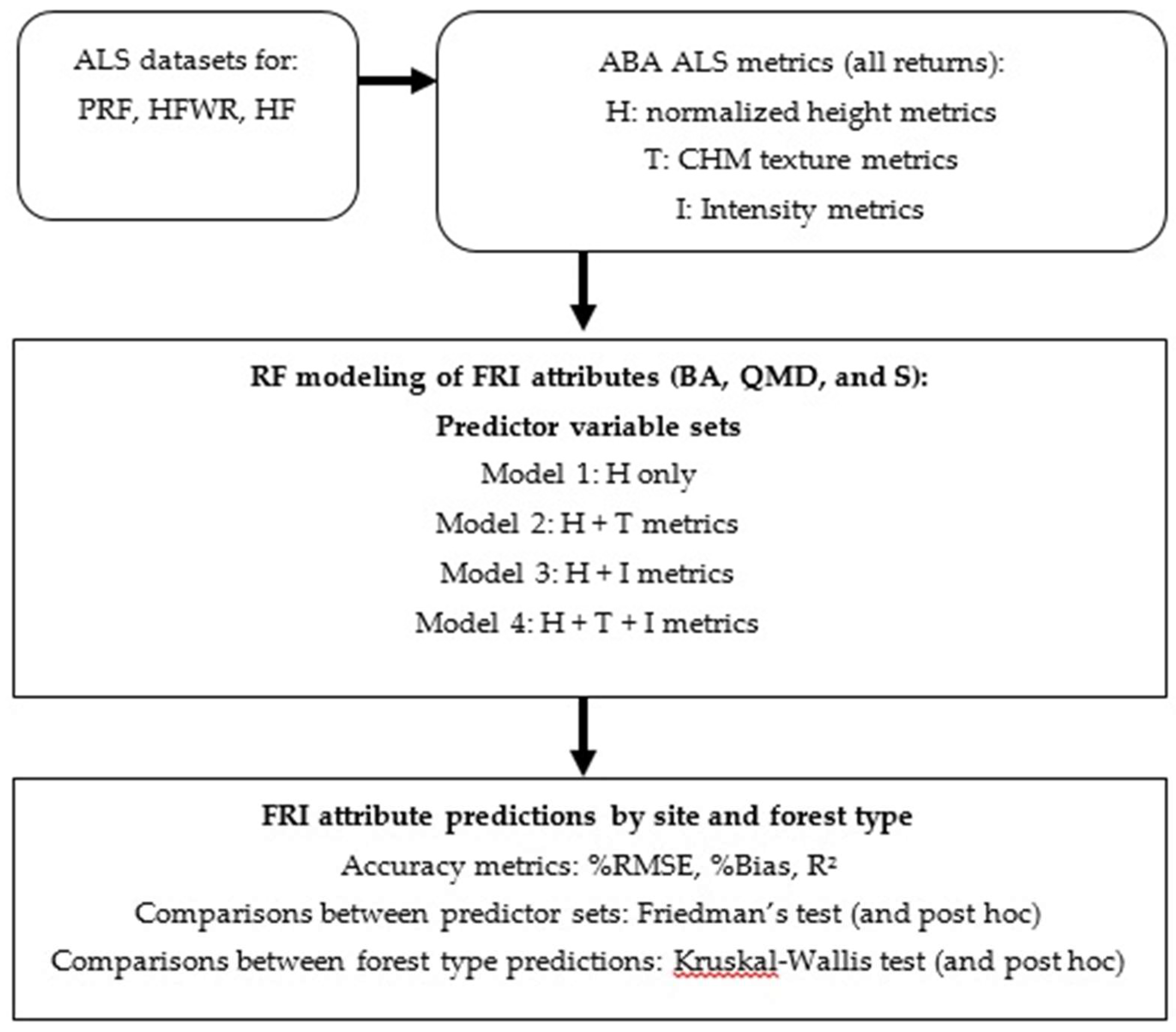
Our major analyses are summarized in Figure 2. First nonparametric models were constructed to predict BA, QMD, and S at our three sites using four different sets of ALS metrics as predictor variables. With the four sets of predictor variables we set out to test whether BA, QMD and S predictions in boreal and GLSL sites improved with additional characterization of the upper canopy (also known as texture) and/or additional characterization of canopy permeability (also known as intensity). We then assessed the performance of these four RF models in each study site and at the forest type level using %RMSE, %Bias, and R2. Lastly, we tested if the prediction errors on the site and forest type level were significantly different from each other using Friedman’s and Kruskal–Wallis tests.
The methods to predict and map FRI attributes vary greatly and range from parametric ordinary least square (OLS) regression to nonparametric approaches such as Random Forests (RF [61]) [26]. There is no consensus on which of these methods performs best as this depends on how model performance is defined, the purpose of the analysis, available resources, data characteristics, and underlying biophysical conditions of the forest [62]. For the operational prediction of FRI attributes, e.g., in Ontario [13,44] and elsewhere [63,64,65], nonparametric machine learning approaches have been shown to offer advantages. These studies found that RF, with its ability to handle complex, high-dimensional interactions between predictors [66], had equivalent results when compared to parametric methods in terms of accuracy and precision of the FRI attributes predicted for a boreal forest in northern Ontario [13]. Penner et al. [13] stated that one important advantage of RF modeling was the use of cross-validation during model development which resulted in relatively robust models. RF’s relative ease of wall-to-wall mapping of the predictions, excluding the need for (i) precise forest-type information at the spatial resolution of the predictive model(s), (ii) forest polygons with tree species information, or (iii) stratifying the [13,65], gives the RF modeling approach a significant advantage from an operational perspective.
Hence, to predict the three FRI attributes over the three different sites we applied RF. In the RF approach, a virtual forest or ensemble of regression trees is built using bootstrapped (with replacement) sample plot calibration data. The ensemble of regression trees is allowed to grow to maximum predictive accuracy [67], while bootstrapping minimizes the correlation between residuals of single trees [68].
We used leave-one-out cross-validation (LOOCV) to assess model performance over the full range of forest conditions at each of the forest sites because plot numbers varied greatly among the three sites and plot numbers were low at PRF. We calculated the average bias (absolute and relative), RMSE (absolute and relative) as a measure of error spread, and the coefficient of determination (R2) to evaluate the predictive performance of the RF models at the site and forest type level. Bias, RMSE and R2 were calculated as follows.
b i a s =   1 N i = 1 N ( y ^ i y i )
b i a s % = b i a s y ¯ × 100
R M S E =   1 N i = 1 N ( y ^ i y i )
R M S E % =   R M S E y ¯ × 100
R 2 = 1 ( y y ¯ ) 2 ( y y ¯ ) 2
where N is the number of validation plots, yi is the observed value for plot i, ŷi is the predicted value for plot I, and ȳ is the mean of the observed variable, i.e., BA, QMD, or S.
To compare the FRI attribute prediction error of the different RF models within each site we used the RMANOVA (repeated-measures analysis of variance) [69]. The nonparametric RMANOVA test, i.e., Friedman’s Test including a post hoc test, evaluates the null hypothesis that the medians of the prediction errors for each of the FRI attributes are the same among the four RF models that used different sets of predictor variables [69]. If significant differences exist, the Wilcoxon–Nemenyi–McDonald–Thompson post hoc test performs a comparison on each paired RF model. We used a nonparametric version of the RMANOVA because not all FRI attributes over the three study sites fulfilled the assumptions of a normal distribution and equal variances of the residuals [69].
To compare the FRI attribute prediction errors at the forest type level, we used the nonparametric Kruskal–Wallis test (including a post hoc test). The Kruskal–Wallis test can be used when groups do not have the same sample sizes [69]. The Kruskal–Wallis test evaluates the null hypothesis that the medians of the FRI attribute prediction errors are the same among the forest types within each of the sites. If significant differences in medians exist among the forest types, the pairwise Mann–Whitney U-test can be used as a post hoc analysis to identify which forest type pairs have significantly different medians. The nonparametric Kruskal–Wallis test was used because not all of the FRI predictions over the forest types fulfilled the assumption of a normal distribution and equal variances of the residuals.
All statistical analyses were performed in R version 3.4.1 [58] using the caret package version 6.0-77 [70] and randomForest package version 4.6-12 [71] to predict FRI variables. A function by Galili [72] was applied to compare the FRI attribute predictions generated with the four different ALS datasets. The kruskal.test and pairwise.wilcox.test functions to perform the Kruskal–Wallis and post hoc tests for the FRI attribute prediction comparisons among forest types are found in the native stats package in R.

3. Results

3.1. FRI Attribute Prediction at the Forest Site Level

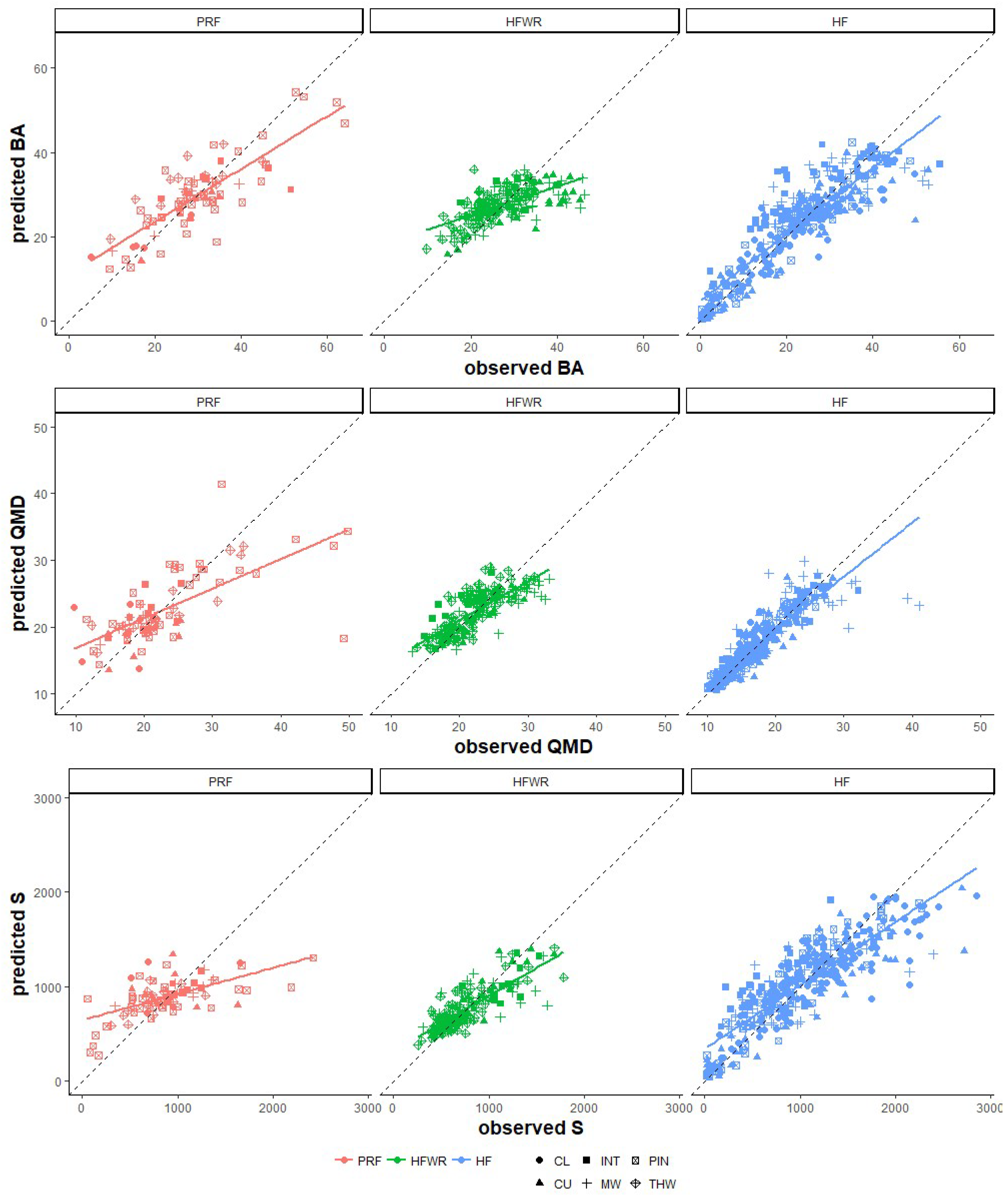
Although the prediction accuracy metrics (i.e., %RMSE, %Bias, and R2) for the four predictor variable sets showed considerable variation over the three forest sites and FRI attributes, some tendencies were observed (Figure 3, Table 4). At all three sites, the addition of texture and/or intensity metrics to the predictor set improved %RMSE, %Bias, and R2. For the PRF, including intensity metrics in the predictor set always improved (i.e., lowered) %RMSE. In HFWR, including texture and intensity metrics resulted in the lowest %RMSE. For HF, the inclusion of texture metrics improved %RMSE more than the inclusion of intensity metrics; however, the lowest %RMSEs in HF for BA, QMD, and S were observed when all predictors were combined. The largest improvements in %RMSE were observed in S predictions for HFWR and PRF (6% and 3.4%, respectively) when intensity metrics were added to the set of predictor variables. In terms of %Bias, the lowest average bias was observed over all three FRI attributes and sites when texture metrics were combined with our baseline predictors, with the exception of BA in PRF where the lowest average bias was observed using only height-based metrics. Figure 3 illustrates that all RF models were on average over-predicting BA, QMD, and S regardless of which predictor variable set was being used, with the exception of QMD predictions in PRF which were on average underpredicted. Patterns in R2 (Table 4) corresponded closely with patterns observed in %RMSE. For PRF, R2‘s for BA, QMD, and S were highest when intensity metrics were included. In HFWR and HF, RF models that included both texture and intensity metrics often resulted in the highest R2 values. The largest improvements in R2 were observed in S predictions when the predictor sets in HFWR and PRF included intensity metrics (0.48 to 0.67 and 0.27 to 0.41, respectively). Overall, S predictions benefited the most by including texture and intensity metrics, particularly for the GLSL forest region sites, whereas BA and QMD predictions show minimal change/improvement, especially in HF.
When prediction accuracy metrics were compared among the three sites, no trends were observed, i.e., %RMSE’s for all FRI attributes were lowest in HFWR, the lowest %Bias values were observed in PRF (BA) and HFWR (QMD and S), and R2’s for all FRI attributes were highest in HF, regardless of which predictor variable sets used. The Friedman’s test indicated that none of the distributions of our FRI prediction errors significantly differed from each other (p > 0.05) (Table 5).

3.2. FRI Attribute Prediction at the Forest Type Level

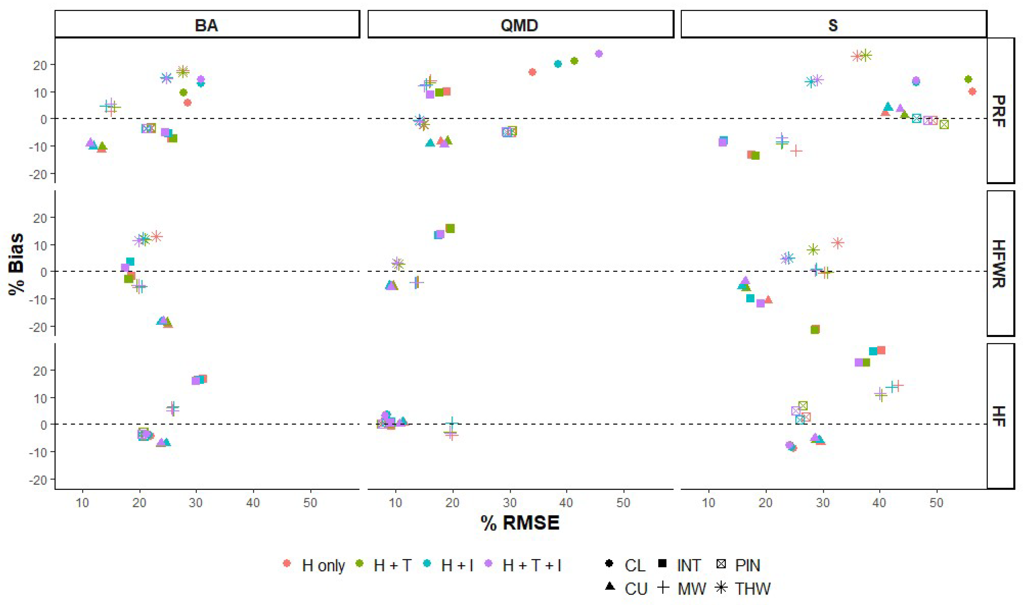
At the forest type level we also observed considerable variation in %RMSE, %Bias, and R2 among FRI attributes and sites (Figure 4 and Figure 5). In PRF and HFWR, we observed the greatest improvements in %RMSE and %Bias in lowland conifers and intolerant and tolerant hardwood forest types when texture and intensity metrics were included in the predictor set. For example, in PRF, %RMSE improved by 10% and 7% in predicted S for lowland conifers and tolerant hardwoods, respectively. In HFWR, %RMSE and %Bias improved in intolerant and tolerant hardwoods by 10% and 9% (%RMSE), respectively, and 10% and 6% (%Bias), respectively, for S predictions. Meanwhile, the least amount of change in %RMSE and %Bias was observed for HF (all forest types show <5% change), when texture and intensity metrics were included.
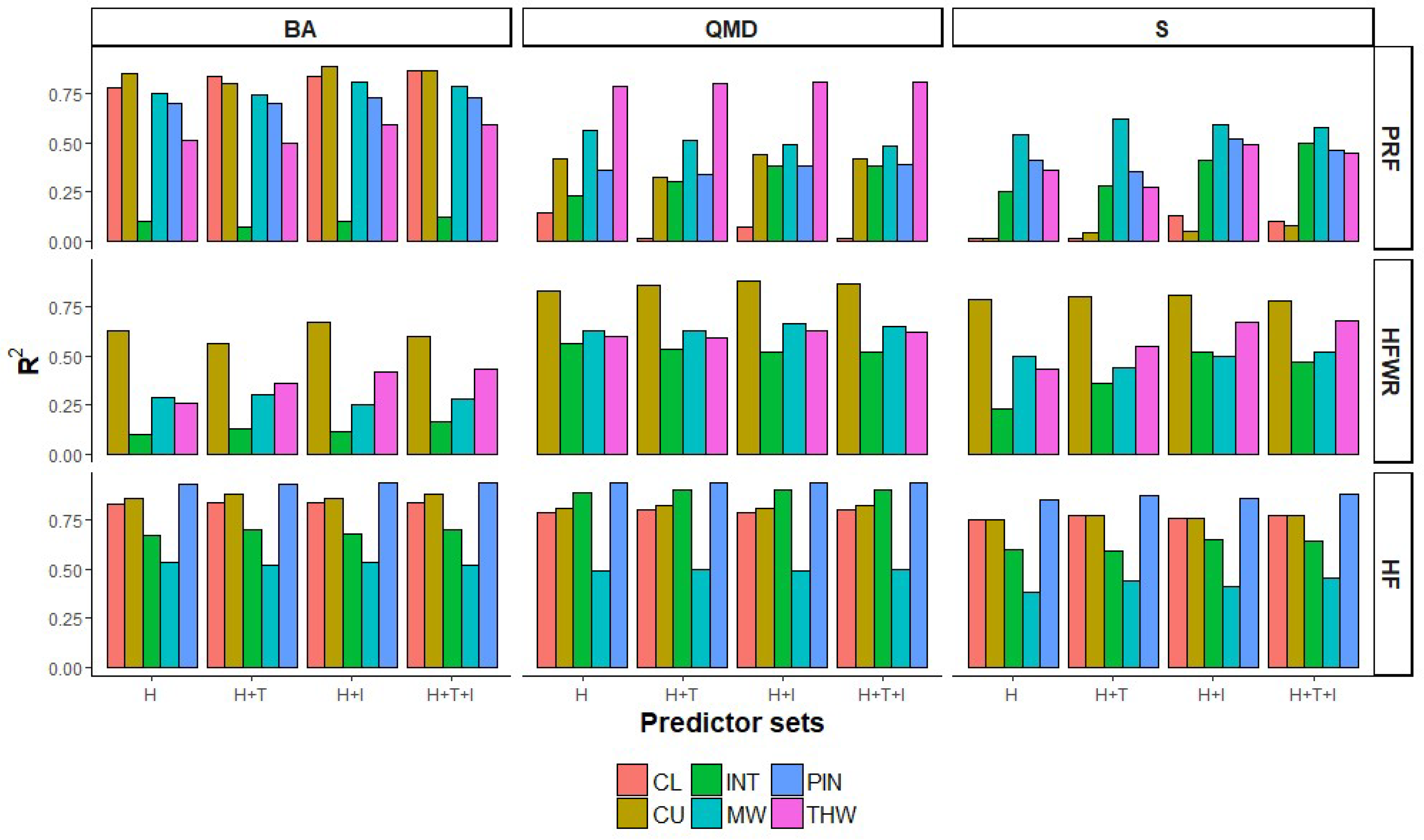
Including texture and intensity metrics in the predictor set also impacted R2 values (Figure 5). Changes in R2 are observed in S predictions for PRF and HFWR, BA predictions for HFWR, and QMD predictions for PRF, but vary among forest types. For example, in PRF we see improvements in R2 in QMD and S predictions in intolerant hardwoods, red/white pines, and tolerant hardwoods, and decreasing R2 values of QMD in lowland conifers. In HFWR, improvements in R2 values were seen in BA and S predictions for intolerant and tolerant hardwoods. Hence, when we combine both site and forest type level results, it appears that changes in site level %RMSE, %Bias, and R2, due to the addition of texture and intensity metrics to the predictor set, are the result of the improvement in some but not all forest types present at a site and that improvements are site and FRI attribute specific.
In terms of comparing prediction accuracy between forest types, we see that in the boreal site (i.e., HF), prediction accuracies for conifer forest types (CL, CU, and PIN) were better than for intolerant hardwoods and mixedwoods for all three FRI attributes. For example, the highest R2 values for BA, QMD, and S were observed in jack pine followed by upland and lowland conifers. In the GLSL forest sites (i.e., HFWR and PRF), such consistent patterns in prediction accuracies among forest types and FRI attributes were not evident, with PRF showing the most variability in prediction accuracy among forest types. For example, for the predictions using all ALS metrics (height-based, texture, and intensity), the differences between the forest types with the lowest and highest %RMSE in PRF were 19.4% (BA), 31.3% (QMD), and 35.4% (S). In contrast, in HFWR and HF the differences in %RMSE between certain forest types were much lower, i.e., 6.7%, 8.6%, and 12.3% in HFWR, and 9.5%, 11.9%, and 15.9% in HF for BA, QMD, and S, respectively. However, no consistency in forest types displaying lowest or highest %RMSE could be determined for any of the sites.
When we tested for differences in BA, QMD and S prediction errors between forest types, all three FRI variables and sites showed significant differences (p < 0.01 to p <= 0.0001) (Figure 6). The Mann–Whitney U post hoc tests indicated that pairwise differences between forest types varied within and between sites for the three FRI attributes. However, in HF and HFWR we observed more significant differences between forest types than in PRF (Table A2).

4. Discussion

Our results demonstrate that FRI attribute predictions improved at all three sites in terms of RMSE, bias, and R2, albeit to varying degrees, when texture and/or intensity metrics were integrated with normalized height metrics derived from ALS data. These findings support previous studies (e.g., [31,33,35,36]). Ozdemir and Donoghue [31] found that the CHM-based texture metrics improved predictions of height, DBH, and crown variability over using point-based ALS metrics alone in their study sites in northeast England. They also noted that improvements in prediction accuracy varied with tree-size diversity indices. Niemie and Vauhkonen [33] tested a wide range of CHM-based texture metrics and found that GLCM texture metrics were one of the texture metrics groups that were moderately successful for predicting VOL, BA, and QMD in a southern boreal forest site in Finland, especially when combined with density metrics derived from the ALS point data. They found, however, that texture metrics predominantly described dominant canopy properties such as total VOL, BA, and QMD, rather than the variability within these properties.
Garcia et al. [35] found that normalized intensity-related metrics provided more accurate estimates of biomass and explained more of the variance in their biomass models in a mixed species Mediterranean forest. Metrics that incorporated intensity at different height percentiles (which can be viewed as a combination of height and intensity information) along with intensity-based measures of canopy closure were selected in their overall and species-specific biomass models. Shang et al. [36] compared the utility of height and intensity metrics for the prediction of size class specific stem densities in the GLSL HFWR site. They found that intensity-based metrics and height percentiles had high RF importance scores for the majority of the size classes and total stem density, indicating their relevance in predicting stem diameter distributions. They contributed this to the fact that the variance of intensity captured the permeability or layering of the canopy which enabled the differentiation between high and low stem density stands. These and other studies [38,39] attributed the improvement in prediction accuracy of forest attributes to the ability of intensity metrics to take into account the amount of foliage, variation in foliage structure, and species composition, aspects that ALS-based height metrics do not necessarily capture.
In our study, at the forest site level, the combination of ALS height-based, texture and intensity metrics (HF and HFWR) or ALS height-based and intensity metrics (PRF) improved the RMSE and R2 of the BA, QMD and S predictions, whereas the addition of texture metrics in almost all sites and for all FRI attributes improved the average bias. Like Ozdemir and Donoghue [31] we also found that improvements in prediction accuracy, due to the added texture and intensity metrics, varied by FRI attribute, e.g., improvements up to 6% RMSE were observed in S predictions, whereas improvements in BA and QMD never exceeded 1.5% RMSE. For all three sites, RF models to predict S were always the weakest models, which may explain why these models gained the most by having texture and intensity metrics included in the predictor sets. Another indicator of the utility of texture and intensity metrics in our FRI attribute predictions was the RF variable importance measure. For the prediction of S, texture (GLCM dissimilarity (HFWR), GLCM entropy (PRF), GLCM correlation (HF)), and intensity (ISD (PRF and HFWR)) metrics were highly ranked in terms of variable importance at all sites. For BA predictions in HFWR, the ISD metric was the second most important metric when all ALS metrics were incorporated in the predictor set. Another study in PRF also found that CHM-derived texture and other metrics (Roughness, Ruggedness, and Variance) were often highly ranked in terms of RF variable importance [52].
Differences in prediction accuracy improvements among the three sites were also observed, with greater changes being observed more frequently in the GLSL (i.e., HFWR and PRF) sites than in the boreal site (i.e., HF). For example, the %RMSE of the S predictions improved by 3.4% in PRF and 6% in HFWR, whereas S predictions in HF improved by 1.7% when texture and intensity metrics were included in the predictor set. Similar to Hollaus et al. [43] and Bouvier et al. [16], we observed better R2 values in the boreal, conifer dominated, forest site for all three FRI attributes than in the broadleaved dominated (HFWR) and more mixed (PRF) GLSL forest sites. One reason for observing better predictive accuracies in both HF and HFWR, compared to the PRF, may be attributed to sample size and sample plot size at each of the forest sites. With 387 sampling plots, HF had the largest number of plots, followed by HFWR with 185, and 84 for PRF. In terms of plot size, HFWR had the largest plot size (2500 m2), followed by PRF (1000 m2) and then HF (400 m2). Shang et al. [73] found that sample plot size had a stronger impact on model performance than the number of plots in their diameter distribution predictions in HFWR. However, Fassnacht et al. [74] found that when a combination of increased plot sizes and reduced number of plots was used, the prediction accuracy benefits of the increased plot size decreased. They attributed this mostly to the decreased model performance of a model calibrated with lower sample sizes. In our study, the 84 sample plots in PRF were unable to cover the full range of stand conditions found in PRF; hence, QMD and S prediction accuracies, in particular, were substantially lower compared to prediction accuracies observed in HFWR and HF. A comparison of prediction accuracies with a previous study in PRF [52], which included 223 field plots (plot size of 625 m2), is inconclusive in terms of attributing the decreased prediction accuracy in PRF to the number of sampling plots only. QMD prediction accuracies showed a %RMSE difference of 7% between their predicted QMD % RMSE (17%) and the %RMSE (25%) found in this study. However, in terms of BA predictions, the %RMSE found in this study (22% RMSE) was better than in theirs (25% RMSE). Differences in ALS sensor, wavelength of the ALS sensors, and ALS-based predictor variable sets used in both studies may also contribute to the differences between these studies. In addition, this study used existing field datasets to calibrate the FRI attribute models and hence some field datasets may have fitted the purpose of this study better than others. For example, in HF, the field data were initially collected to support an OLS modeling approach to predict FRI attributes, and purposely sampled all forest types present in HF. In HFWR, the field data collection focused on upland ecosites, which comprises 90% of the HFWR landscape. Some lowland and less common ecosite types were not represented in their sampling design, explaining the lack of lowland conifer data for this forest site. In PRF, the stratified sampling scheme was based on a principal component analysis of a large set of ALS metrics with the intent to capture a wide range of forest structural conditions and hence did not explicitly focus on sampling all forest types [52]. In addition, only a subset of these plots were remeasured for the 2016 ALS acquisition and used in the analysis presented here. Lastly, since relationships between stand structure and forest attributes are species-dependent, many studies have found that model prediction accuracy decreases in multi- or mixed-species forest stands [2,8,16,75]. However, lower prediction accuracies have also been observed in stands with poorer growth conditions [17] and in forest stands that are more heavily influenced by forest management practices [42]. Among our three sites, structural complexity and species composition were expected to be less variable for the boreal forest site, i.e., HF is largely dominated by conifers (70% versus 30% mixed and intolerant hardwoods) [13], and more complex for the temperate forest sites. In HFWR, however, species composition was fairly homogenous, i.e., the dominant species in almost all plots is sugar maple [45]. Hence prediction accuracies in both HF and HFWR were better than in PRF, which was the most complex forest site in terms of species composition and structure.
An aspect that negatively affected prediction accuracy at all three sites and across all forest types may be attributed to the modeling approach we chose to use in this study. Despite RF’s advantages for wall-to-wall mapping of predicted FRI attributes, the RF approach is also known to underestimate high predicted values and overestimate low predicted values and is not able to extrapolate beyond the range of the training data [25]. This bias is exacerbated when sample size is small [76]. Fundamentally, RF is a nearest neighbor method where observations are predicted using the averages of response values of neighboring observations [77]. Especially in small datasets, data points in the tails of the response variable distribution may differ substantially from its nearest neighbors, which causes the predictions of these data points to move towards the center of the training data, i.e., large response values are underestimated and small values overestimated [76,77]. In our study, this bias was observed in all three sites (Figure 3), but especially in PRF, and also over all forest types . RF bias correction strategies that could potentially improve RF predictions have—as of yet—not been well-studied [76], nor have they been implemented in many of the available RF software packages. Hence, no bias correction of the FRI attribute predictions was performed in this study. However, from an operational forest management perspective, knowledge of the proportion of the landscape that is affected by this bias and the location of the forest stands that are impacted by this bias is important. Coulston et al. [78] proposed a Monte Carlo approach to quantify prediction uncertainty within RF regression models. Maps of such estimates of the RF prediction uncertainty, in addition to the FRI attribute prediction surfaces for each forest sites could subsequently be used to address this.
The %RMSE observed in this study were comparable to other studies that modeled similar FRI attributes at the same forest sites [10,13,44,45,52]. These prediction accuracies were calculated at the plot level (or pixel level once wall-to-wall prediction surfaces of the FRI attributes are generated). For operational forest management, however, prediction accuracies at the stand level, i.e., encompassing several pixels, are more relevant and may very well be lower. Næsset [2,79] found in their two-phase modeling approach of FRI attributes that the standard deviation between predicted and observed plot values were substantially larger than the standard deviations in the same attributes for entire forest stands. At the plot level, FRI attribute predictions can be highly variable, however, once plot estimates are averaged over a stand (encompassing several pixels) the variability is reduced and prediction accuracy improves [79,80,81]. However, Iqbal et al. [81] showed that %Bias increased when prediction accuracies were calculated at the stand level, possibly because at the stand level those errors are more likely to accumulate. For this study we did not have stand level validation data available for all three sites and hence could not test this for our forest sites or test the existence of variability among sites.
Uniform increases or decreases in prediction performances in BA, QMD, and S were not observed when texture and intensity metrics were included in the predictor set. Instead, site level prediction improvements arising due to texture and intensity metrics were observed due to improvements in certain forest types but not in all, i.e., improvements varied by site and FRI attribute. If we focus on the S predictions, as these predictions improved the most by the addition of texture and intensity metrics, these metrics appeared to be most beneficial for forest types whose prediction performances were lower initially, i.e., lowland conifers (from 56.2% to 46.3% RMSE) and tolerant hardwoods (from 35.9% to 27.9% RMSE) in PRF, intolerant (from 28.8% to 17.3% RMSE) and tolerant hardwoods (from 32.6% to 23.5% RMSE) in HFWR, and intolerant hardwoods (from 40.3% to 36.4% RMSE) and mixedwoods (from 43.1% to 40% RMSE) in HF. The variability in prediction accuracy between forest types and the variability in improvement in prediction accuracy within forest types when additional ALS metrics are incorporated has been observed in other studies (e.g., [13,15,16,42]). Næsset [75], Heurich and Thoma [42], and Kotivuori [17] have pointed out that the structural diversity between forest types (in terms of tree species, crown shape and width, canopy cover and layering, etc.) have considerable effects on the ALS-based metrics and hence on FRI attribute predictions. For example, crown shape differences and the different properties of needles and leaves influence the penetration of laser pulses into the canopy surface and hence influence the height distributions calculated from the ALS data [44,76]. In addition, variation in crown width and number of trees, due to differences in site quality, competition and silvicultural practices within different forest types, may greatly affect the relationship between FRI attributes and ALS-based density metrics [75]. For example, many plots classified as tolerant hardwoods (with larger tree crowns and lower stem densities) had lower values for the ALS metrics D7-9 compared to upland and lowland conifer plots (with smaller tree crowns and higher stem densities). It is no surprise that we noticed similar variability in relationships between texture and intensity-based metrics and FRI attributes within the different forest sites and forest types as well. Intensity-based metrics may be able to discriminate between tree species with different leaf angle distributions/orientations, e.g., erectophile versus planophile leaf angle distributions in aspens and maples, respectively. The relationships between ALS metrics and forest type specific FRI attributes, especially for lowland conifers, upland conifers, intolerant hardwoods, and mixedwoods in PRF, should be treated with caution because of the low sample sizes (i.e., <10 sample plots) within these forest types. In addition, some ambiguity existed in the definition of forest types, especially for mixedwoods and hardwoods forest types, which may have affected this relationship. Furthermore, relationships between intensity metrics and the FRI attributes were influenced by the different ranges in intensity values among the three ALS datasets which hampers the interpretation. In order to properly compare and understand the relationship between FRI variables and the intensity metrics, a radiometric correction of the ALS intensity values is required [34]. Since the key input features, such as the range between the sensor and individual returns, required for the radiometric correction procedure were not available for two of our ALS datasets, radiometric correction was not performed. Hence, more research is required to further our understanding of ALS intensity metrics in relation to the FRI variables and their consistency over different forest sites and forest types and across different sensors and acquisition conditions.
Conifer FRI attribute predictions in HF (i.e., boreal) were consistently better, i.e., lower %RMSE, lower %Bias, and higher R2 than in mixedwoods and intolerant hardwoods. For example, jack pine predictions consistently had the best R2 values over all three FRI attributes and mixedwood predictions consistently the worst. This is in line with previous findings [2,41,44,75]. For example, Pitt et al. [44] observed that the quality of FRI attribute predictions varied with forest type and that the largest errors were observed in boreal mixedwoods in HF, regardless of which prediction method used. Contrary to the findings in the boreal zone, Spriggs et al. [45] found that in HFWR, prediction accuracy was better for broadleaved species and postulated that estimation models were most suited to the dominant forest type of a site. In the GLSL forest sites, we did not observe either of these trends consistently over the three FRI attributes and two sites. When we compared Spriggs et al. [45] conifer class to our upland conifer forest type and their broadleaved class to our tolerant hardwood forest type, our BA prediction accuracies at the forest type level were similar, i.e., BA RMSEconifer = 7.39 versus 8.26 m2/ha, RMSEbroadleaved = 5.93 versus 4.72 m2/ha. Hence, in both studies, broadleaved stands had lower RMSEs. However, S predictions between the two studies did not demonstrate this trend as clearly. At the forest type level, Spriggs et al. [45] reported an RMSE of 268 stems/ha in conifer stands versus 156 stems/ha in broadleaved stands whereas in this study the difference was much smaller, i.e., 157 and 151 stems/ha, respectively. Also, in terms of R2, upland conifers performed better than tolerant hardwoods in our study. Spriggs et al. [45] did not include this as one of their accuracy measures. Differences in the prediction modeling approach and how the field data were split in conifer versus broadleaved versus our four forest types may explain the differences in S prediction accuracies found between the two studies.
Zolkos et al. [15] attributed the variability within and between forest types, in part, to the fact that it is possible to have similar forest stand structures yielding different BA, QMD, and S values, while Heurich and Thoma [42] pointed out that silvicultural treatment within forest types affected prediction accuracies. In our study we noticed this within the pine forest types in PRF. Pine forests were extremely diverse as it incorporated pine plantations, stands that have undergone partial harvesting (uniform shelterwood regeneration cuts) and natural unmanaged red pine/white pine stands. For example, Figure 7 shows that within this forest type in PRF, different BA–QMD, BA–S, and QMD–S relationships were observed than for the other forest types across the three sites. For example, the high QMD variance at low BA values is explained by pine plantations having low QMD and seed tree stands having high QMDs. Similarly, many of the normalized height-based ALS metrics had difficulties distinguishing between pine plantations and stands with residual trees remaining after a partial harvest even though these two stand types yield very different QMD and S values, i.e., pine plantations had lower QMDs and higher stem densities compared to partially harvested stands. Some of the texture and intensity-based metrics seemed to better separate plantations, silviculturally-treated, and natural stands; however, the red pine/white pine QMD and S predictions for PRF displayed high %RMSEs and only small changes in prediction accuracy were observed when texture and intensity metrics were included in the predictor sets. To investigate the prediction accuracy in the red pine/white pine forest type in PRF further, we recalculated %RMSE and %Bias when sample plots were split into natural unmanaged and silviculturally-treated plots (plantations and partial harvested stands). Both %RMSE and %Bias were substantially larger in silvicultural treated plots than in natural unmanaged plots for all three FRI attributes, i.e., %RMSEs for natural and silviculturally-treated plots were 19.1% and 29.3% (BA), 13.8% and 42.2% (QMD), and 32.2% and 71.6% (S), respectively and %Bias were −3% and −6% (BA), 1% and −15% (QMD), and 3% and −9% (S), respectively. Prediction accuracies for unmanaged natural plots were closer to the ones found for the tolerant hardwood forest type, whereas the silviculturally-treated plots together with lowland conifers had the lowest prediction accuracies. Woods et al. [10] observed the effect of stand spacing and silvicultural treatments on the prediction accuracies of ALS-based models of FRI attributes for multiple forest sites throughout central Ontario. Similarly, Heurich and Thoma [42] found that selective harvesting in coniferous stands had a negative influence on the prediction accuracies of FRI attributes in the Bavarian Forest National Park in Germany. These studies may indicate that “standard” ALS-based metrics used to predict FRI attributes are not able to sufficiently characterize silviculturally-treated stand conditions. Ayrey and Hayes [82] demonstrated that conditional neural networks (CNN), which use 3D volumetric pixels or voxels derived from the ALS point cloud rather than a set of traditional ALS-based metrics as model input, outperformed RF and linear mixed models for some of their above ground biomass, tree count, and percent conifer predictions. They indicated that some of the features that the CNN uses to make predictions relate to edges, surfaces and possibly branches within the voxelized point cloud, features that ABA- ALS-based metrics do not capture [82]. Their study, however, predicted these attributes over several sites and did not focus on differences in prediction accuracies among different forest types or stand conditions within these sites.
In this study, we have quantified the variability in FRI prediction accuracy between three Ontario forest sites and between the forest types within these sites. However, we acknowledge that additional research is needed to get better insights into the relationships between prediction error and forest types especially in the more complex GLSL.

5. Conclusions

In this study we demonstrate that FRI attribute predictions for BA, QMD, and S over three contrasting Ontario sites improves with the addition of texture and intensity-based ALS metrics (i.e., over using height metrics alone). Although no significant differences between predictions were detected using the nonparametric RMANOVA test at the site level, the nonparametric Kruskal–Wallis test indicates that significant differences exist in prediction errors between the different forest types (p < 0.01 to p ≤ 0.0001). Texture metrics seem more relevant for the boreal site but improvements were relatively small, whereas intensity metrics improved predictions in the GLSL sites, especially in terms of stem density. Since the intensity metrics used in this study were derived from raw ALS intensity data, the impact of intensity normalization/radiometric correction on the model predictions requires further research especially since multiple ALS sensors were used in this study. When we combine site and forest type level results, we demonstrate that improvements in site level predictions, due to the addition of texture and intensity metrics to the ALS predictor set, are the result of changes in some but not all forest types present at a site and that these changes are site and FRI attribute specific. Our study found that boreal site prediction accuracies were most consistent among FRI attributes and forest types, and conform to other studies performed in the boreal forest zone. Such patterns in prediction accuracy among forest types and FRI attributes was not observed in the GLSL sites. Varied silvicultural treatments for the pine forest types (i.e., pine plantations, silviculturally-treated stands, and natural pine stands) in PRF created a varied set of forest structures over time. The impact of these treatments was especially observed on QMD and S predictions in this forest type.

Author Contributions

All authors were involved in the conceptualization of this research. K.V.E., P.T., M.W., J.C., and T.J. contributed to the data processing, data analysis, and write-up. M.W., J.C., and T.J. provided access to field and ALS data. All authors contributed to the interpretation and revisions of the manuscript. All authors read and approved the final manuscript.

Funding

This research was funded by AWARE (Assessment of Wood Attributes from Remote Sensing NSERC CRDPJ462973-14; grantee Prof Nicholas Coops, UBC), in collaboration with the Canadian Wood Fibre Centre (CWFC), FP-Innovations and Tembec Incorporated. J.C. was funded by the NRCAN ecoENERGY program and HFWR.

Acknowledgments

We want to acknowledge Petawawa Research Forest, Haliburton Forest and Wildlife Reserve, and Hearst Forest Management Inc., for sharing their data. Special thanks to the field assistants at PRF, HFWR, and HF, as well as to D. Pitt for his comments and suggestions on earlier versions of this manuscript.

Conflicts of Interest

The authors declare no conflicts of interest. The funders had no role in the design of the study; in the collection, analyses, or interpretation of data; in the writing of the manuscript, and in the decision to publish the results.

Appendix A

Table A1. List of the set of ALS metrics used in this study.
ALS Metrics:
H-only
DescriptionALS Metrics: TextureDescription
HMAX Maximum (m)CHM-GLCM homogeneityGLCM contrast texture metrics
HMEAN Mean (m)CHM-GLCM contrastGLCM contrast texture metrics
HSDStandard deviation (m) CHM-GLCM dissimilarityGLCM contrast texture metrics
HCVCoefficient of variation (m)CHM-GLCM angular second momentGLCM orderliness texture metrics
HSKEWSkewnessCHM-GLCM entropyGLCM orderliness texture metrics
HKURTOSIS KurtosisCHM-GLCM meanGLCM descriptive statistics texture metrics
P10–P90Height percentiles (m)CHM-GLCM varianceGLCM descriptive statistics texture metrics
D1–D9Cumulative percentage of returns in the nth of 10 equally-spaced height intervals (%)CHM-GLCM correlationGLCM descriptive statistics texture metrics
ALS metrics:
Intensity
Description
DANumber of first returns/total number of returnsIMAXMaximum (ρ)
PFPercentage of returns reaching 2 m (%)IMEANMean (ρ)
VDRVertical distribution ratio [83]ITOTTotal
VCIVertical complexity index [84]ISDStandard deviation (ρ)
LAD.CVCoefficient of variation of the LAD profile (m2/m2) [16]ICVCoefficient of variation (ρ)
ISKEWSkewness
IKURTOSISKurtosis
IZP10-IZP90Cumulative intensity at the nth height percentile (ρ)
Table A2. Forest type prediction error differences between the RF models (p-values of the prediction error differences between forest types were acquired using the unpaired nonparametric Kruskal–Wallis test, including Mann–Whitney U post hoc tests).
FRIFTPRFHAFHEF
BAALL************
PIN****
MW*** **** ****
INT***NSNS ***NS ********
CU*********** ************NS********
CL*NSNSNS**** NS*********
THWPINMWINTCUTHWMWINTPINMWINTCU
QMDALL************
PINNS
MW******* **** *
INT*****NS ******** NS*
CU********* ****NS****NS*NS
CL****NSNS** *************
THWPINMWINTCUTHWMWINTPINMWINTCU
SALL**********
PIN*
MW****** * ****
INT********NS ******** ********
CUNSNS**** ********************
CLNSNSNSNSNS *************
THWPINMWINTCUTHWMWINTPINMWINTCU
1 NS: p > 0.05; *: p ≤ 0.05, **: p ≤ 0.01; ***: p ≤ 0.001; ****: p ≤ 0.0001.

References

  1. Lefsky, M.A.; Cohen, W.B.; Parker, G.G.; Harding, D.J. Lidar Remote Sensing for Ecosystem Studies. Bioscience 2002, 52, 19. [Google Scholar] [CrossRef] [Green Version]
  2. Næsset, E.; Gobakken, T.; Holmgren, J.; Hyyppä, H.; Hyyppä, J.; Maltamo, M.; Nilsson, M.; Olsson, H.; Persson, Å.; Söderman, U. Laser Scanning of Forest Resources: The Nordic Experience. Scand. J. For. Res. 2004, 19, 482–499. [Google Scholar] [CrossRef]
  3. Nilsson, M.; Nordkvist, K.; Jonzén, J.; Lindgren, N.; Axensten, P.; Wallerman, J.; Egberth, M.; Larsson, S.; Nilsson, L.; Eriksson, J.; et al. A Nationwide Forest Attribute Map of Sweden Derived Using Airborne Laser Scanning Data and Field Data from the National Forest Inventory. Remote Sens. Environ. 2017, 194, 447–454. [Google Scholar] [CrossRef]
  4. Kandare, K.; Dalponte, M.; Ørka, H.O.; Frizzera, L.; Næsset, E. Prediction of Species-Specific Volume Using Different Inventory Approaches by Fusing Airborne Laser Scanning and Hyperspectral Data. Remote Sens. 2017, 9, 400. [Google Scholar] [CrossRef]
  5. Gobakken, T.; Bollandsås, O.M.; Næsset, E. Comparing Biophysical Forest Characteristics Estimated from Photogrammetric Matching of Aerial Images and Airborne Laser Scanning Data. Scand. J. For. Res. 2015, 30, 73–86. [Google Scholar] [CrossRef]
  6. Wulder, M.A.; Coops, N.C.; Hudak, A.T.; Morsdorf, F.; Nelson, R.F.; Newnham, G.J.; Vastaranta, M. Status and Prospects for LiDAR Remote Sensing of Forested Ecosystems. Can. J. Remote Sens. 2013, 39, S1–S5. [Google Scholar] [CrossRef]
  7. Lim, K.; Treitz, P.; Wulder, M.; St-Onge, B.; Flood, M. LiDAR Remote Sensing of Forest Structure. Prog. Phys. Geogr. 2003, 27, 88–106. [Google Scholar] [CrossRef]
  8. Lefsky, M.A.; Hudak, A.T.; Cohen, W.B.; Acker, S.A. Geographic Variability in Lidar Predictions of Forest Stand Structure in the Pacific Northwest. Remote Sens. Environ. 2005, 95, 532–548. [Google Scholar] [CrossRef]
  9. Næsset, E. Airborne Laser Scanning as a Method in Operational Forest Inventory: Status of Accuracy Assessments Accomplished in Scandinavia. Scand. J. For. Res. 2007, 7581. [Google Scholar] [CrossRef]
  10. Woods, M.E.; Lim, K.; Treitz, P.M. Predicting Forest Stand Variables from LiDAR Data in the Great Lakes—St Lawrence Forest of Ontario. For. Chron. 2008, 84, 827–839. [Google Scholar] [CrossRef]
  11. Asner, G.P.; Mascaro, J.; Muller-Landau, H.; Vielledent, G.; Vaudry, R.; Rasamoelina, M.; Hall, J.S.; Van Breugel, M. A Universal Airborne LiDAR Approach for Tropical Forest Carbon Mapping. Oecologia 2012, 168, 1147–1160. [Google Scholar] [CrossRef] [PubMed]
  12. Woods, M.; Pitt, D.; Penner, M.; Lim, K.; Nesbitt, D.; Etheridge, D.; Treitz, P. Operational Implementation of a LiDAR Inventory in Boreal Ontario. For. Chron. 2011, 87, 512–528. [Google Scholar] [CrossRef]
  13. Penner, M.; Pitt, D.G.; Woods, M.E. Parametric vs. Nonparametric LiDAR Models for Operational Forest Inventory in Boreal Ontario. Can. J. Remote Sens. 2013, 39, 426–443. [Google Scholar] [CrossRef]
  14. Silva, C.A.; Klauberg, C.; Hudak, A.T.; Vierling, L.A.; Liesenberg, V.; Carvalho, S.P.C.E.; Rodriguez, L.C.E. A Principal Component Approach for Predicting the Stem Volume in Eucalyptus Plantations in Brazil Using Airborne LiDAR Data. Forestry 2016, 89, 422–433. [Google Scholar] [CrossRef]
  15. Zolkos, S.G.; Goetz, S.J.; Dubayah, R. A Meta-Analysis of Terrestrial Aboveground Biomass Estimation Using Lidar Remote Sensing. Remote Sens. Environ. 2013, 128, 289–298. [Google Scholar] [CrossRef]
  16. Bouvier, M.; Durrieu, S.; Fournier, R.A.; Renaud, J. Generalizing Predictive Models of Forest Inventory Attributes Using an Area-Based Approach with Airborne LiDAR Data. Remote Sens. Environ. 2015, 156, 322–334. [Google Scholar] [CrossRef]
  17. Kotivuori, E.; Korhonen, L.; Packalen, P. Nationwide Airborne Laser Scanning Based Models for Volume, Biomass and Dominant Height in Finland. Silva Fenn. 2016, 50, 1–28. [Google Scholar] [CrossRef]
  18. Chen, Q. Retrieving Vegetation Height of Forests and Woodlands over Mountainous Areas in the Pacific Coast Region Using Satellite Laser Altimetry. Remote Sens. Environ. 2010, 114, 1610–1627. [Google Scholar] [CrossRef]
  19. Moser, P.; Vibrans, A.C.; Mcroberts, R.E.; Næsset, E.; Gobakken, T.; Chirici, G.; Mura, M.; Marchetti, M. Methods for Variable Selection in LiDAR-Assisted Forest Inventories. Forestry 2016, 90, 1–13. [Google Scholar] [CrossRef]
  20. Magnussen, S.; Næsset, E.; Gobakken, T.; Frazer, G. A Fine-Scale Model for Area-Based Predictions of Tree-Size-Related Attributes Derived from LiDAR Canopy Heights. Scand. J. For. Res. 2012, 27, 312–322. [Google Scholar] [CrossRef]
  21. Guyon, I.; Elisseeff, A. An Introduction to Variable and Feature Selection. J. Mach. Learn. Res. 2003, 3, 1157–1182. [Google Scholar] [CrossRef]
  22. Khan, J.A.; Van Aelst, S.; Zamar, R.H. Robust Linear Model Selection Based on Least Angle Regression on Least Angle Regression. J. Am. Stat. Assoc. 2007, 102, 1289–1299. [Google Scholar] [CrossRef]
  23. Kohavi, R.; Sommerfield, D. Feature Subset Selection Using the Wrapper Method: Overfitting and Dynamic Search Space Topology. In Proceedings of the 1st International Conference Knowledge Discovery Data Mining, Montreal, QC, Canada, 20–21 August 1995; pp. 192–197. [Google Scholar]
  24. Dos Santos, E.M.; Sabourin, R.; Maupin, P. Overfitting Cautious Selection of Classifier Ensembles with Genetic Algorithms. Inf. Fusion 2009, 10, 150–162. [Google Scholar] [CrossRef]
  25. White, J.C.; Wulder, M.A.; Varhola, A.; Vastaranta, M.; Coops, N.C.; Cook, B.D.; Pitt, D.; Woods, M. A Best Practices Guide for Generating Forest Inventory Attributes from Airborne Laser Scanning Data Using an Area-Based Approach; Information Report FI-X-010; Natural Resources Canada, Canadian Forest Service, Canadian Wood Fibre Centre: Victoria, BC, Canada, 2013. [Google Scholar]
  26. White, J.C.; Tompalski, P.; Vastaranta, M.; Wulder, M.A.; Saarinen, N.; Stepper, C.; Coops, N.C. A Model Development and Application Guide for Generating an Enhanced Forest Inventory Using Airborne Laser Scanning Data and an Area-Based Approach; Information Report FI-X-018; Natural Resources Canada, Canadian Forest Service, Canadian Wood Fibre Centre: Victoria, BC, Canada, 2017. [Google Scholar]
  27. Franklin, S.E.; Wulder, M.A.; Gerylo, G.R. Texture Analysis of IKONOS Panchromatic Data for Douglas-Fir Forest Age Class Separability in British Columbia. Int. J. Remote Sens. 2001, 22, 2627–2632. [Google Scholar] [CrossRef]
  28. Tuominen, S.; Pekkarinen, A. Performance of Different Spectral and Textural Aerial Photograph Features in Multi-Source Forest Inventory. Remote Sens. Environ. 2005, 94, 256–268. [Google Scholar] [CrossRef]
  29. Vauhkonen, J.; Tokola, T.; Maltamo, M.; Packalén, P. Effects of Pulse Density on Predicting Characteristics of Individual Trees of Scandinavian Commercial Species Using Alpha Shape Metrics Based on Airborne Laser Scanning Data. Can. J. Remote Sens. 2008, 34, S441–S459. [Google Scholar] [CrossRef]
  30. Pippuri, I.; Kallio, E.; Maltamo, M.; Peltola, H.; Packalén, P. Exploring Horizontal Area-Based Metrics to Discriminate the Spatial Pattern of Trees and Need for First Thinning Using Airborne Laser Scanning. Forestry 2012, 85, 305–314. [Google Scholar] [CrossRef]
  31. Ozdemir, I.; Donoghue, D.N.M. Modelling Tree Size Diversity from Airborne Laser Scanning Using Canopy Height Models with Image Texture Measures. For. Ecol. Manag. 2013, 295, 28–37. [Google Scholar] [CrossRef]
  32. Packalen, P.; Vauhkonen, J.; Kallio, E.; Peuhkurinen, J.; Pitkänen, J.; Pippuri, I.; Strunk, J.; Maltamo, M. Predicting the Spatial Pattern of Trees by Airborne Laser Scanning. Int. J. Remote Sens. 2013, 34, 5154–5165. [Google Scholar] [CrossRef]
  33. Niemi, M.T.; Vauhkonen, J. Extracting Canopy Surface Texture from Airborne Laser Scanning Data for the Supervised and Unsupervised Prediction of Area-Based Forest Characteristics. Remote Sens. 2016, 8, 582. [Google Scholar] [CrossRef]
  34. Yan, W.Y.; Shaker, A. Reduction of Striping Noise in Overlapping LiDAR Intensity Data by Radiometric Normalization. Int. J. Digit. Earth 2016, 9, 649–661. [Google Scholar] [CrossRef]
  35. García, M.; Riaño, D.; Chuvieco, E.; Danson, F.M. Estimating Biomass Carbon Stocks for a Mediterranean Forest in Central Spain Using LiDAR Height and Intensity Data. Remote Sens. Environ. 2010, 114, 816–830. [Google Scholar] [CrossRef]
  36. Shang, C.; Treitz, P.; Caspersen, J.; Jones, T. Estimating Stem Diameter Distributions in a Management Context for a Tolerant Hardwood Forest Using ALS Height and Intensity Data. Can. J. Remote Sens. 2017, 43, 79–94. [Google Scholar] [CrossRef]
  37. Donoghue, D.N.M.; Watt, P.J.; Cox, N.J.; Wilson, J. Remote Sensing of Species Mixtures in Conifer Plantations Using LiDAR Height and Intensity Data. Remote Sens. Environ. 2007, 110, 509–522. [Google Scholar] [CrossRef]
  38. Hopkinson, C.; Chasmer, L. Testing LiDAR Models of Fractional Cover across Multiple Forest Ecozones. Remote Sens. Environ. 2009, 113, 275–288. [Google Scholar] [CrossRef]
  39. Morsdorf, F.; Mårell, A.; Koetz, B.; Cassagne, N.; Pimont, F.; Rigolot, E.; Allgöwer, B. Discrimination of Vegetation Strata in a Multi-Layered Mediterranean Forest Ecosystem Using Height and Intensity Information Derived from Airborne Laser Scanning. Remote Sens. Environ. 2010, 114, 1403–1415. [Google Scholar] [CrossRef]
  40. Packalén, P.; Maltamo, M. The K-MSN Method for the Prediction of Species-Specific Stand Attributes Using Airborne Laser Scanning and Aerial Photographs. Remote Sens. Environ. 2007, 109, 328–341. [Google Scholar] [CrossRef]
  41. Peuhkurinen, J.; Maltamo, M.; Malinen, J. Estimating Species-Specific Diameter Distributions and Saw Log Recoveries of Boreal Forests from Airborne Laser Scanning Data and Aerial Photographs: A Distribution-Based Approach. Silva Fenn. 2008, 42, 625–641. [Google Scholar] [CrossRef]
  42. Heurich, M.; Thoma, F. Estimation of Forestry Stand Parameteris Using Laser Scanning Data in Temperate, Structurally Rich Natural European Beech (Fagus sylvatica) and Norway Spruce (Picea abies) Forests. Forestry 2008, 81, 645–661. [Google Scholar] [CrossRef]
  43. Hollaus, M.; Dorigo, W.; Wagner, W.; Schadauer, K.; Höfle, B.; Maier, B. Operational Wide-Area Stem Volume Estimation Based on Airborne Laser Scanning and National Forest Inventory Data. Int. J. Remote Sens. 2009, 30, 5159–5175. [Google Scholar] [CrossRef]
  44. Pitt, D.G.; Woods, M.; Penner, M. A Comparison of Point Clouds Derived from Stereo Imagery and Airborne Laser Scanning for the Area—Based Estimation of Forest Inventory Attributes in Boreal Ontario. Can. J. Remote Sens. 2014, 40, 214–232. [Google Scholar] [CrossRef]
  45. Spriggs, R.; Coomes, D.; Jones, T.; Caspersen, J.; Vanderwel, M. An Alternative Approach to Using LiDAR Remote Sensing Data to Predict Stem Diameter Distributions across a Temperate Forest Landscape. Remote Sens. 2017, 9, 944. [Google Scholar] [CrossRef]
  46. Nord-Larsen, T.; Schumacher, J. Estimation of Forest Resources from a Country Wide Laser Scanning Survey and National Forest Inventory Data. Remote Sens. Environ. 2012, 119, 148–157. [Google Scholar] [CrossRef]
  47. Ekstrom, B. Forest Management Plan for the Hearst Forest; Report 2007-2017-SFL 550053; Hearst Forest Management Inc.: Hearst, ON, Canada, 2007. [Google Scholar]
  48. Carleton, T.J. Old Growth in the Great Lakes Forest. Environ. Rev. 2003, 11, S115–S134. [Google Scholar] [CrossRef]
  49. Watkins, L. The Forest Resources of Ontario 2011; Marie: Sault Ste, ON, Canada, 2011. [Google Scholar]
  50. Mrosek, T.; Balsillie, D.; Schleifenbaum, P. Field Testing of a Criteria and Indicators System for Sustainable Forest Management at the Local Level. Case Study Results Concerning the Sustainability of the Private Forest Haliburton Forest and Wild Life Reserve in Ontario, Canada. For. Policy Econ. 2006, 8, 593–609. [Google Scholar] [CrossRef]
  51. Vanderwel, M.C.; Thorpe, H.C.; Shuter, J.L.; Caspersen, J.P.; Thomas, S.C. Contrasting Downed Woody Debris Dynamics in Managed and Unmanaged Northern Hardwood Stands. Can. J. For. Res. 2008, 38, 2850–2861. [Google Scholar] [CrossRef]
  52. Penner, M.; Woods, M. LiDAR Stand-Level Predictions for the PRF; Unpublished work; Ontario Ministry of Natural Resources and Forestry: Peterborough, ON, Canada, 2015. [Google Scholar]
  53. Spriggs, R.A.; Vanderwel, M.C.; Jones, T.A.; Caspersen, J.P.; Coomes, D.A. A Simple Area-Based Model for Predicting Airborne LiDAR First Returns from Stem Diameter Distributions: An Example Study in an Uneven-Aged, Mixed Temperate Forest. Can. J. For. Res. 2015, 45, 1338–1350. [Google Scholar] [CrossRef]
  54. Hopkinson, C. The Influence of Flying Altitude, Beam Divergence, and Pulse Repetition Frequency on Laser Pulse Return Intensity and Canopy Frequency Distribution. Can. J. Remote Sens. 2007, 33, 312–324. [Google Scholar] [CrossRef]
  55. Kashani, A.G.; Olsen, M.J.; Parrish, C.E.; Wilson, N. A Review of LIDAR Radiometric Processing: From Ad Hoc Intensity Correction to Rigorous Radiometric Calibration. Sensors 2015, 15, 28099–28128. [Google Scholar] [CrossRef] [PubMed] [Green Version]
  56. Haralick, R.M. Statistical Image Texture Analysis. In Handbook of Pattern Recognition and Image Processing; Young, T.Y., Fu, K.S., Eds.; Academic press: New York, NY, USA, 1986; pp. 247–279. [Google Scholar]
  57. Hall-Beyer, M. Practical Guidelines for Choosing GLCM Textures to Use in Landscape Classification Tasks over a Range of Moderate Spatial Scales. Int. J. Remote Sens. 2017, 38, 1312–1338. [Google Scholar] [CrossRef]
  58. R Development Core Team. R: A Language and Environment for Statistical Computing; R Foundation for Statistical Computing: Vienna, Austria, 2015. [Google Scholar]
  59. Roussel, J.; Auty, D. lidR: Airborne LiDAR Data Manipulations and Visualisation for Forestry Applications. Available online: http://cran.r-project.org/package=lidR (accessed on 1 August 2018).
  60. Trimble. ECognition® Developer 9.0; Trimble: Munich, Germany, 2014. [Google Scholar]
  61. Breiman, L. Statistical Modeling: The Two Cultures. Stat. Sci. 2001, 16, 199–215. [Google Scholar] [CrossRef]
  62. Brosofske, K.D.; Froese, R.E.; Falkowski, M.J.; Banskota, A. A Review of Methods for Mapping and Prediction of Inventory Attributes for Operational Forest Management. For. Sci. 2014, 60, 1–24. [Google Scholar] [CrossRef]
  63. Stepper, C.; Straub, C.; Pretzsch, H. Using Semi-Global Matching Point Clouds to Estimate Growing Stock at the Plot and Stand Levels: Application for a Broadleaf-Dominated Forest in Central Europe. Can. J. For. Res. 2015, 45, 111–123. [Google Scholar] [CrossRef]
  64. White, J.C.; Arnett, J.T.T.R.; Wulder, M.A.; Tompalski, P.; Coops, N.C. Evaluating the Impact of Leaf-on and Leaf-off Airborne Laser Scanning Data on the Estimation of Forest Inventory Attributes with the Area-Based Approach. Can. J. For. Res. 2015, 45, 1498–1513. [Google Scholar] [CrossRef]
  65. Immitzer, M.; Stepper, C.; Böck, S.; Straub, C.; Atzberger, C. Use of WorldView-2 Stereo Imagery and National Forest Inventory Data for Wall-to-Wall Mapping of Growing Stock. For. Ecol. Manag. 2016, 359, 232–246. [Google Scholar] [CrossRef]
  66. Evans, J.S.; Murphy, M.A.; Holden, Z.A.; Cushman, S.A. Modeling Species Distribution and Change Using Random Forest. In Predictive Species and Habitat Modeling in Landscape Ecology: Concepts and Applications; Drew, C.A., Wiersma, Y.F., Huettmann, F., Eds.; Springer Science+Business Media: Berlin, Germany, 2011; pp. 1–313. [Google Scholar] [CrossRef]
  67. Breiman, L. Random Forests. Mach. Learn. 2001, 45, 5–32. [Google Scholar] [CrossRef] [Green Version]
  68. Segal, M.R. Machine Learning Benchmarks and Random Forest Regression; Center for Bioinformatics and Molucular Biostatistics, UCSF: San Francisco, CA, USA, 2003; Available online: https://escholarship.org/uc/item/35x3v9t4 (accessed on 1 August 2018).
  69. Hollander, M.; Wolfe, D.A. Nonparametric Statistical Methods, 2nd ed.; John Wiley & Sons Inc.: Hoboken, NJ, USA, 1999. [Google Scholar]
  70. Kuhn, M. Building Predictive Models in R Using the Caret Package. J. Stat. Softw. 2008, 28, 1–26. [Google Scholar] [CrossRef]
  71. Liaw, A.; Wiener, M. randomForest: Breiman and Cutler’s Random Forests for Classification and Regression. Available online: http://cran.r-project.org/package=randomForest (accessed on 1 August 2018).
  72. Galili, T. Post hoc analysis for Friedman’s Test (R code). Available online: https://www.r-statistics.com/2010/02/post (accessed on 1 September 2018).
  73. Shang, C.; Jones, T.A.; Treitz, P.M. Effect of Size and Number of Calibration Plots on the Estimation of Stem Diameter Distributions Using Airborne Laser Scanning. In Proceedings of the International Geoscience and Remote Sensing Symposium (IGARSS), Beijing, China, 10–15 July 2016; pp. 1753–1756. [Google Scholar]
  74. Fassnacht, F.E.; Latifi, H.; Hartig, F. Using Synthetic Data to Evaluate the Benefits of Large Field Plots for Forest Biomass Estimation with LiDAR. Remote Sens. Environ. 2018, 213, 115–128. [Google Scholar] [CrossRef]
  75. Næsset, E. Practical Large-Scale Forest Stand Inventory Using a Small-Footprint Airborne Scanning Laser. Scand. J. For. Res. 2004, 19, 164–179. [Google Scholar] [CrossRef]
  76. Xu, R. Improvements to Random Forest Methodology. Ph.D. Thesis, Iowa State University, Ames, IA, USA, 2013. [Google Scholar]
  77. Zhang, G.; Lu, Y. Bias-Corrected Random Forests in Regression. J. Appl. Stat. 2012, 39, 151–160. [Google Scholar] [CrossRef]
  78. Coulston, J.W.; Blinn, C.E.; Thomas, V.A.; Wynne, R.H. Approximating Prediction Uncertainty for Random Forest Regression Models. Photogramm. Eng. Remote Sens. 2016, 82, 189–197. [Google Scholar] [CrossRef]
  79. Næsset, E. Predicting Forest Stand Characteristics with Airborne Scanning Laser Using a Practical Two-Stage Procedure and Field Data. Remote Sens. Environ. 2002, 80, 88–99. [Google Scholar] [CrossRef]
  80. Bohlin, J.; Wallerman, J.; Fransson, J.E.S. Forest Variable Estimation Using Photogrammetric Matching of Digital Aerial Images in Combination with a High-Resolution DEM. Scand. J. For. Res. 2012, 27, 692–699. [Google Scholar] [CrossRef]
  81. Iqbal, I.A.; Musk, R.A.; Osborn, J.; Stone, C.; Lucieer, A. A Comparison of Area-Based Forest Attributes Derived from Airborne Laser Scanner, Small-Format and Medium-Format Digital Aerial Photography. Int. J. Appl. Earth Obs. Geoinf. 2019, 76, 231–241. [Google Scholar] [CrossRef]
  82. Ayrey, E.; Hayes, D.J. The Use of Three-Dimensional Convolutional Neural Networks to Interpret LiDAR for Forest Inventory. Remote Sens. 2018, 10, 649. [Google Scholar] [CrossRef]
  83. Goetz, S.; Steinberg, D.; Dubayah, R.; Blair, B. Laser Remote Sensing of Canopy Habitat Heterogeneity as a Predictor of Bird Species Richness in an Eastern Temperate Forest, USA. Remote Sens. Environ. 2007, 108, 254–263. [Google Scholar] [CrossRef]
  84. Van Ewijk, K.Y.; Randin, C.F.; Treitz, P.M.; Scott, N.A. Predicting Fine-Scale Tree Species Abundance Patterns Using Biotic Variables Derived from LiDAR and High Spatial Resolution Imagery. Remote Sens. Environ. 2014, 150, 120–131. [Google Scholar] [CrossRef]
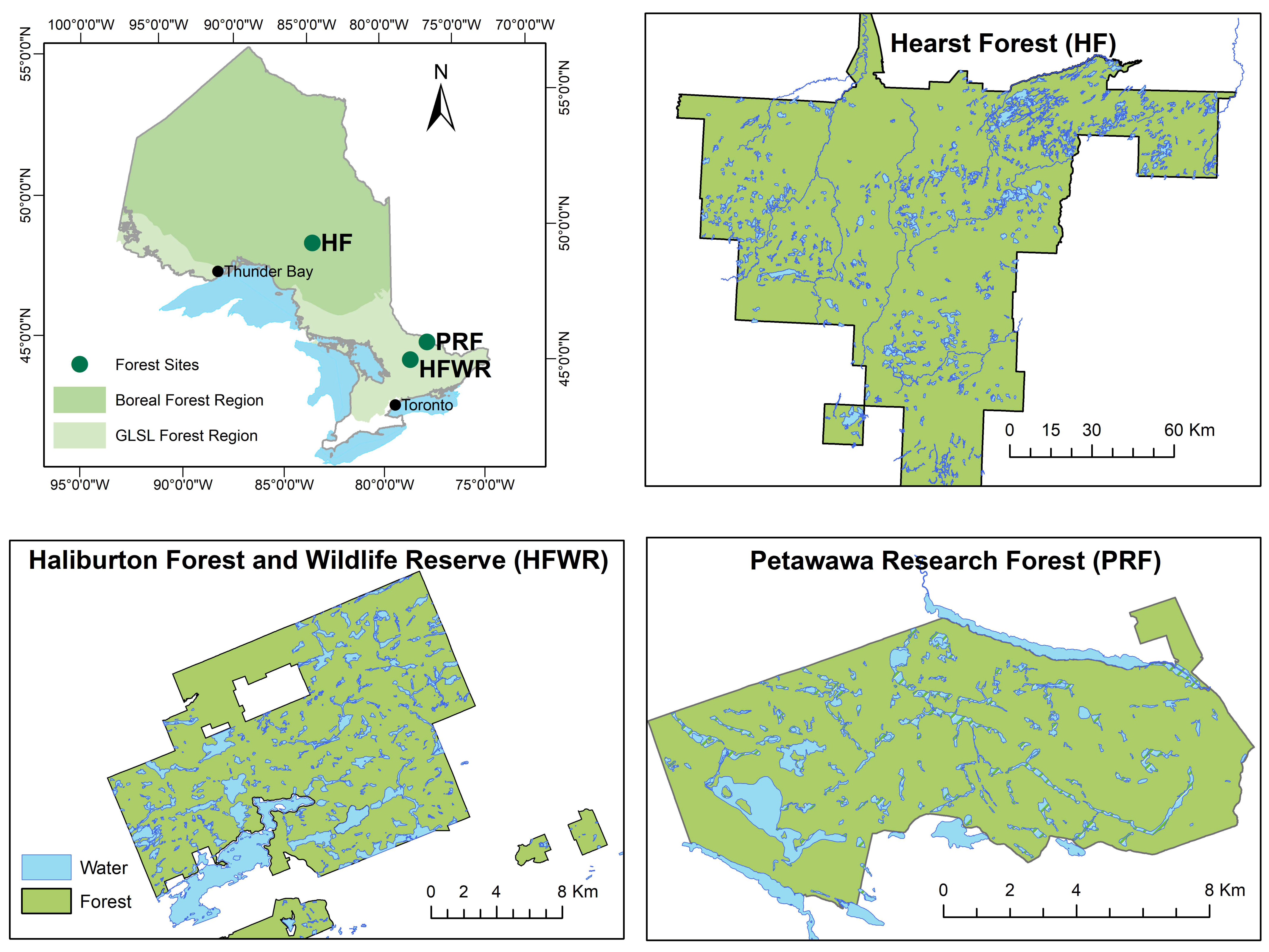
Figure 1. The three study sites in Ontario, Canada.
Forests 10 00226 g001
Figure 2. A flow diagram of the methods used in this study.
Forests 10 00226 g002
Figure 3. FRI predictive models for BA, QMD, and S for each of the sites developed using the RF model including all ALS metrics (z, texture and intensity) and leave-one-out cross-validation. Linear fitted lines by site and the 1:1 line are added to show the different model fits by forest site.
Forests 10 00226 g003
Figure 4. %RMSE and %Bias of the RF models using different predictor variable sets (H only: normalized height metrics; H+T: normalized height and CHM texture metrics; H+I: normalized height and intensity metrics; and H+T+I: normalized height, CHM texture and intensity metrics) by FRI attribute (top: BA, QMD, and S), forest site (right: PRF, HFWR, and HEF) and provincial forest type (CL (●), CU (▲), INT (■), MW (+), PIN ( Forests 10 00226 i001), and THW ( Forests 10 00226 i002)).
Forests 10 00226 g004
Figure 5. R2 of the RF models using different predictor variable sets (H: normalized height metrics; H+T: normalized height and CHM texture metrics; H+I: normalized height and intensity metrics; and H+T+I: normalized height, CHM texture and intensity metrics) by FRI attribute (top: BA, QMD, and S), forest site (right: PRF, HFWR, and HEF), and provincial forest type (CL, CU, INT, MW, PIN, and THW).
Forests 10 00226 g005
Figure 6. Site and forest type specific BA, QMD, and S predictive model residuals for the four different ALS metric datasets (H only: normalized height metrics; H+T: normalized height and CHM texture metrics; H+I: normalized height and intensity metrics; and H+T+I: normalized height, CHM texture and intensity metrics). p-values of the prediction error differences between forest types were acquired using the unpaired nonparametric Kruskal–Wallis test (p-values of the Mann–Whitney U post hoc tests can be found in Table A2).
Forests 10 00226 g006
Figure 7. Relationships between the three observed FRI attributes (BA, QMD, and S) per forest site (PRF (orange), HFWR (green), HEF (blue)), and provincial forest type (CL (●), CU (▲), INT (■), MW (+), PIN ( Forests 10 00226 i001), and THW ( Forests 10 00226 i002)). (a) Relationship between BA and QMD. (b) Relationship between BA and S. (c) Relationship between QMD and S.
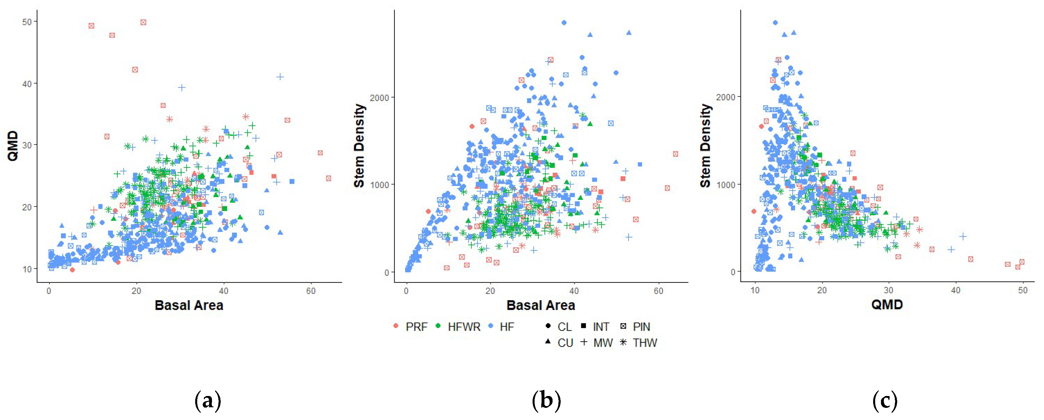
Forests 10 00226 g007
Table 1. Field data specifications.
ParameterPRFHFWR 1HF 2
Data collection2016, 2017
(June–July)
2008, 2010, 2011
(May–October)
2010
(June–July)
Number of plots84185387
Plot size (m2)10002500400
DBH threshold (cm)999
Species’ relative abundance (> 5%)E. white pine (29%)
White spruce (10%)
Balsam fir (9%)
Red maple (8%)
Red pine (8%)
Red oak (7%)
Sugar maple (29%)
Eastern hemlock (19%)
Red maple (11%)
American beech (9%)
Balsam fir (7%)
Yellow birch (7%)
Black spruce (37%)
Trembling aspen (14%)
Jack pine (11%)
White spruce (11%)
N. white cedar (9%)
Balsam fir (6%)
GPS unit
(listed accuracy)
SX Blue II-GNSS
(2drms = sub-60 cm, 95% confidence)
Trimble ProXT
(rms = 20–30 cm, in real time: sub-meter, 63% confidence)
SX Blue II-
GNSS
(2drms = sub-60 cm, 95% confidence)
PRF = Petawawa Research Forest; HFWR = Haliburton Forest and Wildlife Reserve; HF = Hearst Forest; 1 see Spriggs et al. [53], 2 see Penner et al. [13].
Table 2. Field data summaries (mean and standard deviation) for all sample plots and by provincial forest types.
FRI AttributeForest Type *
(n in Site Order)
PRF
(n = 84)
HFWR
(n = 185)
HF
(n = 387)
Basal Area (BA) All29.3/11.127.5/7.322.4/12.4
(m2 ha−1)CL (5, 0, 114)
CU (8, 22, 97)
16.3/8.3
28.0/5.7
-
34.2/8.5
21.3/10.8
21.3/13.5
INT (8, 12, 53)34.9/9.630.2/6.025.7/11.6
MW (9, 59, 62)26.6/8.030.1/6.927.0/9.9
PIN (39, 0, 61)31.1/12.7-18.4/14.4
THW (15, 92, 0)28.5/8.823.8/5.2-
Quadratic Mean All22.6/7.922.3/4.216.7/5.1
Diameter (QMD) (cm)CL (5, 0, 114)
CU (8, 22, 97)
15.5/4.8
20.3/4.5
-
22.2/4.1
14.5/2.4
15.5/3.8
INT (8, 12, 53)20.4/3.618.6/2.719.7/5.3
MW (9, 59, 62)18.3/2.423.6/5.121.6/6.0
PIN (39, 0, 61)25.1/9.4-15.3/4.8
THW (15, 92, 0)23.3/7.122.0/3.5-
Stem Density (S)All881/429757/3141019/573
(stems ha−1)CL (5, 0, 114)
CU (8, 22, 97)
898/454
942/348
-
925/320
1259/578
1036/603
INT (8, 12, 53)1074/1461131/238891/424
MW (9, 59, 62)1034/320757/312820/428
PIN (39, 0, 61)850/534-860/605
THW (15, 92, 0)731/255667/271-
* Forest type abbreviations: CL = conifers, lowland; CU = conifers, upland; INT = intolerant hardwoods (poplar and white birch); MW = mixedwoods; PIN = pines (white, red, and jack pine); THW = tolerant hardwoods.
Table 3. Airborne laser scanning (ALS) sensor specifications.
ParameterPRFHFWR 1HF 2
SensorTeledyne Titan Optech ALTM 3100Leica ALS50
Acquisition dateJuly 2016August 2009July-Sept. 2007
Wavelength (nm)1064 (channel 2)10641064
Pulse rate (kHz)37570119
Scan rate (Hz)403632
Scan half angle (°)201615
Flying height (km agl)1.11.52.4
Overlap (%)503020
Average pulse density [range] (ppm2)~ 12.4 [2.5–20.4]~ 2.5 [0.8–9.0]~ 1.5 [0.3–7.8]
1 see Spriggs et al. [53], 2 see Penner et al. [13].
Table 4. Site level BA, QMD, and S predictive RF model accuracies (%RMSE, %Bias, and R2, respectively) for the four different predictor sets (H only: normalized height metrics; H+T: normalized height and CHM texture metrics; H+I: normalized height and intensity metrics; and H+T+I: normalized height, CHM texture and intensity metrics) using leave-one-out cross-validation.
FRISiteH onlyH+TH+IH+T+I
RMSEBiasR2RMSEBiasR2RMSEBiasR2RMSEBiasR2
BAPRF22.8−0.110.6322.90.260.6321.70.200.6721.80.340.67
HFWR22.20.520.3121.30.230.3621.20.240.3720.80.400.40
HF25.40.360.7924.90.340.8025.30.380.7924.70.350.80
QMDPRF25.9−0.900.4526.3−0.520.4325.4−0.940.4725.5−0.700.46
HFWR12.30.190.5812.30.140.5811.80.270.6112.00.220.60
HF13.30.290.8112.90.270.8213.30.280.8112.90.290.82
S PRF41.40.980.2742.80.750.2238.01.260.4139.41.100.36
HFWR30.00.790.4828.00.430.5524.00.690.6724.00.530.67
HF30.80.600.7029.50.500.7330.20.600.7229.10.740.74
Best models in terms of %RMSE, %Bias or R2 are indicated in bold.
Table 5. Site level prediction error differences between the RF models with different predictor sets (H only: normalized height metrics; H+T: normalized height and CHM texture metrics; H+I: normalized height and intensity metrics; and H+T+I: normalized height, CHM texture and intensity metrics). p-values of the prediction error differences were acquired using the paired, nonparametric Friedman’s test.
FRISiteALS Dataset Differences
p-Value
PRF0.84
BA (m2 ha−1)HFWR0.23
HF0.42
PRF0.81
QMD (cm)HFWR0.40
HF0.65
PRF0.44
S (stems ha−1)HFWR0.44
HF0.34