Cross-Domain Bearing Fault Diagnosis Under Class Imbalance: A Dynamic Maximum Triple-View Classifier Discrepancy Network

Abstract

Traditional domain adaptation methods often assume balanced data distributions. However, this assumption is frequently violated in real-world industrial scenarios, where normal samples predominate while fault samples are inherently scarce. Under severe class imbalance, conventional decision boundaries tend to shift toward minority fault regions. This shift leads to persistently high misclassification rates for rare fault samples. To overcome this limitation, we propose the Dynamic Maximum Triple-View Classifier Discrepancy (DMTVCD) network, which integrates a Triple-View Classifier (TVC) Architecture and a Primary–Auxiliary Fused Cooperative Loss (PAFL). Specifically, the TVC employs auxiliary binary classifiers to aggregate fine-grained fault sub-classes into a unified “Fault Super-class.” This constructs a robust “normal-fault” binary boundary that effectively counteracts class imbalance. Driven by the PAFL, this boundary acts as a hierarchical geometric constraint to suppress the primary classifier’s tendency to misclassify faults as normal samples, thereby enhancing feature discriminability. Furthermore, a dynamic weighting strategy is introduced to assign large initial weights. This forces the model to bypass simple decision logic dominated by the majority class, ensuring a smooth transition from global exploration to fine-grained alignment. Extensive evaluations on the CWRU and JNU datasets demonstrate that DMTVCD consistently outperforms state-of-the-art approaches under high imbalance ratios (e.g., 20:1).

1. Introduction

Rolling bearings are core components of rotating machinery. Their health status is directly correlated with operational safety and production efficiency [1,2]. With the deep integration of the Industrial Internet of Things and artificial intelligence, data-driven deep learning methods have become the mainstream paradigm for fault diagnosis, owing to their powerful feature extraction capabilities [3].

Early research primarily focused on mining feature representations from massive supervised data. These methods rely on the idealized assumption that training data is abundant and identically distributed. Under such conditions, deep learning models demonstrate superior accuracy. For instance, Altaf et al. [4] fused statistical features with Support Vector Machines (SVM) for efficient state classification. To enhance discriminability, Yu et al. [5] proposed a Class-Level Autoencoder (CLAE) to enforce intra-class compactness. Zheng et al. [6] developed an adaptive group-sparse feature decomposition method to identify early faults in noisy environments. Similarly, Yu et al. [7] utilized a Multiscale Representations Fusion network to capture comprehensive signal patterns. Wang et al. [8] verified the advantages of Convolutional Neural Networks (CNN) in automatic feature extraction via time–frequency analysis.

However, supervised learning relies heavily on large amounts of manually annotated data. Furthermore, it requires the training and testing sets to follow the same probability distribution. In practical engineering scenarios, this requirement is often unmet. Operating conditions such as load and speed fluctuations cause shifts in data distributions, known as domain shift. Consequently, the generalization ability of traditional models faces severe challenges.

Domain Adaptation (DA) technology has emerged to address these challenges. DA aims to overcome distribution discrepancies by mining shared knowledge between labeled source domains and unlabeled target domains [9,10]. Representative works include the Deep Discriminative Transfer Learning Network (DDTLN) [11], which minimizes distributional distance in a Reproducing Kernel Hilbert Space. Deep Domain Confusion (DDC) [12] utilizes Maximum Mean Discrepancy (MMD) for feature alignment. Ganin et al. [13] introduced the Domain-Adversarial Neural Network (DANN), establishing the paradigm of adversarial distribution alignment. Furthermore, Maximum Classifier Discrepancy (MCD) [14] utilizes a game between classifiers and a generator to achieve success in cross-domain tasks.

To further exploit fine-grained structures, recent studies have explored deeper alignment strategies. For instance, Cross-domain Manifold Distance Adaptation (CMDA) [15] minimizes discrepancies in manifold space. DVSMN [16] leverages Graph Neural Networks to capture topological structures. Addressing data scarcity, Yang et al. [17] introduced a Cluster Contrastive Learning framework (CLCO) to extract domain-invariant features. To tackle severe domain shifts, Chen et al. [18] recently proposed a Triple Domain Adversarial Neural Network (TDANN). By integrating multiscale features with a triple-classifier architecture, TDANN aligns both marginal and conditional distributions while enhancing stability through an adaptive backpropagation coefficient.

Although these domain adaptation methods effectively mitigate distribution differences, most existing studies assume balanced category distributions. This overlooks the critical reality of class imbalance in industrial monitoring. Mechanical equipment operates in a healthy state for long periods, leading to a scarcity of fault data. Under the dual constraints of domain shift and class imbalance, conventional decision boundaries often bias toward the majority class (normal state). This bias results in severe missed detections of minority fault samples [19,20].

Methods such as Borderline-SMOTE [21], clustering-based undersampling [22], and Modified ACGAN [23] have made progress in addressing single imbalance issues. Recent frameworks, such as CVAE-SKEGAN combined with semi-supervised Swin Transformers [24], have also tackled compound challenges of imbalance and scarce labels. However, their direct application to cross-domain scenarios often fails because they cannot simultaneously account for domain feature alignment.

To resolve this dilemma, this paper proposes the Dynamic Maximum Triple-View Classifier Discrepancy (DMTVCD) network. The main contributions are as follows:

• We propose a Triple-View Classifier (TVC) Architecture based on a Sample Aggregation Mechanism and Primary–Auxiliary Fused Cooperative Loss (PAFL). To address minority sample scarcity, we introduce an auxiliary binary classification view. The Sample Aggregation Mechanism aggregates fine-grained fault sub-classes into a unified “Fault Super-class.” This fundamentally reduces the imbalance ratio and helps learn a robust “normal-fault” boundary. Driven by PAFL, this boundary acts as a hierarchical geometric constraint to suppress the primary classifier’s tendency to misclassify faults as normal. This explicitly prevents the decision boundary from encroaching upon minority regions, significantly reducing missed detections.
• We develop a dynamic weighting strategy to adaptively regulate the adversarial process. A dynamic factor is introduced to regulate the weight of the discrepancy loss. In the early training stage, a larger weight amplifies the divergence between classifiers. This forces the generator to conduct extensive feature exploration and prevents premature convergence to majority-class local optima. In the later stage, the weight is reduced to enforce consensus and promote compact alignment.
• We validate superior diagnostic robustness under extreme class imbalance. Extensive experiments on CWRU and JNU datasets confirm that even under an extreme 20:1 imbalance ratio, DMTVCD maintains superior performance, significantly outperforming state-of-the-art methods.

2. Related Work: Maximum Classifier Discrepancy (MCD)

Maximum Classifier Discrepancy (MCD) is a classic unsupervised domain adaptation method designed to align the distributions of source and target domains by leveraging task-specific decision boundaries. Unlike traditional approaches that attempt to directly match marginal distributions in the feature space, the core intuition of MCD is to utilize the prediction discrepancy between two classifiers to detect target domain samples that fall outside the support of the source domain.

2.1. Basic Architecture and Discrepancy Metric

As shown in Figure 1, the architecture of the MCD model comprises a feature generator G and two classifiers, $F_1$ and $F_2$, which share the same structure but are initialized differently. The generator G is responsible for mapping raw input data into a high-dimensional feature space, while the classifiers $F_1$ and $F_2$ are tasked with categorizing samples into K classes based on the extracted features.

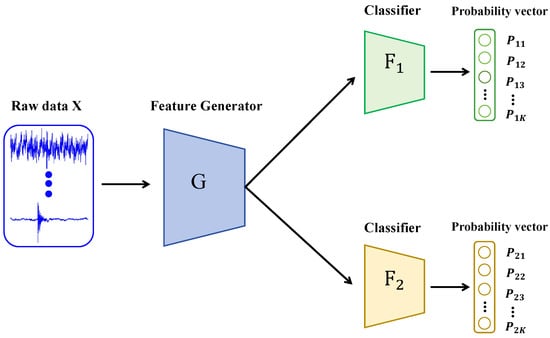
Figure 1. The schematic principle of the MCD method architecture.

To quantify the inconsistency in predictions between the two classifiers, the MCD method introduces a discrepancy loss. For a target domain sample $x_t$, this loss is typically defined as the L1 distance between the probability vectors output by the two classifiers:

$$d(p_1,p_2)={\displaystyle \frac{1}{K}}\sum _{j=1}^K|p_{1j}-p_{2j}|$$

(1)

where $p_{1j}$ and $p_{2j}$ denote the predicted probabilities of the j-th class by classifiers $F_1$ and $F_2$, respectively. A larger discrepancy value indicates a greater divergence in the judgments of the two classifiers regarding the sample, implying that the sample likely resides outside the source domain classification boundary or in a region with significant distribution shifts.

2.2. Adversarial Training Steps

MCD employs a minimax adversarial training strategy to optimize the generator and classifiers, prompting the generator to produce domain-invariant features capable of deceiving the classifiers (i.e., inducing consensus). The training process consists of the following three steps:

Step A: Source Domain Supervision. First, the generator G and the two classifiers $F_1,F_2$ are trained utilizing labeled source domain data $(X_s,Y_s)$. By minimizing the standard cross-entropy loss ${\mathcal{L}}_{cls}$, the model ensures fundamental classification capability on the source domain and enables the two classifiers to correctly partition source samples.

$$\underset{G,F_1,F_2}{min}{\mathcal{L}}_{cls}(X_s,Y_s)$$

(2)

Step B: Maximize Discrepancy. In this step, the parameters of the generator G are fixed, and only the two classifiers $F_1$ and $F_2$ are updated. The optimization objective is to maximize the discrepancy loss $d(p_1,p_2)$ on target domain samples $X_t$ while maintaining classification accuracy on the source domain. The purpose of this step is to force the two classifiers to diverge as much as possible in regions of the target domain feature space not covered by the source domain support (i.e., classification ambiguous regions), thereby identifying misaligned target samples.

$$\underset{F_1,F_2}{min}{\mathcal{L}}_{cls}(X_s,Y_s)-d(p_1\left(X_t\right),p_2\left(X_t\right))$$

(3)

Step C: Minimize Discrepancy. In this step, the parameters of the two classifiers $F_1$ and $F_2$ are fixed, and only the generator G is updated. The optimization objective is to minimize the discrepancy loss $d(p_1,p_2)$ on target domain samples. The aim is to compel the generator to produce features that facilitate agreement between the previously divergent classifiers, effectively pushing target domain samples into the interior of the source domain decision boundaries to achieve feature alignment.

$$\underset{G}{min}d(p_1\left(X_t\right),p_2\left(X_t\right))$$

(4)

By alternately executing Step B and Step C, the model synergistically optimizes the feature extractor and classifiers to learn deep feature representations that possess both class discriminability and domain invariance, thereby enabling effective cross-domain fault diagnosis. The schematic principle of the MCD method is presented in Figure 2.

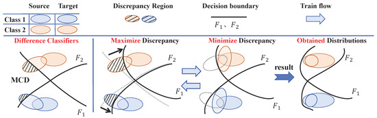
Figure 2. Visualization of training process with MCD method.

However, the standard MCD method implicitly operates under the assumption of balanced class distributions, a premise that sharply contrasts with the reality of industrial scenarios characterized by abundant normal samples and scarce fault samples. Under the dual constraints of domain shift and class imbalance, the optimization trajectory of the loss function is inevitably dominated by the majority class. Consequently, the decision boundary tends to encroach upon the minority class region (as illustrated by the comparison in Figure 3), biasing predictions toward the normal state. This boundary bias results in a high false-negative rate for fault samples. Addressing this limitation serves as the primary motivation for the improvements proposed in this paper.

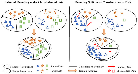
Figure 3. The effect of unbalanced data on trained classifier boundaries.

3. Proposed Method: DMTVCD

This section details the proposed Dynamic Maximum Triple-View Classifier Discrepancy (DMTVCD) network. The framework is designed to rectify decision boundary shifts caused by class imbalance under cross-domain conditions. It achieves this through a Triple-View Classifier (TVC) Architecture and a dynamic weighting strategy.

3.1. Problem Definition

Consider an unsupervised domain adaptation fault diagnosis scenario given a labeled source domain ${\mathcal{D}}_s={\left\{(x_i^s,y_i^s)\right\}}_{i=1}^{n_s}$ and an unlabeled target domain ${\mathcal{D}}_t={\left\{x_j^t\right\}}_{j=1}^{n_t}$. The label space consists of K classes, $y\in \{0,1,\dots ,K-1\}$, where class 0 represents the normal state and the remaining $K-1$ classes correspond to different fault types. Let $N_{normal}$ and $N_{fault}^{\left(k\right)}$ denote the number of samples in the normal class and the k-th fault class ($k\in \{1,\dots ,K-1\}$), respectively. In alignment with industrial reality, we assume severe inter-class imbalance in both domains, satisfying $N_{normal}\gg N_{fault}^{\left(k\right)}$. To quantify this disparity, the imbalance ratio is defined as $\rho =N_{normal}/N_{fault}^{\left(k\right)}$. The primary objective is to train a robust neural network for the target domain. This requires the model to simultaneously eliminate domain shift ($P_s\left(X\right)\ne P_t\left(X\right)$) and counteract the diagnostic bias induced by severe class imbalance.

3.2. DMTVCD Network Architecture

Framework Overview: To effectively rectify the decision boundary bias caused by domain shift and extreme class imbalance, we propose the DMTVCD framework. As illustrated in Figure 4, the overall architecture essentially consists of two core components: a 1D-CNN based Feature Generator (G) and a Triple-View Classifier (TVC) module. Specifically, the TVC integrates a fine-grained Primary Classifier ($C_{main}$) and two coarse-grained Auxiliary Classifiers ($C_{aux1},C_{aux2}$). The proposed framework is designed to facilitate a functional synergy: while $C_{main}$ is dedicated to the final K-class fault diagnosis, the auxiliary branches ($C_{aux1,2}$) serve exclusively as structural regularizers during the training phase. By aggregating fine-grained labels into a “Fault Super-class”, the auxiliary classifiers help in constructing a robust geometric decision boundary that prevents the primary decision boundary from shifting toward minority fault regions. Crucially, these auxiliary branches are discarded during inference, allowing the network to maintain high-precision diagnostic output with minimal computational overhead.

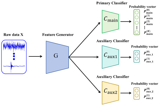
Figure 4. The proposed DMTVCD framework.

As illustrated in Figure 4, the detailed design of each component is formulated as follows:

• Feature Generator (G): Taking inspiration from the WDCNN architecture [25], we implement a deep 1-Dimensional Convolutional Neural Network (1D-CNN) as the feature extractor to achieve efficient end-to-end learning. Compared to traditional signal processing methods (e.g., FFT or Wavelet) which heavily rely on domain prior knowledge, or 2D-CNNs which introduce significant time–frequency conversion latency, our 1D-CNN directly extracts discriminative high-dimensional feature vectors from raw vibration signals. For source domain input $X_s$ and target domain input $X_t$, the extracted features are denoted as $f_s=G\left(X_s\right)$ and $f_t=G\left(X_t\right)$, respectively. Specifically, it utilizes a wide first-layer kernel ($16\times 1$) to effectively suppress high-frequency noise and capture the periodic impulsive characteristics inherent in bearing faults, followed by smaller kernels (e.g., $3\times 1$) for deep nonlinear mapping. This design provides a superior balance between feature discriminability and high computational efficiency required for real-time edge deployment.
• Triple-View Classifier (TVC) Architecture: To address the issue where multi-class classifiers tend to overlook minority classes under imbalanced data distributions, we design a synergistic module containing three independent classifiers:
  • Primary Classifier ($C_{main}$): A K-class multi-classifier outputting probabilities $p_{main}\left(X\right)\in {\mathbb{R}}^K$. Its task is to identify fine-grained specific health states.
  • Auxiliary Classifiers ($C_{aux1},C_{aux2}$): Two binary classifiers tasked with coarse-grained discrimination between normal and fault states. In our implementation, both auxiliary classifiers share an identical two-layer multi-layer perceptron (MLP) architecture. Specifically, this comprises a hidden layer with 256 units followed by a ReLU activation function, and a linear output layer yielding 2-dimensional predictions. To ensure they capture diverse discriminative features and establish a meaningful discrepancy space during adversarial training, $C_{aux1}$ and $C_{aux2}$ are independently initialized using Kaiming uniform initialization with different random seeds. This explicit structural design and independent initialization strategy firmly guarantee the constructing of a robust geometric decision boundary.

Sample Aggregation Mechanism: To facilitate the training of the auxiliary classifiers, we introduce a label-mapping function $\Phi$ to map the source domain K-class labels $Y_s$ to binary labels $Y_{s\_bin}$:

$$Y_{s\_bin}=\Phi \left(Y_s\right)=\left\{\begin{array}{cc}0,\hfill & \mathrm{if}{Y}_s=0\left(\mathrm{Normal}\right)\hfill \\ 1,\hfill & \mathrm{if}{Y}_s>0\left(\mathrm{Fault}\right)\hfill \end{array}\right.$$

(5)

For instance, taking the CWRU dataset as an example, the label space consists of $K=10$ classes, where label 0 denotes the normal state and labels 1 to 9 represent specific fine-grained fault types. The mapping function $\Phi$ acts as a thresholding mechanism that identically preserves the normal label (0) while strictly converting all specific fault indices (1–9) to 1. From a theoretical standpoint, this aggregation mechanism fundamentally reconstructs the marginal label distribution $P\left(Y_s\right)$ into a near-balanced binary space. By aggregating all subdivided fault sub-classes into a single “Fault Super-class”, it significantly diminishes the numerical disparity between the majority normal samples and the scarce specific fault samples. This enables the auxiliary classifiers to learn a robust geometric decision boundary, which subsequently imposes a hierarchical constraint on the main classifier.

3.3. Dynamic Discrepancy Loss and Optimization Objectives

To equilibrate exploration and alignment within the feature space during adversarial training, we define a multi-task classification loss, an inter-view discrepancy loss, and a dynamic weighting factor.

3.3.1. Multi-Task Classification Loss

To guarantee the discriminative capability of the model on the source domain, we utilize the source domain data $X_s$ and their corresponding labels to simultaneously minimize the multi-class loss of the primary view and the binary loss of the auxiliary views. The total classification loss and its constituent terms are formulated as follows:

$${\mathcal{L}}_{cls}(X_s,Y_s)={\mathcal{L}}_{CE}(C_{main}\left(G\left(X_s\right)\right),Y_s)+\sum _{i=1}^2{\mathcal{L}}_{CE}(C_{aux\_i}\left(G\left(X_s\right)\right),Y_{s\_bin})$$

(6)

$${\mathcal{L}}_{CE}(C_{main}\left(G\left(X_s\right)\right),Y_s)=-{\mathbb{E}}_{({\mathbf{x}}_s,y_s)\sim (X_s,Y_s)}\left[\sum _{k=0}^{K-1}{\mathbb{1}}_{[y_s=k]}log\left(p_{main}^{\left(k\right)}\left(G\left({\mathbf{x}}_s\right)\right)\right)\right]$$

(7)

$${\mathcal{L}}_{CE}(C_{aux\_i}\left(G\left(X_s\right)\right),Y_{s\_bin})=-{\mathbb{E}}_{({\mathbf{x}}_s,y_s)\sim (X_s,Y_s)}\left[\sum _{j=0}^1{\mathbb{1}}_{[\Phi \left(y_s\right)=j]}log\left(p_{aux\_i}^{\left(j\right)}\left(G\left({\mathbf{x}}_s\right)\right)\right)\right]$$

(8)

$p_{main}^{\left(k\right)}(·)$ represents the predicted probability of the main classifier for the k-th class, while $p_{aux\_i}^{\left(j\right)}(·)$ represents the predicted probability of the i-th auxiliary classifier for the j-th binary class. Here, ${\mathbb{1}}_{[·]}$ denotes the indicator function, which equals 1 if the condition within the brackets is satisfied and 0 otherwise. $\Phi \left(y_s\right)$ serves as the label-mapping function that converts the original category $y_s$ into a binary label (0 for Normal, 1 for Faults).

3.3.2. Primary–Auxiliary Fused Discrepancy Loss (PAFL)

The discrepancy loss serves as the core component of the proposed PAFL, designed to quantify the prediction divergence among different views on target domain samples $X_t$. Given the dimensional disparity between the primary classifier (K-dimensional, denoted as $p_{main}$) and the auxiliary classifiers (2-dimensional, denoted as $p_{aux}$), we first define a probability aggregation mapping $\mathcal{M}$. This mapping projects the output of the primary classifier into a binary space by aggregating all fine-grained fault sub-classes into a unified “Fault Super-class”:

$${\widehat{p}}_{main}\left(X_t\right)=\mathcal{M}\left(p_{main}\left(X_t\right)\right)=\left[p_{main}^{\left(0\right)}\left(X_t\right),\sum _{k=1}^{K-1}{p}_{main}^{\left(k\right)}\left(X_t\right)\right]$$

(9)

Here, ${\widehat{p}}_{main}$ represents the mapped binary probability vector, where the zeroth component corresponds to the normal class and the first component corresponds to the aggregated fault super-class. Based on this alignment, the discrepancy loss ${\mathcal{L}}_{disc}\left(X_t\right)$ is formulated as the average L1 distance over the binary categories, comprising two synergistic terms:

$${\mathcal{L}}_{disc}\left(X_t\right)=\underset{\mathrm{Hierarchical}\mathrm{Geometric}\mathrm{Constraint}\mathrm{Term}}{\underbrace{{\displaystyle \frac{1}{2}}\sum _{i=1}^2\sum _{j=0}^1\left|{\widehat{p}}_{main}^{\left(j\right)}\left(X_t\right)-p_{aux\_i}^{\left(j\right)}\left(X_t\right)\right|}}+\underset{\mathrm{Binary}\mathrm{Boundary}\mathrm{Reinforcement}\mathrm{Term}}{\underbrace{{\displaystyle \frac{1}{2}}\sum _{j=0}^1\left|p_{aux\_1}^{\left(j\right)}\left(X_t\right)-p_{aux\_2}^{\left(j\right)}\left(X_t\right)\right|}}$$

(10)

where $j\in \{0,1\}$ denotes the binary class index. This formulation embodies a dual-role scheme:

• The Hierarchical Geometric Constraint Term (first part) acts as a hard constraint enforced by the auxiliary views. Geometrically, the robust “normal-fault” decision boundary established by the auxiliary classifiers acts as an anchor. It compels the primary classifier to align its aggregated predictions with the robust binary boundary, effectively suppressing the tendency of the primary decision boundary to shift towards and misclassify fault samples as normal under extreme class imbalance.
• The Binary Boundary Reinforcement Term (second part) maximizes the discrepancy between the two auxiliary views. This explicitly mines ambiguous samples at the coarse-grained level to construct a robust “normal-fault” geometric boundary.

3.3.3. Dynamic Weighting Factor

Ganin et al. [13] established within the Domain-Adversarial Neural Network (DANN) framework that the adaptive modulation of adversarial weights is pivotal for ensuring training stability during domain adaptation. Drawing inspiration from this insight, and to overcome the limitation where static weights fail to reconcile the conflicting requirements of initial feature exploration and subsequent model convergence, this paper develops a reverse exponential decay strategy. Accordingly, a dynamic weighting factor $\omega \left(t\right)$ is proposed, which is defined as a function that exhibits exponential decay relative to the training epoch t:

$$\omega \left(t\right)={\lambda }_0·exp\left(-\mu ·{\displaystyle \frac{t}{T_{max}}}\right)$$

(11)

where t denotes the current training epoch, and $T_{max}$ represents the preset total number of epochs. ${\lambda }_0$ is the initial weight, ensuring that extremely high attention is assigned to the discrepancy loss in the initial stage to maximize classifier divergence. This compels the classifiers to engage in global feature exploration and explicitly forces the generator to break away from simple decision logic dominated by the majority class. $\mu$ is the decay rate coefficient, which controls the transition speed from exploration to convergence. As training proceeds, $\omega \left(t\right)$ decays smoothly, gradually shifting the model’s focus toward fine-grained feature alignment and ensuring that the classifiers reach a highly consistent decision by the end of training.In our network implementation, we empirically set the initial weight ${\lambda }_0=2.0$, the decay rate $\mu =0.5$, and the total training epochs $T_{max}=100$. Under these settings, the dynamic weighting factor $\omega \left(t\right)$ starts at a peak value of $2.0$ at epoch 0, enforcing aggressive discrepancy maximization to thoroughly explore the target domain feature space. By the middle of the training phase (e.g., $t=50$), $\omega \left(t\right)$ smoothly decays to approximately $1.56$, gradually relaxing the adversarial penalty. Towards the final epochs ($t=100$), it decays to $1.21$. This continuous decay mechanism effectively prevents the severe optimization oscillations and non-convergence issues that frequently occur when using a persistently high static weight, thereby allowing the model to smoothly transition its focus toward structural feature preservation and stable fine-grained alignment.

3.4. Adversarial Training Steps

DMTVCD employs an improved Min-Max game strategy. In each training batch, the network parameters are updated alternately using source domain data $X_s$ and target domain data $X_t$ according to the following three steps:

Step A: Source Domain Supervision. Update the generator G and all classifiers C to minimize the total classification loss on the source domain. This step aims to establish preliminary decision boundaries, endowing the model with fundamental classification discrimination capabilities. The objective is as follows:

$$\underset{G,C}{min}{\mathcal{L}}_{cls}(X_s,Y_s)$$

(12)

Step B: Maximizing Discrepancy to Drive Global Exploration. Fix the generator G and update all classifiers C to maximize the discrepancy loss on the target domain while maintaining source domain classification accuracy. The objective is as follows:

$$\underset{C}{min}{\mathcal{L}}_{cls}(X_s,Y_s)-\omega \left(t\right)·{\mathcal{L}}_{disc}\left(X_t\right)$$

(13)

Step Description: In this step, $\omega \left(t\right)$ controls the intensity of the adversarial process. In the initial stage, a large $\omega \left(t\right)$ makes the discrepancy term dominate the loss function, forcing the classifiers to engage in global feature exploration in the target domain feature space. Crucially, this high-intensity adversity forces the model to break away from simple decision logic dominated by the majority class by exposing ambiguous samples near the decision boundaries. As $\omega \left(t\right)$ decays, the optimization objective gradually shifts focus toward preserving feature structure, preparing for refined alignment.

Step C: Minimizing Discrepancy to Facilitate Domain Alignment. Fix all classifiers C and update the generator G to minimize the discrepancy loss. The objective is as follows:

$$\underset{G}{min}{\mathcal{L}}_{disc}\left(X_t\right)$$

(14)

Step Description: In this step, the generator strives to generate features that can simultaneously deceive the main and auxiliary classifiers (i.e., reducing prediction discrepancy).

By alternately executing Step B and Step C for n times, where n is defined as a model training hyperparameter, the model achieves a dynamic balance between vigorous correction in the early stage and stable alignment in the later stage. This process ultimately generates robust feature representations that possess both class discriminability and domain invariance, thereby realizing effective cross-domain fault diagnosis. The specific procedure is outlined in Algorithm 1.

Algorithm 1 Training procedure of DMTVCD.

Require: Source domain ${\mathcal{D}}_s$, Target domain ${\mathcal{D}}_t$; Batch size m, Epochs $T_{max}$, Steps n; Params ${\lambda }_0,\mu ,\eta$. Ensure: Optimized parameters ${\theta }_G,{\theta }_C$.    1: Initialize parameters ${\theta }_G$ and ${\theta }_C$ ($C_{main},C_{aux1},C_{aux2}$).    2: for $t=1$ to $T_{max}$ do    3:    Calculate dynamic weighting factor: $\omega \left(t\right)={\lambda }_0·exp\left(-\mu ·{\displaystyle \frac{t}{T_{max}}}\right)$.    4:    for each mini-batch $(X_s,Y_s)$ from ${\mathcal{D}}_s$ and $X_t$ from ${\mathcal{D}}_t$ do      5:       Step A: Source Domain Supervision    6:       Construct binary labels: $Y_{s\_bin}=\Phi \left(Y_s\right)$.    7:       Update parameters ${\theta }_G,{\theta }_C$ by optimizing:    8:          ${\displaystyle \underset{G,C}{min}{\mathcal{L}}_{cls}(X_s,Y_s)}$      9:       // Adversarial Training Loop  10:       for $k=1$ to n do  11:          Step B: Maximize Discrepancy  12:          Fix ${\theta }_G$, update ${\theta }_C$ by optimizing:  13:             ${\displaystyle \underset{C}{min}({\mathcal{L}}_{cls}(X_s,Y_s)-\omega \left(t\right)·{\mathcal{L}}_{disc}\left(X_t\right))}$  14:          Step C: Minimize Discrepancy  15:          Fix ${\theta }_C$, update ${\theta }_G$ by optimizing:  16:             ${\displaystyle \underset{G}{min}\left({\mathcal{L}}_{disc}\left(X_t\right)\right)}$  17:       end for  18:    end for  19: end for

4. Experimental Verification

We conducted experiments on the Case Western Reserve University (CWRU) and Jiangnan University (JNU) bearing datasets to evaluate the effectiveness and superiority of the proposed DMTVCD method in cross-domain fault diagnosis under class imbalance and varying operating conditions. Furthermore, ablation studies were performed to further verify the effectiveness of the dynamic weighting strategy.

4.1. Dataset Description and Imbalanced Sample Construction

4.1.1. CWRU Bearing Dataset

The CWRU bearing dataset is recognized as one of the most classic open-source datasets in the field of mechanical fault diagnosis. It was collected by Case Western Reserve University using a motor test rig [26]. In this experiment, drive-end accelerometer data sampled at 12 kHz was selected. The experiments simulated four distinct load conditions: 0, 1, 2, and 3 hp (corresponding to rotational speeds of 1797 r/min, 1772 r/min, 1750 r/min, and 1730 r/min, respectively). The data comprises 10 health state categories: 1 normal state (Normal) and 3 fault types (Inner Race Fault, Outer Race Fault, Rolling Element Fault), with each fault type containing three different damage diameters (0.007 mil, 0.014 mil, and 0.021 mil). To simulate cross-domain diagnosis under variable operating conditions, data collected under different loads were defined as distinct domains. For instance, the task “0 hp→1 hp” denotes that the source domain is 0 hp data and the target domain is 1 hp data. Following Z-score normalization preprocessing, each health state category under each condition contains 500 samples with a length of 1024.

4.1.2. JNU Bearing Dataset

The JNU bearing dataset was provided by the Institute of Intelligent Fault Diagnosis at Jiangnan University [27]. Collected from a centrifugal fan test rig designed to simulate industrial field environments, this dataset contains more significant background noise and mechanical vibration interference compared to the CWRU dataset. Therefore, it is widely used to verify the robustness of algorithms under complex noisy environments and varying speed conditions. Experimental data were collected under three speed conditions: 600 r/min, 800 r/min, and 1000 r/min. The data includes 4 health states: Normal, Inner Race Fault (IF), Outer Race Fault (OF), and Rolling Element Fault (RF). Different speed conditions were set as distinct domains to construct cross-speed transfer tasks. After Z-score normalization preprocessing, each health state category under each condition contains 1000 samples with a length of 1024.

4.1.3. Imbalanced Sample Construction and Splitting

To faithfully simulate the extreme distribution characteristics of actual industrial scenarios where normal samples are massive but fault samples are scarce, we constructed training sets for both source and target domains based on the previously defined imbalance ratio. Specifically, the ratio of the number of normal samples to that of each individual fault category was set to $\rho =N_{normal}$:$N_{fault}^{\left(k\right)}$ = 20:1 for all experiments. The specific data splitting details are presented in Table 1 and Table 2.

Table 1. Data splitting for the CWRU dataset (Imbalance ratio $\rho$ = 20:1).

Health Condition	Training Source (Samples)	Training Target (Samples)	Testing Target (Samples)	Label
Normal	400	400	100	0
Inner Race (0.007″)	20	20	100	1
Inner Race (0.014″)	20	20	100	2
Inner Race (0.021″)	20	20	100	3
Ball (0.007″)	20	20	100	4
Ball (0.014″)	20	20	100	5
Ball (0.021″)	20	20	100	6
Outer Race (0.007″)	20	20	100	7
Outer Race (0.014″)	20	20	100	8
Outer Race (0.021″)	20	20	100	9

Table 2. Data splitting for the JNU dataset (Imbalance ratio $\rho$ = 20:1).

Health Condition	Training Source (Samples)	Training Target (Samples)	Testing Target (Samples)	Label
Normal	400	400	100	0
Inner Race Fault	20	20	100	1
Rolling Element Fault	20	20	100	2
Outer Race Fault	20	20	100	3

4.2. Comparison Methods and Parameter Configuration

4.2.1. Comparison Methods

To comprehensively verify the superiority of DMTVCD under extreme class imbalance conditions ($\rho =20$), five representative methods were selected for comparative analysis. These include: the Baseline CNN [25] trained only on the source domain, serving as a performance lower bound. Classic adversarial domain adaptation methods DANN [13] and MCD [14], and advanced methods recently proposed for complex cross-domain or imbalanced diagnosis tasks, namely CMDA [15] and DVSMN [16]. Notably, to ensure fair comparison, all the aforementioned transfer learning methods integrate a feature extractor architecture identical to that of the Baseline CNN.

4.2.2. Parameter Configuration

All model construction and training processes in this experiment were implemented within the PyTorch (version 1.10.2) framework using Python 3.6, utilizing a hardware platform equipped with an Intel Core i9-12900K CPU and an NVIDIA GeForce RTX 3090 GPU. Regarding network architecture, the feature generator G uniformly adopts a 5-layer one-dimensional Convolutional Neural Network (1D-CNN) to extract time–frequency features, while both the main classifier $C_{main}$ and the auxiliary classifier $C_{aux}$ are composed of two-layer fully connected networks. The specific network-layer structural parameters are presented in Table 3. Regarding the training strategy, the Adam optimizer is employed for parameter updates, with momentum parameters set to standard values of ${\beta }_1=0.9,{\beta }_2=0.999$, and the initial learning rate $\eta$ set to 0.001. Considering the scale of the experimental samples, to balance training stability and convergence speed, the batch size was set to 64, and the total number of training epochs is set to $T_{max}=100$. Furthermore, regarding the unique hyperparameters of the DMTVCD method, through optimization experiments, the initial discrepancy weight ${\lambda }_0$ was determined to be 2, the exponential decay rate $\mu$ was set to 0.5, and the alternating execution steps n were set to 6, so as to ensure optimal domain adaptation performance.

Table 3. Specific network-layer structural parameters of DMTVCD.

Module	Layer	Type	Configuration ($\mathit{k},\mathit{s},\mathit{p}$)	Output Shape
Feature Generator (G)	1	Conv1d + BN + ReLU MaxPool1d	$16\times 1,8,4$ $2\times 1,2,0$	$16\times 128$ $16\times 64$
	2	Conv1d + BN + ReLU MaxPool1d	$3\times 1,1,1$ $2\times 1,2,0$	$32\times 64$ $32\times 32$
	3	Conv1d + BN + ReLU MaxPool1d	$3\times 1,1,1$ $2\times 1,2,0$	$64\times 32$ $64\times 16$
	4	Conv1d + BN + ReLU MaxPool1d	$3\times 1,1,1$ $2\times 1,2,0$	$64\times 16$ $64\times 8$
	5	Conv1d + BN + ReLU MaxPool1d	$3\times 1,1,1$ $2\times 1,2,0$	$64\times 8$ $64\times 4$
Flatten Layer				256
Main Classifier ($C_{main}$)	1	Linear + ReLU	-	256
	2	Linear	-	K
Auxiliary Classifiers ($C_{aux1,2}$)	1	Linear + ReLU	-	256
	2	Linear	-	2

k: Kernel Size, s: Stride, p: Padding. K: Number of classes. Input size: 1 × 1024.

4.3. Analysis of Experimental Results on CWRU Dataset

Table 4 details the diagnostic accuracy and computation time on the CWRU dataset across 12 cross-load transfer tasks under the severe setting of a class imbalance ratio $\rho =20$. Experimental results indicate that the proposed DMTVCD method achieves state-of-the-art performance in all transfer tasks, yielding an impressive average accuracy of 95.81%, which represents a qualitative leap compared to the 72.79% accuracy of the source-only CNN baseline. Although mainstream methods such as MCD and CMDA reached average accuracies of 89.54% and 88.59%, respectively, they still exhibit limitations when confronting extreme class imbalance. Specifically, in the 3-0 task characterized by a large span of operating conditions, the accuracy of all comparative methods failed to exceed 84%, with the best-performing competitor CMDA reaching only 83.52%, whereas DMTVCD robustly maintained a high accuracy of 87.88%. Regarding computational efficiency, the average training time for DMTVCD is 37.0 s, which is slightly higher than the 35.2 s required by MCD. This is primarily attributed to the introduction of the Triple-View Classifier (TVC) Architecture and the requirement to alternatingly execute Step B and Step C for n iterations during the adversarial training phase to ensure decision boundary convergence. Although this mechanism leads to a marginal increase in computational cost, the trade-off is well justified in practical applications considering the significant gain in diagnostic accuracy.

Table 4. Diagnostic accuracy (%) and computation time (seconds) on the CWRU dataset across 12 cross-load tasks.

Task	CNN [25]		DANN [13]		MCD [14]		DVSMN [16]		CMDA [15]		DMTVCD
	Acc (%)	Time (s)	Acc (%)	Time (s)	Acc (%)	Time (s)	Acc (%)	Time (s)	Acc (%)	Time (s)	Acc (%)	Time (s)
0-1	69.66 ± 3.85	6.8	86.90 ± 4.88	8.5	89.90 ± 1.46	35.2	76.22 ± 2.86	13.4	86.12 ± 4.39	9.5	90.36 ± 4.85	39.5
0-2	69.84 ± 3.87	5.7	89.86 ± 3.20	12.5	90.18 ± 0.99	41.2	76.12 ± 1.23	18.5	91.88 ± 3.65	10.8	99.40 ± 0.28	40.7
0-3	65.62 ± 2.17	5.1	83.02 ± 5.66	4.6	90.52 ± 5.71	33.0	69.46 ± 2.44	10.5	89.84 ± 3.72	7.5	94.62 ± 7.03	38.9
1-0	76.68 ± 2.26	6.8	86.64 ± 2.43	9.3	89.66 ± 2.33	31.7	78.18 ± 4.13	13.3	84.02 ± 3.99	9.6	96.08 ± 1.58	25.1
1-2	79.18 ± 4.40	5.4	79.28 ± 4.00	13.0	93.40 ± 3.41	40.4	85.12 ± 3.41	17.0	90.86 ± 5.67	8.6	99.30 ± 0.77	45.5
1-3	70.92 ± 5.05	9.4	73.14 ± 3.21	14.0	89.96 ± 5.56	41.6	75.78 ± 3.83	9.6	87.98 ± 3.77	9.7	99.36 ± 0.45	41.9
2-0	75.78 ± 3.01	9.4	85.18 ± 2.35	12.2	86.78 ± 3.15	38.7	75.04 ± 4.14	11.5	84.10 ± 4.20	5.0	95.54 ± 0.94	31.0
2-1	77.58 ± 2.66	3.5	79.78 ± 2.35	4.6	92.50 ± 2.67	30.4	82.20 ± 2.76	10.4	88.92 ± 3.00	14.2	97.92 ± 1.06	39.0
2-3	77.78 ± 3.91	8.4	82.30 ± 3.17	10.7	96.98 ± 3.15	34.1	86.44 ± 3.04	6.7	96.40 ± 1.45	5.9	99.44 ± 0.28	37.2
3-0	67.22 ± 3.76	4.3	74.88 ± 4.02	10.4	79.78 ± 4.17	40.0	69.60 ± 4.81	16.0	83.52 ± 3.69	15.0	87.88 ± 5.40	38.4
3-1	67.98 ± 3.02	7.7	69.52 ± 2.08	6.1	81.62 ± 4.21	28.4	75.30 ± 4.05	13.9	84.10 ± 2.42	5.2	89.98 ± 4.95	27.8
3-2	75.26 ± 4.24	7.9	81.30 ± 3.07	7.4	93.14 ± 3.71	28.2	83.70 ± 3.44	14.8	95.30 ± 1.95	14.1	99.88 ± 0.07	39.5
Average	72.79	6.7	80.98	9.4	89.54	35.2	77.76	13.0	88.59	9.6	95.81	37.0

Furthermore, regarding deployment-related metrics, the proposed DMTVCD does not introduce any additional computational overhead during the inference phase compared to the standard CNN baseline. Although the Triple-View Classifier (TVC) Architecture slightly increases the training parameter count to 0.23 M and the peak memory footprint to 25.02 MB, the two auxiliary classifiers ($C_{aux1}$ and $C_{aux2}$) are utilized exclusively during the adversarial training phase. During actual industrial deployment and real-time inference, these auxiliary branches are completely discarded. Consequently, the deployed model consists solely of the feature generator G and the primary classifier $C_{main}$. The deployable parameter count is drastically reduced to 0.10 M, and the inference memory footprint drops to 19.06 MB. Furthermore, the inference latency for processing a single 1024-length vibration sample is merely 0.51 ms. This quantitatively demonstrates the lightweight deployment efficiency of DMTVCD, satisfying the strict requirements of high-frequency real-time condition monitoring on resource-constrained industrial edge devices. In summary, DMTVCD effectively mitigates the dual interference of class imbalance and domain shift through its unique synergistic design, demonstrating superior adaptability and robustness in complex cross-domain scenarios.

4.4. Analysis of Experimental Results on JNU Dataset

The diagnostic accuracy and computation time for the JNU dataset across 6 cross-speed transfer tasks, configured with a severe class imbalance ratio of $\rho =20$, are summarized in Table 5. Experimental results demonstrate that the proposed DMTVCD method delivers superior diagnostic performance even under complex noisy environments and varying speed conditions, achieving an average accuracy of 79.00%. Specifically, DMTVCD realizes significant performance improvements of 18.39% and 5.25% compared to the baseline CNN (60.61%) and the advanced CMDA method (73.75%), respectively. It is worth noting that while the MCD method performs well in certain tasks, reaching an average accuracy of 77.01%, its accuracy drops noticeably to 65.33% in the most challenging task 0-2, which involves large-span speed fluctuations, due to drastic shifts in domain distribution. In contrast, DMTVCD robustly maintains an accuracy of 71.47%, representing a 6.14% improvement over MCD. Regarding computational efficiency, the average training time for DMTVCD is 69.8 s, which is comparable to the 69.2 s required by MCD. This is similarly attributed to the introduction of the Triple-View Classifier (TVC) Architecture and the requirement to alternatingly execute Step B and Step C for n iterations during the adversarial training phase to optimize the decision boundary. Although this mechanism results in higher computational costs compared to lightweight methods like DANN, the investment is necessary given the enhanced robustness achieved against the dual interference of complex noise and class imbalance. In summary, DMTVCD effectively mitigates the adverse effects of noise on feature alignment through its unique synergistic design, demonstrating adaptability superior to existing methods under non-stationary operating conditions.

Table 5. Diagnostic accuracy (%) and computation time (seconds) on the JNU dataset across 6 cross-speed tasks.

Task	CNN [25]		DANN [13]		MCD [14]		DVSMN [16]		CMDA [15]		DMTVCD
	Acc (%)	Time (s)	Acc (%)	Time (s)	Acc (%)	Time (s)	Acc (%)	Time (s)	Acc (%)	Time (s)	Acc (%)	Time (s)
0-1	63.23 ± 2.80	8.9	70.12 ± 3.50	6.4	73.45 ± 5.69	55.0	65.72 ± 2.12	17.8	74.78 ± 3.84	11.6	80.58 ± 2.20	86.8
0-2	56.67 ± 3.67	8.1	64.10 ± 4.12	14.5	65.33 ± 6.08	73.6	58.17 ± 2.81	19.2	67.97 ± 4.41	16.1	71.47 ± 2.88	59.4
1-0	64.05 ± 2.67	8.1	73.45 ± 2.84	17.8	81.58 ± 1.06	75.0	68.33 ± 2.38	19.3	75.67 ± 3.86	17.0	79.42 ± 2.59	69.6
1-2	62.65 ± 5.24	4.1	71.35 ± 6.07	13.8	80.35 ± 4.40	78.8	66.17 ± 5.47	12.7	74.12 ± 5.23	14.6	83.22 ± 1.75	61.0
2-0	56.12 ± 3.39	7.5	67.10 ± 1.73	14.6	75.80 ± 2.97	63.5	58.85 ± 4.90	18.2	73.20 ± 3.05	16.4	76.20 ± 2.89	74.9
2-1	60.92 ± 4.45	8.8	73.45 ± 3.18	10.3	85.53 ± 3.12	68.9	64.80 ± 5.04	17.7	76.75 ± 4.21	12.6	83.12 ± 3.47	67.1
Average	60.61	7.6	69.93	12.9	77.01	69.2	63.67	17.5	73.75	14.7	79.00	69.8

4.5. Robustness to Varying Imbalance Ratios

To comprehensively evaluate the robustness of the proposed DMTVCD method under different degrees of data scarcity, we extended our experiments to include varying imbalance ratios: $\rho \in \{5,10,20,50\}$. We selected two representative cross-load tasks from the CWRU dataset: Task 3-0 (representing large domain shift) and Task 3-2 (representing small domain shift). The performance trends of DMTVCD and other comparative methods across these ratios are illustrated in Figure 5.

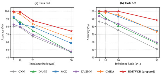
Figure 5. Performance trends of different methods under varying imbalance ratios on the CWRU dataset: (a) Task 3-0 and (b) Task 3-2.

As shown in Figure 5a, Task 3-0 is highly challenging. When the imbalance ratio escalates to an extreme 50:1, baseline methods suffer a drastic collapse in accuracy due to severe decision boundary bias towards the majority class (e.g., DANN and CNN plummet to 46.82% and 46.72%, respectively). In contrast, DMTVCD maintains a highly competitive accuracy of 74.22%, outperforming the second-best method (CMDA at 64.74%) by nearly 10%. Similarly, for the relatively easier Task 3-2 shown in Figure 5b, all methods perform well under mild imbalance ($\rho =5$). However, at $\rho =50$, traditional adversarial methods experience noticeable performance drops (e.g., MCD drops to 74.58%). DMTVCD, on the other hand, exhibits exceptional stability, sustaining a high accuracy of 88.38%. This quantitatively demonstrates that the hierarchical geometric constraint imposed by the “Fault Super-class” effectively anchors the decision boundary, ensuring strong diagnostic robustness over a wide, practical range of class imbalances.

4.6. Robustness in Complex and Strong-Noise Environments

To further validate the model’s adaptability in strong-noise industrial environments, we simulated a rigorous “Clean-to-Noisy” cross-domain scenario on the highly challenging Task 3-0 of the CWRU dataset. The source domain was kept pure, while two types of synthetic noise were strictly injected into the target domain data:

• Additive White Gaussian Noise (AWGN): Evaluated at specific Signal-to-Noise Ratios (SNRs: 8, 4, 0, and −4 dB) [28].
• Non-Gaussian Impulsive Interference: Simulating electromagnetic shocks and sensor packet loss via an occurrence probability $p\in \{0.01,0.03,0.05,0.10\}$. Affected data points were randomly replaced by either an extreme spike ($\pm 5A_{max}$, where $A_{max}$ is the maximum amplitude) or forced to 0 [17,29].

As illustrated in Figure 6, DMTVCD demonstrates exceptional robustness. Under AWGN (Figure 6a), even when noise completely overwhelms the signal (−4 dB), DMTVCD achieves 44.18% accuracy, significantly outperforming CMDA (23.24%). Under impulsive interference (Figure 6b), DMTVCD maintains high accuracies of 82.36% and 66.22% at practical probabilities of $p=0.01$ and $p=0.03$, respectively, surpassing the classic MCD method (68.62% and 53.50%) by a large margin. This confirms that the hierarchical constraints provided by the “Fault Super-class” effectively anchor decision boundaries against severe Gaussian and non-Gaussian perturbations.

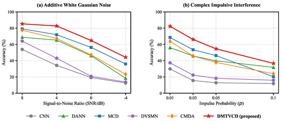
Figure 6. Performance comparison under varying complex noises on the CWRU dataset for Task 3-0: (a) Additive White Gaussian Noise (AWGN); (b) Non-Gaussian Impulsive Interference.

4.7. Ablation Study and Training Dynamics Analysis

To verify the critical role of the proposed dynamic weighting strategy in balancing feature exploration and domain alignment, an ablation study was conducted. A variant model, denoted as DMTVCD-Static, was constructed by fixing the adversarial weighting factor to a constant $\omega =1$, thereby maintaining a constant adversarial intensity throughout the training process.

The quantitative results are presented in Table 6. Although the static variant performs acceptably on certain simple tasks, its average accuracy is limited to 93.13%, representing a performance degradation of 2.68% compared to the complete DMTVCD method. This disparity is particularly pronounced in difficult tasks involving large operating condition shifts. Taking task 3-0 as an instance, the accuracy of DMTVCD-Static drops sharply to 78.60% due to the absence of a weight decay mechanism in the later stages, whereas the complete method maintains a high precision of 87.88%, reflecting a performance gap exceeding 9%.

Table 6. Ablation study results comparing DMTVCD with DMTVCD-Static ($\omega =1$) on the CWRU dataset.

Task	DMTVCD-Static ($\mathit{\omega }=1$)	DMTVCD (Dynamic $\mathit{\omega }$)
0-1	92.66 ± 1.72	90.36 ± 4.85
0-2	96.20 ± 1.12	99.40 ± 0.28
0-3	98.86 ± 0.41	94.62 ± 7.03
1-0	93.08 ± 1.90	96.08 ± 1.58
1-2	97.10 ± 1.15	99.30 ± 0.77
1-3	95.60 ± 3.31	99.36 ± 0.45
2-0	91.24 ± 2.49	95.54 ± 0.94
2-1	94.14 ± 1.68	97.92 ± 1.06
2-3	99.52 ± 0.20	99.44 ± 0.28
3-0	78.60 ± 2.96	87.88 ± 5.40
3-1	83.86 ± 3.27	89.98 ± 4.95
3-2	96.68 ± 2.38	99.88 ± 0.07
Average	93.13	95.81

To visually unpack the underlying optimization mechanism behind this performance gap and demonstrate the convergence behavior, we further recorded the training dynamics of key metrics on Task 3-0, as plotted in Figure 7. To clearly visualize the L1-norm based discrepancy loss alongside the larger cross-entropy loss within the same coordinate system, ${\mathcal{L}}_{disc}$ is scaled by a factor of 10.

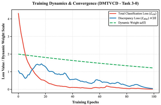
Figure 7. Training dynamics and convergence behavior of the proposed DMTVCD on Task 3-0.

The convergence dynamics perfectly corroborate our ablation findings, demonstrating a classic “exploration to consensus” adversarial process. During the early exploration phase (e.g., the first 40 epochs), the high initial value of $\omega \left(t\right)$ enforces a stringent adversarial penalty. This forces the discrepancy loss to maintain observable fluctuations and relatively high values (the visible “bumps” in the blue curve), effectively compelling the feature generator to break away from local, source-biased minima to rigorously explore the target domain space.

As training progresses and $\omega \left(t\right)$ smoothly decays, the severe min-max game oscillations are successfully mitigated. In the later alignment phase, both the classification loss and the discrepancy loss converge stably towards near-zero. In the MCD paradigm, a near-zero discrepancy loss signifies that the generator has successfully aligned the target features into the source distribution, compelling the independent classifiers to reach a complete “consensus”. This empirical dynamic analysis powerfully verifies that the dynamic weighting strategy successfully reconciles early-stage minority class mining with late-stage stable alignment, preventing the structural disruption typically caused by persistently high static weights.

4.8. Visualization Analysis

To intuitively evaluate the discriminative capability and domain adaptation effectiveness of the models in the feature space, the t-SNE technique was employed to visualize the high-dimensional features of the CWRU 0 HP → 3 HP task in a two-dimensional map. Figure 8 illustrates the spatial distribution of the raw signal data and the features extracted by the six comparative models. Observations reveal that both raw data and CNN features (Figure 8a,b) exhibit severe class overlap with indistinct boundaries, highlighting the distribution misalignment caused by domain shift in the absence of transfer strategies. Similarly, DVSMN (Figure 8c) displays significant overlap; this is likely because the standardization of the backbone to a 1D-CNN for fair comparison restricted its capacity to capture topological features. While DANN, CMDA, and MCD (Figure 8d–f) improve clustering structure to some extent, they still suffer from loose intra-class distributions and adhesion between certain fault categories. In contrast, the proposed DMTVCD method (Figure 8g) demonstrates the superior performance. All ten health state categories form well-defined and highly compact independent clusters, exhibiting exceptional intra-class compactness and inter-class separability. Even samples with varying damage severities within the same fault type, which share high feature similarity, are effectively mapped to distinct, non-overlapping regions. These visualization results provide compelling evidence that, under the synergistic action of triple-view constraints and the dynamic weighting strategy, DMTVCD effectively mitigates the interference of large-span domain shifts and class imbalance, extracting domain-invariant feature representations characterized by strong discriminability and robustness.

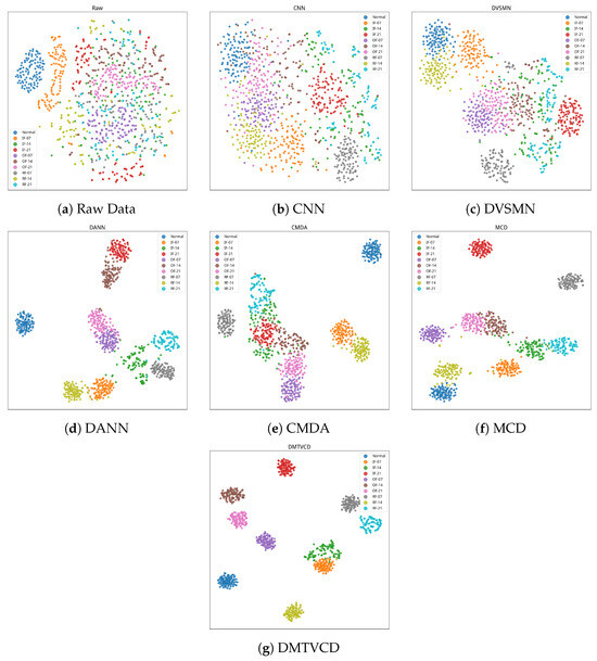
Figure 8. The t-SNE visualization of feature distributions: (a) Raw Data, (b) CNN, (c) DVSMN, (d) DANN, (e) CMDA, (f) MCD, (g) DMTVCD.

5. Conclusions

This paper proposes the Dynamic Maximum Triple-View Classifier Discrepancy (DMTVCD) network to address the dual challenges of domain shift and severe class imbalance, which are prevalent in rotating machinery. By leveraging the Triple-View Classifier (TVC) Architecture, the proposed method innovatively aggregates fine-grained faults into a unified “Fault Super-class” to construct a robust binary boundary. Acting as a hierarchical geometric constraint enforced by the Primary–Auxiliary Fused Cooperative Loss (PAFL), this mechanism effectively corrects the geometric distortion where decision boundaries shift toward the minority class region under imbalanced data distributions. Furthermore, by integrating an exponentially decaying dynamic weighting strategy, the model is forced to break away from simple decision logic dominated by the majority class through global feature exploration in the early stages, achieving a smooth transition to fine-grained alignment in the later stages. Extensive experiments on the CWRU and JNU benchmark datasets firmly validate this superiority, where DMTVCD achieves remarkable average accuracies of 95.81% under extreme 20:1 class imbalance and 79.00% in harsh fluctuating-noise scenarios, successfully extracting highly discriminative domain-invariant features.

Despite the superior diagnostic performance of DMTVCD, two primary limitations remain. First, current evaluations rely heavily on standard datasets recorded in controlled laboratory settings. Although synthetic noises were simulated, real-world industrial applications are inherently more demanding and unpredictable, often involving complex coupled faults and structural resonances. While highly reliable machine-monitoring algorithms exist specifically for such harsh environments, bridging the gap between our current benchmark-tested framework and actual field deployment remains a critical challenge. Second, while the “Fault Super-class” strategy effectively solves sample scarcity for global domain alignment, it operates at a coarse-grained (binary) level. This lack of explicit fine-grained target-domain constraints may degrade the main classifier’s precision in distinguishing specific fault sub-classes under extreme domain shifts.

To bridge this practical gap, our future work will focus on four directions: (1) exploring incremental learning frameworks to adaptively accommodate emerging fault types without catastrophic forgetting; (2) integrating multi-sensor fusion (e.g., vibration, acoustic, and current) to enhance robustness against single-point sensor corruption; (3) extending to open-set domain adaptation to accurately reject unknown target anomalies; and (4) developing hierarchical fine-grained alignment strategies that combine global super-class detection with conditional sub-domain constraints for precise multi-class identification.

References

- Wang, Y.; Xu, J.; Li, Z.; Zhang, Y. A comprehensive review of deep learning-based fault diagnosis approaches for rolling bearings: Advancements and challenges. AIP Adv. 2025, 15, 020702. [Google Scholar] [CrossRef]
- Randall, R.B.; Antoni, J. Rolling element bearing diagnostics—A tutorial. Mech. Syst. Signal Process. 2011, 25, 485–520. [Google Scholar] [CrossRef]
- Lei, Y.; Yang, B.; Jiang, X.; Jia, F.; Li, N.; Nandi, A.K. Applications of machine learning to machine fault diagnosis: A review and reasonable prospect. Mech. Syst. Signal Process. 2020, 142, 106805. [Google Scholar]
- Altaf, M.; Akram, T.; Khan, M.A.; Iqbal, M.; Ch, M.M.; Hsu, C.-H. A new statistical features based approach for bearing fault diagnosis using vibration signals. Sensors 2022, 22, 2012. [Google Scholar] [CrossRef]
- Yu, H.; Wang, K.; Li, Y.; Zhao, W. Representation learning with class level autoencoder for intelligent fault diagnosis. IEEE Signal Process. Lett. 2019, 26, 1521–1525. [Google Scholar] [CrossRef]
- Zheng, K.; Yao, D.; Shi, Y.; Zhang, B. An adaptive group sparse feature decomposition method in frequency domain for rolling bearing fault diagnosis. ISA Trans. 2023, 138, 562–581. [Google Scholar] [CrossRef] [PubMed]
- Yu, H.; Wang, K.; Li, Y. Multiscale representations fusion with joint multiple reconstructions autoencoder for intelligent fault diagnosis. IEEE Signal Process. Lett. 2019, 26, 94–98. [Google Scholar]
- Wang, J.; Mo, Z.; Zhang, H.; Miao, Q. A deep learning method for bearing fault diagnosis based on time-frequency image. IEEE Access 2019, 7, 42373–42383. [Google Scholar] [CrossRef]
- Zhang, W.; Li, X.; Ding, Q. Transfer Learning-Motivated Intelligent Fault Diagnosis Designs: A Survey, Insights, and Perspectives. IEEE Trans. Neural Netw. Learn. Syst. 2024, 35, 2969–2983. [Google Scholar]
- Lu, W.; Liang, B.; Cheng, Y.; Meng, D.; Yang, J.; Zhang, T. Deep model based domain adaptation for fault diagnosis. IEEE Trans. Ind. Electron. 2017, 64, 2296–2305. [Google Scholar] [CrossRef]
- Qian, Q.; Qin, Y.; Luo, J.; Wang, Y.; Wu, F. Deep discriminative transfer learning network for cross-machine fault diagnosis. Mech. Syst. Signal Process. 2023, 186, 109884. [Google Scholar]
- Tzeng, E.; Hoffman, J.; Zhang, N.; Saenko, K.; Darrell, T. Deep domain confusion: Maximizing for domain invariance. arXiv 2014, arXiv:1412.3474. [Google Scholar] [CrossRef]
- Ganin, Y.; Ustinova, E.; Ajakan, H.; Germain, P.; Larochelle, H.; Laviolette, F.; Marchand, M.; Lempitsky, V. Domain-adversarial training of neural networks. J. Mach. Learn. Res. 2016, 17, 1–35. [Google Scholar]
- Saito, K.; Watanabe, K.; Ushiku, Y.; Harada, T. Maximum classifier discrepancy for unsupervised domain adaptation. In Proceedings of the IEEE Conference on Computer Vision and Pattern Recognition (CVPR), Salt Lake City, UT, USA, 18–23 June 2018; pp. 3723–3732. [Google Scholar]
- Gao, H.; Xue, Z.; Han, H.; Li, F. Class-aware multi-source domain adaptation for imbalanced fault diagnosis. In Proceedings of the 14th Asian Control Conference (ASCC), Dalian, China, 5–8 July 2024; pp. 1–6. [Google Scholar]
- Chen, Z.; Yu, W.; Wang, L.; Ding, X.; Huang, W.; Shao, Y. A dual-view style mixing network for unsupervised cross-domain fault diagnosis with imbalanced data. Knowl.-Based Syst. 2023, 278, 110918. [Google Scholar] [CrossRef]
- Yang, W.; Wang, K. Domain invariant feature learning based on cluster contrastive learning for intelligence fault diagnosis with limited labeled data. IEEE Signal Process. Lett. 2023, 30, 1787–1791. [Google Scholar] [CrossRef]
- Chen, C.; Li, X.; Shi, J.; Yue, D.; Wang, C.; Feng, L.; Chen, H.; Churakova, A.A.; Alexandrov, I.V. A triple domain adversarial neural network for bearing fault diagnosis. Mech. Syst. Signal Process. 2025, 238, 113202. [Google Scholar] [CrossRef]
- Tang, S.; Yuan, S.; Zhu, Y. Adversarial Deep Transfer Learning in Fault Diagnosis: Progress, Challenges, and Future Prospects. Sensors 2023, 23, 7263. [Google Scholar] [CrossRef]
- Jia, F.; Lei, Y.; Guo, L.; Lin, J.; Xing, S. Deep normalized convolutional neural network for imbalanced fault classification of machinery and its understanding. Mech. Syst. Signal Process. 2018, 110, 349–367. [Google Scholar] [CrossRef]
- Han, H.; Wang, W.-Y.; Mao, B.-H. Borderline-SMOTE: A new over-sampling method in imbalanced data sets learning. In Proceedings of the International Conference on Intelligent Computing (ICIC), Hefei, China, 23–26 August 2005; pp. 878–887. [Google Scholar]
- Lin, W.-C.; Tsai, C.-F.; Hu, Y.-H.; Jhang, J.-S. Clustering-based undersampling in class-imbalanced data. Inf. Sci. 2017, 409, 17–26. [Google Scholar] [CrossRef]
- Li, W.; Zhong, X.; Shao, H.; Cai, B.; Yang, X. Multi-mode data augmentation and fault diagnosis of rotating machinery using modified ACGAN designed with new framework. Adv. Eng. Inform. 2022, 52, 101552. [Google Scholar]
- Cheng, X.; Lu, Y.; Liang, Z.; Zhao, L.; Gong, Y.; Wang, M. A Bearing Fault Diagnosis Method in Scenarios of Imbalanced Samples and Insufficient Labeled Samples. Appl. Sci. 2024, 14, 8582. [Google Scholar] [CrossRef]
- Zhang, W.; Peng, G.; Li, C.; Chen, Y.; Zhang, Z. A new deep learning model for fault diagnosis with good anti-noise and domain adaptation ability on raw vibration signals. Sensors 2017, 17, 425. [Google Scholar] [CrossRef]
- Smith, W.A.; Randall, R.B. Rolling element bearing diagnostics using the Case Western Reserve University data: A benchmark study. Mech. Syst. Signal Process. 2015, 64–65, 100–131. [Google Scholar] [CrossRef]
- Li, K.; Ping, X.; Wang, H.; Chen, P.; Cao, Y. Sequential fuzzy diagnosis method for motor roller bearing in variable operating conditions based on vibration analysis. Sensors 2013, 13, 8013–8041. [Google Scholar] [CrossRef]
- Zhang, W.; Li, C.; Peng, G.; Chen, Y.; Zhang, Z. A deep convolutional neural network with new training methods for bearing fault diagnosis under noisy environment and different working load. IEEE Trans. Ind. Electron. 2018, 65, 4324–4333. [Google Scholar] [CrossRef]
- Hebda Sobkowicz, J.; Zimroz, R.; Wyłomańska, A. Selection of the Informative Frequency Band in a Bearing Fault Diagnosis in the Presence of Non-Gaussian Noise Comparison of Recently Developed Methods. Appl. Sci. 2020, 10, 2657. [Google Scholar] [CrossRef]
Disclaimer/Publisher’s Note: The statements, opinions and data contained in all publications are solely those of the individual author(s) and contributor(s) and not of MDPI and/or the editor(s). MDPI and/or the editor(s) disclaim responsibility for any injury to people or property resulting from any ideas, methods, instructions or products referred to in the content. |
© 2026 by the authors. Licensee MDPI, Basel, Switzerland. This article is an open access article distributed under the terms and conditions of the Creative Commons Attribution (CC BY) license.