A Joint Estimation Method for Suspension Status and Road Gradient Under Sparse Sensor Conditions

Abstract

In the domain of engineering applications, this study addresses the challenge of achieving a unified estimation of the suspension relative velocity and road gradient during vehicle operation while mitigating the significant costs associated with automotive sensors. This paper proposes a simplified system model that integrates discretized vehicle vertical dynamics and longitudinal kinematics, intentionally excluding wheel dynamics. Utilizing the front axle vertical velocity, vehicle speed, and longitudinal and vertical accelerations as inputs, an estimator is employed in conjunction with the Extended Kalman filter algorithm to concurrently predict the relative velocity of the vehicle suspension, the sprung mass velocity, and the road gradient. The feasibility of the proposed methodology is corroborated through simulation experiments. Furthermore, real-world road tests validate the efficacy and timeliness of the joint estimation approach based on a “2 + 1” sensor arrangement. This methodology not only optimizes sensor system configuration and reduces engineering costs but also provides substantial technical support for further advancements in vehicle parameter estimation and suspension control applications.

1. Introduction

The automotive suspension system employs active or semi-active control strategies to mitigate vehicle vibrations and enhance ride comfort by generating forces or adjusting damping characteristics through actuators. Widely adopted techniques, such as skyhook damping control and acceleration damping control, rely on key parameters, including the vertical velocity of the sprung mass and the relative velocity of the damper [1,2,3]. As the complexity of these control strategies increases, factors like load transfer become crucial for effective formulation, necessitating accurate estimation of parameters such as vehicle mass and road gradient. However, the intricate nature of vehicle structures poses significant challenges for sensor placement, making it difficult to directly measure some parameters. To overcome these challenges, state estimation techniques are employed to acquire difficult-to-measure state parameters, thereby enhancing the overall effectiveness of suspension control strategies. By integrating state estimation with sensor data, more robust and adaptive suspension systems can be developed to respond effectively to varying driving conditions.

Both domestic and international researchers have conducted extensive studies on parameter estimation methods, with Kalman filter state estimation being one of the most widely utilized and well-established techniques in this domain. Liu Y and Cui D developed an Adaptive Fading Unscented Kalman Filter (AFUKF) algorithm, leveraging a 7-degree-of-freedom nonlinear vehicle model based on the Pacejka nonlinear tire model to facilitate the identification of state parameters relevant to safe driving zones [4]. Zoljic-Beglerovic S, Luber B, Stettinger G, and colleagues introduced a volumetric Kalman filtering approach for the identification of spring stiffness and damping coefficients within complex railway suspension systems [5]. Furthermore, Li J, Wang L, Miao, and their team proposed a method for detecting two-dimensional road roughness, grounded in a Kalman filter model [6]. These studies underscore the versatility and effectiveness of Kalman filtering techniques across various applications in vehicle dynamics and control systems. To tackle the challenge of measuring road gradient within vehicle control systems, S. Hao, P. Luo, and J. Xi employed discrete steady-state Kalman filtering to estimate the gradients associated with both the ramp and vehicle mass [7]. In a complementary approach, Kim M. S., Kim C. I., and their collaborators developed a method utilizing two cascaded Extended Kalman Filters (EKFs) that fused multiple vehicle state measurements-specifically yaw rate, longitudinal acceleration, lateral acceleration, and rear wheel speed-alongside a 3-degree-of-freedom vehicle dynamics model to achieve accurate estimations of road gradient [8]. These methodologies highlight the efficacy of advanced filtering techniques in overcoming the limitations of direct road gradient measurement in vehicular systems. Research regarding the estimation of a vehicle’s motion state includes the following studies: (1) In the domain of longitudinal and lateral parameter estimation, Jeyed H. A. and Ghaffari A. developed a nonlinear model for articulated vehicles using Kane’s method, which encompasses the longitudinal, lateral, and yaw motion equations of the tractor unit. They employed Extended Kalman Filtering to measure the state variables of heavy articulated vehicles [9]. H. Yuhao, based on a nonlinear three-degree-of-freedom vehicle model, utilized both Unscented Kalman Filtering (UKF) and Extended Kalman Filtering (EKF) algorithms to estimate longitudinal speed, center-of-gravity slip angle, and yaw rate, while Wang Y focused on estimating the vehicle’s sideslip angle and yaw rate [10,11]. Alshawi A., De Pinto S., Stano P., and colleagues proposed an Unscented Kalman Filtering (UKF) method with an adaptive covariance matrix for estimating sideslip angle, tire slip angle, and tire slip ratio [12]. Jin X. J. et al. considered load transfer and nonlinear Dugoff tire models to establish an eight-degree-of-freedom four-wheel nonlinear dynamic model, employing a volumetric Kalman filtering vehicle state estimator to estimate the vehicle’s sideslip angle and tire lateral force [13]. (2) In the research on estimating suspension forces, Singh K. B. and Taheri S. employed an appropriate vehicle model, kinematic equations, and vehicle sensor data to estimate unknown vehicle states and the contact forces between tires and the road surface through a series of observers [14]. Rodríguez A. J., Sanjurjo E., Pastorino R. et al. proposed a novel dual Kalman filter framework that enhances the accuracy of the Extended Kalman Filter (EKF) by estimating uncertain modeling parameters, thereby achieving effective estimation of suspension forces [15]. (3) In the domain of suspension state estimation, particularly concerning vertical states, C. Huang, X. Du, J. Xue, and J. Fu utilized a quarter-car model to estimate the vertical velocity of the sprung mass employing a Kalman filter. Wang Z., Dong M., and Qin Y. further proposed a method for classifying road conditions based on the vertical acceleration of the sprung mass, which necessitates the use of more than eight sensors for full vehicle implementation [16,17]. In contrast, Kim expanded the state vector to incorporate unknown road inputs, allowing for simultaneous estimation of all vertical state variables of the suspension system and the unknown roughness of the road surface, validated through simulations. This method requires twelve sensors for full vehicle applications [18]. Jeong assumed a time-lag relationship between the vertical velocities of the rear and front wheels. Utilizing a seven-degree-of-freedom model and IMU measurements on the vehicle body to estimate the pitch and roll states, he estimated the suspension forces and relative velocities of both front and rear suspensions. Despite only requiring a single sensor, this approach did not account for the practical challenges and uncertainties related to sensor installation positions in real vehicles [19]. C. Lin, W. Liu, and H. Ren developed an unscented Kalman filter observer based on a full vehicle seven-degree-of-freedom model, utilizing readily obtainable measurements such as acceleration and suspension deflection to estimate the vertical velocities of the sprung and unsprung masses under unknown road disturbances, with simulation validations indicating that this approach can be implemented using five sensors in real vehicle applications [20].

In summary, the Kalman filter algorithm has found widespread application across various aspects of vehicle dynamics, with ongoing improvements being made to its framework. The existing literature, both domestic and international, predominantly focuses on the estimation of longitudinal and lateral state parameters of vehicles, while relatively fewer studies address the estimation of vertical state variables in suspension systems, with limited real-vehicle validation. Current proposals for estimating suspension state parameters often require an excessive number of sensors when applied to full vehicle estimations, leading to practical installation challenges and imposing significant burdens on experimental and engineering costs.

This paper proposes a method for the joint estimation of suspension states and road slope based on the Extended Kalman Filter (EKF). The approach integrates a seven-degree-of-freedom dynamic model of the full vehicle with longitudinal kinematic models. It utilizes input signals such as vehicle speed, longitudinal acceleration, vertical acceleration of the vehicle body, vertical velocity of the front axle’s unsprung mass, pitch angle, and roll angle to effectively estimate the states of both front and rear suspensions as well as the road slope. The feasibility of the joint estimation algorithm is validated through combined simulations using Simulink and Adams. Additionally, a wheelbase foresight method is employed to assess the vertical velocity of the unsprung mass at the rear axle on the actual vehicle. Finally, road tests confirm the effectiveness of the ‘2 + 1’ sensor configuration (i.e., one sensor on each side of the front axle’s unsprung mass, combined with an inertial navigation system) for estimating suspension relative velocity, vertical velocity of the sprung mass, and road slope.

In the second section of the paper, a joint estimation model combining a seven-degree-of-freedom vertical dynamic model of the full vehicle and a longitudinal kinematic model is established, with validation conducted through combined simulations using Adams and Simulink. The third section presents the experimental setup for the full vehicle, detailing the arrangement of sensors and the configuration of operating conditions, followed by an analytical validation of the experimental results.

2. Development of the System Model

2.1. Comprehensive Vehicle Vertical Dynamics Model

In the absence of considering the dynamic characteristics of the wheels, a suspension system dynamic model is formulated with the vertical wheel velocity as the input. In this model, $Z_i$ represents the vertical displacement of the sprung mass, while $\theta$ and $\phi$ denote the rotational degrees of freedom. The subscript i (i = 1, 2, 3, 4) corresponds to the left-front, right-front, left-rear, and right-rear wheel positions, respectively. $Z_{ti}$ denotes the vertical displacement of the tires. The suspension characteristics are defined by the damping coefficient $C_i$ and the stiffness $K_i$. Additionally, $a_x$ indicates the longitudinal acceleration of the vehicle. Geometric parameters are defined relative to the center of mass (CoM) of the sprung mass, denoted as point C. Let $a$ and $b$ represent the distances from the CoM to the front and rear axles, respectively, and $l_l$ and $l_r$ represent the distances to the left and right wheels. Similarly, for the sensor configuration, $N_f$ and $N_r$ denote the distances from the Inertial Measurement Unit (IMU) to the front and rear axles, while $N_l$ and $N_w$ refer to the distances from the IMU to the left and right wheels. Finally, $m_c$ represents the total sprung mass, and h is the height of the center of mass. The definitions of vehicle parameters are summarized in Table 1 and Table 2.

Table 1. Vehicle parameters and model variables.

Symbol	Description	Value	Units
$m_c$	Sprung mass of vehicle	1400	kg
$J_y$	Moments of inertia about pitch	980	kg.m2
$J_x$	Moments of inertia of about roll	320	kg.m2
$K_i$	Stiffness of the ith suspension	32	kN.m−1
$C_i$	Damping coefficient of suspension for the ith wheel	1150	N.s.m−1
$h$	CG height	0.43	m
$a$	Distance from CG to front axle	1.29	m
$b$	Distance from CG to rear axle	1.26	m
$l_l$	Distance from CG to left wheels.	0.75	m
$l_r$	Distance from CG to right wheels.	0.77	m
$L$	Distance from the front axle to the rear axle	2.55	m
$N_l$	Distance from the IMU installation position to the left wheel	1.27	m
$N_w$	Distance from the IMU installation position to the right wheel	0.25	m
$N_f$	Distance from the IMU installation position to the front axle	2.1	m
$N_r$	Distance from the IMU installation position to the rear axle	0.45	m

Table 2. Vehicle parameters and model variables.

Symbol	Description	Units
$\theta$	Pitch angle of sprung mass	rad/m2
$\phi$	Roll angle of sprung mass	rad/m2
$Z_i$	Vertical displacement at the connection between the body and the wheel	m
$a_{senx}$	Longitudinal acceleration measured	m/s2
$Z_{ti}$	Vertical displacement of each wheel	m

Utilizing Newton’s second law and considering the longitudinal acceleration of the vehicle during non-uniform motion, the pitch dynamics induced by road irregularities, as well as the roll dynamics resulting from asymmetric excitation between the left and right wheels, we formulate the dynamic differential equations governing the system. These equations are expressed as follows:

$$\{\begin{array}{c}{m}_c{\ddot{z}}_c=-(F_1+F_2+F_3+F_4)\hfill \\ J_y\ddot{\theta }=-a(F_1+F_2)+b(F_3+F_4)+m_{c}h{a}_x\hfill \\ J_x\ddot{\phi }=l_l(F_1+F_3)-l_r(F_2+F_4)\hfill \end{array}$$

(1)

In this formulation, $F_i$ represents the dynamic interaction force transmitted between the suspension system and the vehicle chassis. This force is critical in describing the vehicle’s response to external perturbations and the resultant dynamics of the suspension system.

$$F_i=C_i({\dot{Z}}_i-{\dot{Z}}_{ti})+K_i(Z_i-Z_{ti})$$

(2)

Assuming the vehicle body is modeled as a rigid body and that both the pitch angle and roll angle remain within a sufficiently small range, the vertical acceleration of the center of mass of the sprung mass can be expressed in relation to the vertical acceleration measured at the Inertial Measurement Unit (IMU), alongside the pitch angular velocity and roll angular velocity, according to the following established relationship:

$${\ddot{Z}}_c={\ddot{Z}}_m+\left(N_f-a\right)\ddot{\theta }-\left(N_l-l_l \right)\ddot{\phi }$$

(3)

In a similar manner, the vertical velocity of the sprung mass can be articulated in relation to the vertical velocity recorded by the Inertial Measurement Unit (IMU) through the following defined relationship:

$$\{\begin{array}{c}{\dot{Z}}_1={\dot{Z}}_m+N_f\dot{\theta }-N_l\dot{\phi }\\ {\dot{Z}}_2={\dot{Z}}_m+N_f\dot{\theta }+N_w\dot{\phi }\\ {\dot{Z}}_3={\dot{Z}}_m-N_r\dot{\theta }-N_l\dot{\phi }\\ {\dot{Z}}_4={\dot{Z}}_m-N_r\dot{\theta }+N_w\dot{\phi }\end{array}$$

(4)

The state vector and input vector of the selected dynamical system are defined as follows:

$$\{\begin{array}{c}x=[\begin{array}{ccccccc}{\dot{Z}}_m& \dot{\theta }& \dot{\phi }& \Delta Z_1& \Delta Z_2& \Delta Z_3& \Delta Z_4\end{array}{]}^T\hfill \\ u={\left[\begin{array}{ccccc}{\dot{Z}}_{t1}& {\dot{Z}}_{t2}& a_{senx}& {\dot{Z}}_{t3}& {\dot{Z}}_{t4}\end{array}\right]}^T\hfill \end{array}$$

(5)

Thus, the following relationships can be established:

$$\dot{x}\left(t\right)=Ax\left(t\right)+Bu\left(t\right)$$

(6)

In the context of Equation (6), $A=\left[\begin{array}{cc}{A}_{11}& A_{12}\\ A_{21}& O\end{array}\right], {B_1=\left[\begin{array}{cc}{B}_{11}& B_{21}\end{array}\right]}^T, B=\left[\begin{array}{c}{B}_1\\ B_2\end{array}\right], C_f=C_1=C_2$, $C_r=C_3=C_4$, $K_f=K_1=K_2$ and $K_r=K_3=K_4$.

$$\begin{gathered} A_{11}=\left[\begin{array}{ccc}\left(N_1+N_2\right)C_f+\left(N_3+N_4\right)C_r& \left(N_1+N_2\right)C_f{N}_f-\left(N_3+N_4\right)C_r{N}_r& \left(-N_l{N}_1+N_w{N}_2\right)C_f+\left(-N_l{N}_3+N_w{N}_4\right)C_r\\ {\displaystyle \frac{-2a{C}_f+2b{C}_r}{I_y}}& -{\displaystyle \frac{2a{N}_f{C}_f+2b{N}_r{C}_r}{I_y}}& {\displaystyle \frac{\left(a{C}_f-b{C}_r\right)\left(N_l-N_w\right)}{I_y}}\\ {\displaystyle \frac{\left(l_l-l_r\right)\left(C_f+C_r\right)}{I_x}}& {\displaystyle \frac{\left(l_l-l_r\right)\left(N_f{C}_f-N_r{C}_r\right)}{I_x}}& -{\displaystyle \frac{\left(l_l{N}_l+l_r{N}_w\right)\left(C_f+C_r\right)}{I_x}}\end{array}\right] \\ { A}_{12}=\left[\begin{array}{cccc}{N}_1{K}_f& N_2{K}_f& N_3{K}_r& N_4{K}_r\\ -{\displaystyle \frac{a{K}_f}{I_y}}& -{\displaystyle \frac{a{K}_f}{I_y}}& {\displaystyle \frac{b{K}_r}{I_y}}& {\displaystyle \frac{b{K}_r}{I_y}}\\ {\displaystyle \frac{l_l{K}_f}{I_x}}& -{\displaystyle \frac{l_r{K}_f}{I_x}}& {\displaystyle \frac{l_l{K}_r}{I_x}}& -{\displaystyle \frac{l_r{K}_r}{I_x}}\end{array}\right];\{\begin{array}{c}{N}_1={\displaystyle \frac{(N_f-a)a}{I_y}}+{\displaystyle \frac{(N_l-l_l)l_l}{I_x}}-{\displaystyle \frac{1}{m_c}}\\ N_2={\displaystyle \frac{(N_f-a)a}{I_y}}-{\displaystyle \frac{(N_l-l_l)l_r}{I_x}}-{\displaystyle \frac{1}{m_c}}\\ N_3=-{\displaystyle \frac{(N_f-a)b}{I_y}}+{\displaystyle \frac{(N_l-l_l)l_l}{I_x}}-{\displaystyle \frac{1}{m_c}}\\ N_4=-{\displaystyle \frac{(N_f-a)b}{I_y}}-{\displaystyle \frac{(N_l-l_l)l_r}{I_x}}-{\displaystyle \frac{1}{m_c}}\end{array} \\ {A}_{21}=\left[\begin{array}{ccc}1& N_f& -N_l\\ 1& N_f& N_w\\ 1& -N_r& -N_l\\ 1& -N_r& N_w\end{array}\right];B_{11}=\left[\begin{array}{ccc}-N_1{C}_f& -N_2{C}_f& -{\displaystyle \frac{m_c(N_f-a)h}{I_y}}\\ {\displaystyle \frac{a{C}_f}{I_y}}& {\displaystyle \frac{a{C}_f}{I_y}}& {\displaystyle \frac{m_{c}h}{I_y}}\\ -{\displaystyle \frac{l_l{C}_f}{I_x}}& {\displaystyle \frac{l_r{C}_f}{I_x}}& 0\end{array}\right];B_{21}=\left[\begin{array}{ccc}-1& 0& 0\\ 0& -1& 0\\ 0& 0& 0\\ 0& 0& 0\end{array}\right] \\ {B}_2={\left[\begin{array}{ccccccc}-N_3{C}_r& -{\displaystyle \frac{b{C}_r}{I_y}}& -{\displaystyle \frac{l_l{C}_r}{I_x}}& 0& 0& -1& 0\\ -N_4{C}_r& -{\displaystyle \frac{b{C}_r}{I_y}}& -{\displaystyle \frac{l_r{C}_r}{I_x}}& 0& 0& 0& -1\end{array}\right]}^T \end{gathered}$$

Simultaneously, let the known quantities ${\ddot{Z}}_m$, and $\dot{\phi }$, be designated as observed values, which results in:

$$y\left(t\right)=Cx\left(t\right)+Du\left(t\right)$$

(7)

Kalman filtering takes into account the dynamic behavior of the system by employing the state equations for an initial prediction of the system states. Subsequently, the predicted values are corrected based on the observed measurements y, resulting in the final state estimates. Considering the simplified model of the vehicle suspension system, along with process noise and sensor measurement noise encountered during actual vehicle operation, the system state equations can be reformulated as follows:

$$\{\begin{array}{c}\dot{x}\left(t\right)=Ax\left(t\right)+Bu\left(t\right)+\omega \left(t\right)\\ y\left(t\right)=Cx\left(t\right)+Du\left(t\right)+\vartheta \left(t\right)\end{array}$$

(8)

The Extended Kalman Filter (EKF) is a recursive iterative process that operates on a discretized time series. Therefore, the equations governing the seven degrees of freedom of the vehicle are subjected to discretization. By employing the forward Euler method, the resulting discretized state equations are formulated as follows:

$$\{\begin{array}{c}x\left(k\right)=f\left(x\right(k-1),u(k-1),\omega (k-1\left)\right)\hfill \\ y\left(k\right)=h\left(x\right(k),u(k),\vartheta (k\left)\right)\hfill \end{array}$$

(9)

In this context, $\omega \left(k\right)$ and $\vartheta \left(k\right)$ represent mutually independent system noise and measurement noise, respectively, both of which have a mean of zero. By applying the Jacobian transformation, the discretized state matrix $A_x$ and $B_x$ can be obtained.

$$A_x=\left[{\displaystyle \frac{\partial f}{\partial x_i}}\right]=E+T*A,B_x=T*B$$

Consequently, Equation 9 may be reformulated as follows:

$$x\left(k\right)=A_{x}x(k-1)+B_{x}u(k-1)+\omega (k-1)$$

(10)

Considering that in real-world operations, differences in load status result in substantial mass variations, leading to parameter uncertainty and compromised estimation precision. To overcome this challenge, a Genetic Algorithm (GA) is employed for the systematic identification of critical vehicle parameters to ensure the best possible alignment between the model and the actual vehicle system. The calculation is expressed as:

$$S_{obj}={\rho }_1\sqrt{\sum _{i=1}^n\left({\ddot{z}}_c-{\widehat{\ddot{z}}}_c\right)}+{\rho }_2\sqrt{\sum _{i=1}^n\left(\dot{\theta }-\widehat{\dot{\theta }}\right)}+{\rho }_3\sqrt{\sum _{i=1}^n\left(\dot{\phi }-\widehat{\dot{\phi }}\right)}$$

(11)

${\rho }_1$, ${\rho }_2$, ${\rho }_3$ are the corresponding weighting coefficients for the sprung mass vertical acceleration, pitch rate, and roll rate.

2.2. Longitudinal Kinematics Model

The longitudinal kinematic equations of the vehicle are as follows:

$$\dot{v(k)}=(a_{senx}(k)-gi(k))T$$

(12)

Upon discretizing Equation (12), the following relation is derived:

$$v\left(k\right)=v(k-1)+\left(a_{senx}\right(k-1)-gi(k-1\left)\right)T$$

(13)

In this equation, $v\left(k\right)$ represents the vehicle speed at the current time step; $a_{senx}\left(k\right)$ denotes the measured acceleration from the sensor at the current time step; $i\left(k\right)$ indicates the slope angle at time k; and T is the discretization time period. Based on the actual bus signal, the sampling period is set to 10 ms. The longitudinal kinematic equations are discretized to define the system state vector as and $x=\left[\begin{array}{ccc}v& a_{senx}& i\end{array}\right]$ the observation vector as $\mathrm{z}=\left[\begin{array}{cc}v& a_{senx}\end{array}\right]$. In the process of discretizing the state system, when the slope angle is relatively small, $\sin i$ can be approximated as $i$.

$$x\left(k\right)=f\left(v\right(k-1),a_{senx}(k-1),i(k-1\left)\right)$$

(14)

$$\{\begin{array}{c}x\left(k\right)=F_x*x(k-1)+\omega (k-1)\hfill \\ z\left(k\right)=H*x\left(k\right)+\vartheta \left(k\right)\hfill \end{array}$$

(15)

where $\omega \left(k\right)$ and $\mathsf{\vartheta }\left(\mathrm{k}\right)$ represent mutually independent system noise and measurement noise, respectively, while $F_x$ and $H$ are defined as follows:

$$F_x=\left[{\displaystyle \frac{\partial f}{\partial x_i}}\right]=\left[\begin{array}{ccc}1& T& -gT\\ 0& 1& 0\\ 0& 0& 1\end{array}\right],H=\left[\begin{array}{ccc}1& 0& 0\\ 0& 1& 0\end{array}\right]$$

3. Unified Estimation Framework Utilizing the Kalman Filter

Based on the aforementioned discrete vehicle dynamic and kinematic models, a unified state-space equation has been established. The selected state variables include the relative displacement of the suspension $\Delta Z_i$, vertical acceleration of the vehicle body $A_z$, longitudinal acceleration of the vehicle body $a_{senx}$, vertical velocity of the vehicle body ${\dot{Z}}_m$, rate of change in pitch angle $\dot{\theta }$, rate of change in roll angle $\dot{\phi }$, vehicle speed $v$, vehicle mass $m_c$, and road gradient i. Consequently, the system state vector, input vector, and output vector are defined as follows:

$$\{\begin{array}{c}x=[\begin{array}{cccccccccc}{\dot{Z}}_m& \dot{\theta }& \dot{\phi }& \Delta Z_1& \Delta Z_2& \Delta Z_3& \Delta Z_4& v& m_c& i\end{array}{]}^T\hfill \\ u=[\begin{array}{ccccc}{\dot{Z}}_{t1}& {\dot{Z}}_{t2}& a_{senx}& {\dot{Z}}_{t3}& {\dot{Z}}_{t4}\end{array}{]}^T\hfill \\ y=[\begin{array}{ccccc}{\ddot{Z}}_m& \dot{\theta }& \dot{\phi }& v& a_{senx}\end{array}{]}^T\hfill \end{array}$$

(16)

The road surface functions as the excitation source for the vehicle suspension system, exerting a direct influence on the dynamic response characteristics of the suspension. Under the assumption that lateral motion of the vehicle is negligible, the road surface traversed by the rear wheels can be approximated as equivalent to that encountered by the front wheels, with the time lag between the two determined by the vehicle’s wheelbase and speed. This assumption has been leveraged to optimize sensor deployment; in certain vehicles, accelerometers are installed solely on the front wheels, while the rear wheel accelerations are extrapolated from the front wheel data utilizing the wheelbase anticipation hypothesis [21,22,23,24]. Consequently, when the vertical velocities and vertical accelerations at the front axle springs are considered as input variables, the vertical input at the rear axle springs can be represented as follows:

$$\{\begin{array}{c}{\dot{Z}}_{t3}(k)={\dot{Z}}_{t1}(k-k_d)\\ {\dot{Z}}_{t4}(k)={\dot{Z}}_{t2}(k-k_d)\end{array}$$

(17)

The parameter $k_d$ represents the delay time between the front and rear wheels. During vehicle operation, the relationship among vehicle speed, time, and wheelbase is expressed as follows:

$${\int }_{{\mathrm{t}}_{\mathrm{k}}-k_{\mathrm{d}}}^{{\mathrm{t}}_{\mathrm{k}}}\mathrm{v}\left(\mathrm{t}\right)\mathrm{d}\mathrm{t}=\mathrm{L}$$

(18)

In this equation, $t_k$ represents the time instant k, and $k_d$ denotes the time delay interval preceding $t_k$. With a sampling interval of $\mathrm{T}$, where $t_k=kT$ and $k_d=kT$, the relationship can be discretized as:

$$\sum _{i=k-k_d}^{i=k}{v}_i\cdot T=L$$

(19)

By utilizing Equation (18) to perform an optimization search starting from the current moment, the value of $k_d$ can be obtained.

The joint state-space equations for the longitudinal and vertical discretization of the vehicle are expressed as follows:

$$\{\begin{array}{c}x\left(k\right)=\Phi x(k-1)+\Theta u(k-1)+\omega (k-1)\hfill \\ y\left(k\right)={\rm M}x\left(k\right)+\Gamma u\left(k\right)+\vartheta \left(k\right)\hfill \end{array}$$

(20)

The augmented matrix is represented as follows:

$$\Phi =\left[\begin{array}{cc}{A}_x& O\\ O& F_x\end{array}\right],\Theta =\left[\begin{array}{c}{B}_x\\ O\end{array}\right],{\rm M}=\left[\begin{array}{cc}C& O\\ O& H\end{array}\right],\Gamma =\left[\begin{array}{c}D\\ O\end{array}\right]$$

The Extended Kalman Filter (EKF) is a recursive filtering technique utilized for estimating the states of nonlinear dynamic systems. It achieves state estimation by linearizing the nonlinear equations governing the system [7]. The fundamental process of the EKF is outlined as follows:

$$\{\begin{array}{c}{\widehat{x}}^{-}(k)=f(\widehat{x}(k-1),u(k-1))\hfill \\ P^{-}(k)=\Phi *P(k-1)*{\Phi }^T+Q\hfill \\ K(k)=P^{-}(k)*M^T(M{*P}^{-}{(k)*M}^T+R{)}^{-1}\hfill \\ \widehat{x}(k)={\widehat{x}}^{-}(k)+K(k)*(y(k)-M*x^{-}{(k-1))}^{-1}\hfill \\ P(k)=(I-K(k)*M){*P}^{-}(k)\hfill \end{array}$$

(21)

Verification Through Simulation

In Adams Car, a multibody dynamics model of the vehicle is constructed based on specific parameters, as depicted in Figure 1. The front suspension is represented by a MacPherson strut configuration, while the rear suspension is modeled as a multi-link system, closely mirroring the characteristics of the experimental vehicle. The simulation experiments are conducted on a road surface with a maximum longitudinal gradient of 0.527. The slope increases smoothly from zero to the peak value, remains nearly constant to represent steady climbing, and then decreases to a negative value, forming a complete uphill–downhill cycle with realistic transitional characteristics. A co-simulation framework using the Adams/Simulink platform is employed to rigorously assess the effectiveness of the joint state estimation algorithm.

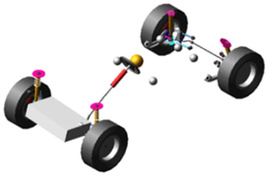
Figure 1. Multibody Dynamics Model.

The comparative analysis of the simulation results and the joint estimated values is illustrated in Figure 2, Figure 3 and Figure 4. The simulation results in Figure 2, Figure 3 and Figure 4 confirm the estimator’s performance. The estimated suspension relative velocities align closely with the reference data for all wheels, capturing the rapid changes at the ramp start without noticeable delay. For the sprung mass velocity, the algorithm successfully removes high-frequency sensor noise while preserving the actual body motion trend. Additionally, the road gradient estimation shows that the method can distinguish the road slope from the vehicle’s pitching motion, with the value converging steadily to the true 0.527.

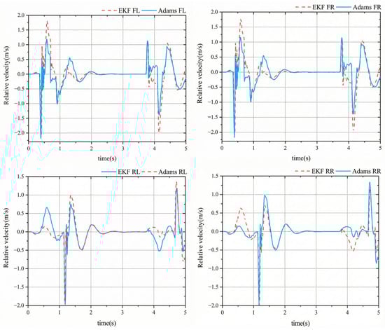
Figure 2. Simulated Values of Suspension Relative Velocity.

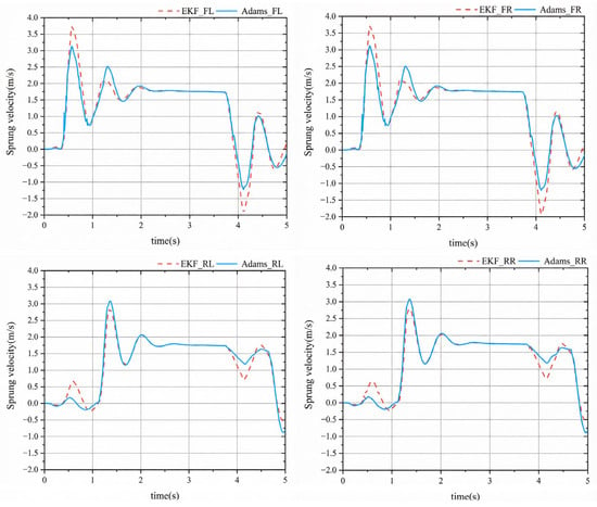
Figure 3. Simulated Values of Velocity of Sprung Mass.

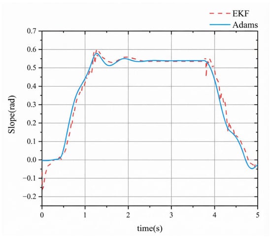
Figure 4. Simulated Values of Road gradient.

4. Experimental Procedure and Comparative Analysis

4.1. Experimental Setup

The experimental investigation was conducted using a specific model of a mid-size sedan as the subject vehicle. The experimental setup employs a strategic ‘2+1’ sensor configuration driven by system observability and sensitivity analyses, as depicted in Figure 5. Since the estimator’s accuracy is heavily dependent on the fidelity of road input measurements, two PCB Piezotronics ICP^® single-axis accelerometers are prioritized for the front unsprung masses. These sensors feature a high sensitivity of 100 mV/g and a measurement range of ±50 g, ensuring the precise capture of high-frequency road excitations without saturation. On the sprung mass, a WIT-Motion WT901 high-precision Inclinometer/IMU is installed to monitor low-frequency body attitude. It provides a static pitch/roll accuracy of 0.05° and a dynamic accuracy of 0.1°, serving as the ground truth for feedback correction. This arrangement allows the wheelbase preview model to efficiently reconstruct global vehicle states without redundant rear sensors. All data acquisition is managed by a dSPACE MicroAutoBox II real-time controller via a CAN interface, operating at a 1000 Hz sampling frequency with 16-bit resolution to ensure precise signal digitization.

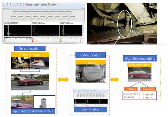
Figure 5. Experimental Procedure.

PCB accelerometers were installed at the lower mounting points of the left and right front dampers to measure the vertical acceleration of the unsprung masses. Owing to their location along the main force transmission path from the tire–road interface to the suspension system, these positions retain strong sensitivity to road-induced excitations while reducing attenuation effects introduced by compliant suspension components. The dynamic response of the sprung mass was recorded using four WIT Inertial Measurement Unit (IMU) sensors arranged symmetrically above the front and rear axles, with two sensors placed near the front axle and two in the trunk area above the rear axle. Installing the IMUs close to the axle lines allows reliable representation of the global body bounce motion and supports the separation of pitch and roll components through spatial distribution. In addition, the original vehicle configuration was equipped with four suspension height sensors located at each suspension corner, enabling measurement of the relative deflections of the four suspension assemblies for validation and reference purposes.

To facilitate the acquisition and documentation of signals pertaining to vehicle speed, pitch angle, roll angle, longitudinal acceleration, and vertical acceleration, an integrated navigation system, the CGI-220, developed by a specific company, was installed within the vehicle. The CGI-220 employs multi-sensor data fusion technology to integrate GPS with inertial measurement data, facilitating the real-time provision of high-precision information including carrier position, attitude, velocity, and other sensor outputs. The pitch and roll angles utilized in this study are measured through direct methods provided by the sensor’s internal fusion algorithms, rather than being derived via the proposed estimator.

Data from the front PCB Piezotronics accelerometers and the direct attitude outputs from the WIT-Motion IMU serve as inputs for the integrated Extended Kalman Filter (EKF) estimator. Measurements from the original vehicle height sensors and additional reference sensors function exclusively as ground truth values for validation. The optimal estimation results were obtained through a systematic parameter tuning procedure. The measurement noise covariance matrix $\mathsf{\vartheta }$ was quantitatively derived from the statistical variance of sensor signals collected under static conditions. The process noise covariance matrix $\mathsf{\omega }$ was determined through an iterative tuning process, where the elements were adjusted to minimize the Root Mean Square Error (RMSE) between the estimated states and the ground truth data provided by the height sensors. The fully tuned estimation module necessitates only three active sensors, representing a reduction in sensor requirements relative to comparable estimation methodologies found in the literature.

The experimental setup employed the dSpace/MicroAutoBox platform, which provides functionalities such as CAN communication and analog/digital signal I/O, serving as a rapid control prototyping tool. This platform allows for the direct compilation of MATLAB 2022b/Simulink models into executable programs, streamlining the development workflow. Through the ControlDesk interface, real-time parameter adjustments and data recording were performed to optimize the experiment. Beyond the experimental validation on this high-performance platform, the proposed method demonstrates significant computational efficiency. By optimizing the state vector dimension, the algorithm substantially decreases the processing demands required for matrix operations. This low computational complexity ensures that the method is not only sensor-efficient but also capable of running in real time on standard automotive Electronic Control Units (ECUs) with limited computing resources.

4.2. Analysis of Experimental Results

The experimental conditions comprised level straight driving and uphill/downhill tests conducted on a dry asphalt pavement, with a testing speed ranging from 60 to 70 km/h, as depicted in Figure 6. To evaluate the vehicle response under controlled excitation, the proving ground featured specific artificial irregularities, including sinusoidal speed bumps with an amplitude of 0.05 m and a continuous ramp section with an approximate gradient of 8%, alongside segments exhibiting mild surface unevenness to simulate real-world conditions. All tests were performed under dry weather conditions with a standardized vehicle load configuration—consisting of a driver and onboard data acquisition equipment—which was maintained throughout to ensure the repeatability of results and eliminate variability arising from mass redistribution. Finally, the precision of the state estimation algorithm was quantitatively assessed using the root mean square error (RMSE) of the relative deviation between the estimated results and the actual states.

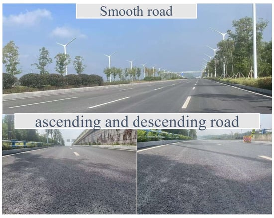
Figure 6. Experimental road section.

The estimation performance under smooth road segments is illustrated in Figure 7, Figure 8 and Figure 9. Figure 7 presents the relative vertical velocity estimation results, where the estimated trajectory (red solid line) effectively tracks the reference ground truth (blue dashed line).

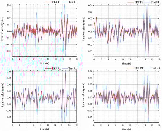
Figure 7. Relative vertical velocity estimation results.

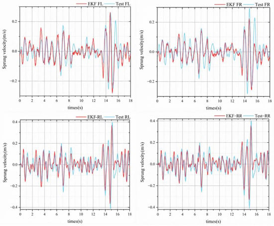
Figure 8. Sprung mass vertical velocity estimation results.

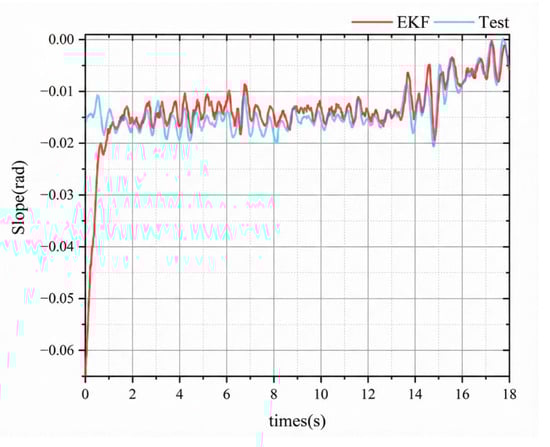
Figure 9. Values of Road gradient.

The root mean square (RMS) errors for the left front, right front, left rear, and right rear relative velocities are quantified as 0.64%, 0.42%, 0.49%, and 0.53%, respectively, as detailed in Table 3. Figure 8 depicts the sprung mass vertical velocity estimation results, yielding RMS errors of 4.41%, 4.32%, 5.94%, and 5.30% for the respective corners, which confirms the algorithm’s capability to accurately reconstruct low-frequency body heave motions while suppressing integration drift. Figure 9 illustrates the values of road gradient with a corresponding RMS error of 0.62%, highlighting the performance in successfully decoupling the road slope from the vehicle’s pitch attitude to provide precise terrain perception.

Table 3. Root Mean Square Error of Relative Error (Smooth Road Segment).

	Method	The Method in This Paper	Multi-Sensor Approach
x
${\dot{Z}}_m$		4.91	5.93
$\dot{\theta }$		0.92	1.32
$\dot{\phi }$		0.63	1.06
$\Delta {\dot{Z}}_1/\Delta {\dot{Z}}_2/\Delta {\dot{Z}}_3/\Delta {\dot{Z}}_4$		0.64/0.42/0.49/0.53	0.88/0.76/0.58/0.37
${\dot{Z}}_{s1}/{\dot{Z}}_{s2}/{\dot{Z}}_{s3}/{\dot{Z}}_{s4}$		4.41/4.32/5.94/5.30	4.63/4.38/5.83/5.31
Pavement Gradient		0.62	0.56

The reliability and adaptability of the proposed estimator under irregular road profiles are validated through Figure 10, Figure 11 and Figure 12. In the case of relative vertical velocity, the comparison shown in Figure 10 indicates that even under road irregularities, the observer (red solid line) maintains precise synchronization with the reference sensors (blue dashed line). The quantitative analysis in Table 4 records RMS errors for the four wheels at 0.42%, 0.32%, 0.25%, and 0.29%, respectively. Figure 11 presents the sprung mass vertical velocity results, where the algorithm demonstrates superior stability in capturing transient peak responses, yielding corresponding RMS errors of 2.60%, 2.52%, 3.44%, and 3.33%. This highlights the effectiveness of the EKF in handling the significant non-linearities of the suspension system. For the road gradient estimation depicted in Figure 12, the RMS error is confined to 0.43%, as detailed in Table 3, during continuous surface fluctuations.

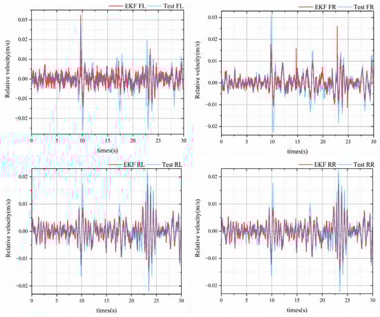
Figure 10. Relative vertical velocity estimation results.

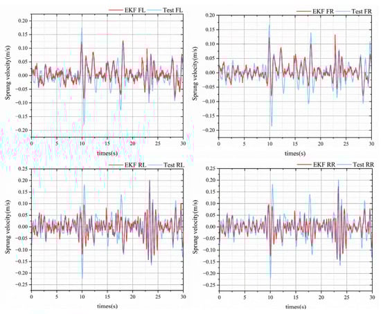
Figure 11. Sprung mass vertical velocity estimation results.

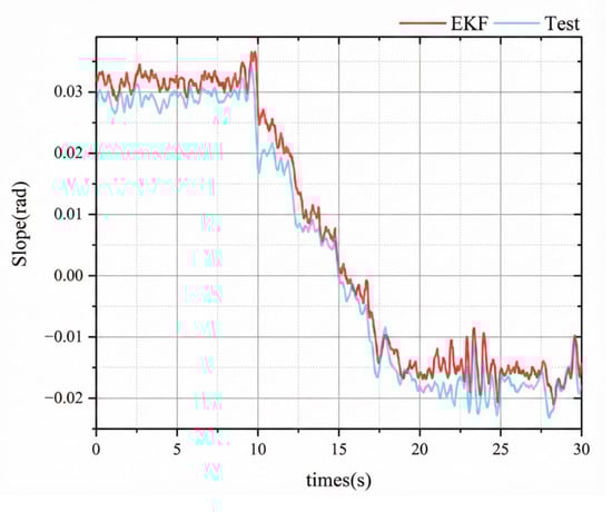
Figure 12. Values of Road gradient.

Table 4. Root Mean Square Error of Relative Error (Ascending and descending Road Segments).

	Method	The Method in This Paper	Multi-Sensor Approach
x
${\dot{Z}}_m$		3.92	4.76
$\dot{\theta }$		0.54	0.71
$\dot{\phi }$		0.66	0.84
$\Delta {\dot{Z}}_1/\Delta {\dot{Z}}_2/\Delta {\dot{Z}}_3/\Delta {\dot{Z}}_4$		0.42/0.32/0.25/0.29	0.65/0.41/0.22/0.42
${\dot{Z}}_{s1}/{\dot{Z}}_{s2}/{\dot{Z}}_{s3}/{\dot{Z}}_{s4}$		2.60/2.52/3.44/3.33	3.1/3.12/3.02/3.56
Pavement Gradient		0.43	0.56

The experimental findings derived from the vehicle’s assessment over two distinct roadway segments reveal that the root mean square (RMS) errors for the estimated relative velocities of the suspension remain consistently below 0.7%. Likewise, the RMS errors for the absolute velocities of the springs are all below 6%, while the RMS errors for gradient estimation do not exceed 0.7%. The overall estimation accuracy of the proposed algorithm is superior to that of multi-sensor schemes. Multi-sensor approaches typically require more than five sensors, which leads to higher costs, and the superposition of noise from data sources can cause estimation errors. In contrast, the proposed algorithm utilizes a configuration of only two accelerometers and a single IMU. This setup reduces costs and avoids noise accumulation, resulting in better overall estimation accuracy. These results substantiate the efficacy of the extended Kalman filter-based joint state estimation algorithm, which incorporates wheelbase previewing, in accurately estimating suspension-related states and road gradients in real-world vehicular applications.

5. Discussion

The wheelbase preview assumption, which posits that rear wheel inputs replicate front wheel inputs with a time delay, is highly dependent on the vehicle’s operating conditions. Empirical evidence indicates that this assumption achieves high estimation accuracy during longitudinal maneuvers on well-paved roads, such as straight-line acceleration and ramp climbing, where the root mean square (RMS) error of relative velocity between the front and rear wheels remains below 0.7%. However, its reliability decreases under dynamic maneuvers involving significant lateral acceleration. During sharp cornering or aggressive lane changes, the rear axle trajectory deviates from the front axle path, weakening the spatial correlation required for accurate preview-based estimation. Furthermore, neglecting wheel unsprung mass dynamics and adopting a rigid point contact model limits the estimator’s performance on high-frequency or uneven surfaces. While these simplifications reduce computational load and facilitate real-time implementation, they are inherently better suited to low-slip, low-frequency road excitations. Under extreme handling or complex terrain conditions, the limitations of this assumption cannot be ignored, and incorporating more comprehensive vehicle dynamics modeling becomes necessary to ensure accurate and reliable state estimation.

6. Conclusions

This study introduces a joint estimation algorithm based on the Kalman Filter (KF) designed to concurrently estimate critical parameters essential for optimizing vehicle dynamic performance and enhancing safety control. These parameters include the suspension spring velocity, the relative velocity between the sprung and unsprung masses, and the road gradient. The proposed methodology significantly reduces the number of estimators required, thereby minimizing computational overhead during integration and improving overall system efficiency. The algorithm utilizes input signals comprising vehicle speed, longitudinal and vertical accelerations, vertical velocities of both front and rear axles, as well as pitch and roll angles of the vehicle. The feasibility of the algorithm is rigorously validated through a synergistic simulation approach that integrates Simulink and Adams software. In the empirical testing phase, this research harnesses the CAN communication capabilities of the dSpace/MicroAutoBox platform, ensuring seamless integration with MATLAB/Simulink for the application of the joint estimation algorithm in a real-world vehicle setting. The proposed methodology employs a “2 + 1” sensor configuration strategy, which markedly reduces the number of required sensors compared to conventional suspension state estimation techniques. This approach not only simplifies the sensor deployment process but also decreases both experimental costs and the expenses associated with subsequent commercialization, thereby offering a distinct low-cost advantage while effectively mitigating the noise accumulation often present in integration-based methods. Results from the experiments indicate that the EKF-based joint estimation algorithm is capable of accurately estimating critical dynamic parameters of both front and rear suspensions, as well as the road gradient, thus validating its efficacy and practicality in real-world applications. Furthermore, the method demonstrates significant adaptability to different vehicle types, such as trucks and electric vehicles, requiring only the adjustment of parameters like wheelbase and mass for migration. However, a limitation exists regarding the linear assumptions; specifically, under high-frequency excitations or extreme working conditions, higher sampling rates or nonlinear tire models become requisite to maintain estimation fidelity. Future research will focus on extending model fidelity by incorporating vertical wheel dynamics and nonlinear tire characteristics, thereby broadening the estimator’s applicability in complex terrains and high-dynamic handling limits. The outcomes of this study hold significant implications for advancing the intelligent control of vehicle suspension systems, thereby enhancing driving comfort, stability, and safety.

References

- Papaioannou, G.; Koulocheris, D.; Velenis, E. Skyhook control strategy for vehicle suspensions based on the distribution of the operational conditions. Proc. Inst. Mech. Eng. Part D J. Automob. Eng. 2021, 235, 2776–2790. [Google Scholar] [CrossRef]
- Hu, Y.; Chen, M.Z.Q.; Sun, Y. Comfort-oriented vehicle suspension design with skyhook inerter configuration. J. Sound Vib. 2017, 405, 34–47. [Google Scholar] [CrossRef]
- Bi, B.W.; Xiao, F. The Implementation of Skyhook Control for Semi-Active Suspension Based on Vi-CarRealTime. Appl. Mech. Mater. 2015, 713, 748–751. [Google Scholar] [CrossRef]
- Liu, Y.; Cui, D. Vehicle state estimation based on adaptive fading unscented kalman filter. Math. Probl. Eng. 2022, 2022, 7355110. [Google Scholar] [CrossRef]
- Zoljic-Beglerovic, S.; Luber, B.; Stettinger, G.; Müller, G.; Horn, M. Parameter identification for railway suspension systems using Cubature Kalman filter. In Advances in Dynamics of Vehicles on Roads and Tracks, Proceedings of the 26th Symposium of the International Association of Vehicle System Dynamics, IAVSD 2019, Gothenburg, Sweden, 12–16 August 2019; Springer International Publishing: Cham, Switzerland, 2020; pp. 128–132. [Google Scholar]
- Li, J.; Wang, L.; Miao, Y.; Tong, X.; Ye, Z. Road Roughness Detection Based on Discrete Kalman Filter Model with Driving Vibration Data Input. Int. J. Pavement Res. Technol. 2023, 18, 480–492. [Google Scholar] [CrossRef]
- Hao, S.; Luo, P.; Xi, J. Estimation of vehicle mass and road slope based on steady-state Kalman filter. In Proceedings of the 2017 IEEE International Conference on Unmanned Systems (ICUS), Beijing, China, 27–29 October; pp. 582–587.
- Kim, M.S.; Kim, C.I.; Lee, K.S. Vehicle dynamics and road slope estimation based on cascade extended kalman filter. J. Inst. Electron. Inf. Eng. 2014, 51, 208–214. [Google Scholar] [CrossRef]
- Jeyed, H.A.; Ghaffari, A. Nonlinear estimator design based on extended Kalman filter approach for state estimation of articulated heavy vehicle. Proc. Inst. Mech. Eng. Part K J. Multi-Body Dyn. 2019, 233, 254–265. [Google Scholar]
- Yuhao, H. Estimation of Vehicle Status and Parameters Based on Nonlinear Kalman Filtering. In Proceedings of the 2022 6th International Conference on Robotics and Automation Sciences (ICRAS), Wuhan, China, 9–11 June 2022; pp. 200–205. [Google Scholar]
- Wang, Y. Extended kalman filter based state estimation of formula student autonomous racing. In Proceedings of the Ninth International Conference on Mechanical Engineering, Materials, and Automation Technology (MMEAT 2023), Dalian, China, 9–11 June 2023; Volume 12801, pp. 1549–1555. [Google Scholar]
- Alshawi, A.; De Pinto, S.; Stano, P.; van Aalst, S.; Praet, K.; Boulay, E.; Ivone, D.; Gruber, P.; Sorniotti, A. An Adaptive Unscented Kalman Filter for the Estimation of the Vehicle Velocity Components, Slip Angles, and Slip Ratios in Extreme Driving Manoeuvres. Sensors 2024, 24, 436. [Google Scholar] [CrossRef] [PubMed]
- Jin, X.J.; Yin, G.; Hanif, A. Cubature kalman filter-based state estimation for distributed drive electric vehicles. In Proceedings of the 2016 35th Chinese Control Conference (CCC), Chengdu, China, 27–29 July 2016; pp. 9038–9042. [Google Scholar]
- Singh, K.B.; Taheri, S. Integrated state and parameter estimation for vehicle dynamics control. Int. J. Veh. Perform. 2019, 5, 329–376. [Google Scholar] [CrossRef]
- Rodríguez, A.J.; Sanjurjo, E.; Pastorino, R.; Naya, M.Á. State, parameter and input observers based on multibody models and Kalman filters for vehicle dynamics. Mech. Syst. Signal Process. 2021, 155, 107544. [Google Scholar] [CrossRef]
- Huang, C.; Du, X.; Xue, J.; Fu, J.; Wen, M.; Yu, M. Kalman Filtering for Sprung Mass Velocity Estimation of Magnetorheological Suspension for All -Terrain Vehicle. In Proceedings of the 2019 Chinese Control and Decision Conference (CCDC), Nanchang, China, 3–5 June 2019; pp. 1097–1101. [Google Scholar]
- Wang, Z.; Dong, M.; Qin, Y.; Du, Y.; Zhao, F.; Gu, L. Suspension system state estimation using adaptive Kalman filtering based on road classification. Veh. Syst. Dyn. 2017, 55, 371–398. [Google Scholar] [CrossRef]
- Kim, G.W.; Kang, S.W.; Kim, J.S.; Oh, J.S. Simultaneous estimation of state and unknown road roughness input for vehicle suspension control system based on discrete Kalman filter. Proc. Inst. Mech. Eng. Part D J. Automob. Eng. 2019, 234, 1610–1622. [Google Scholar] [CrossRef]
- Jeong, K.; Choi, S.B. Vehicle suspension relative velocity estimation using a single 6-D IMU sensor. IEEE Trans. Veh. Technol. 2019, 68, 7309–7318. [Google Scholar] [CrossRef]
- Lin, C.; Liu, W.; Ren, H. State estimation based on unscented Kalman filter for semi-active suspension systems. J. Vibroeng. 2016, 18, 446–457. [Google Scholar]
- Zhao, J.; Hua, X.; Cao, Y.; Fan, L.; Mei, X.; Xie, Z. Design of an integrated controller for active suspension systems based on wheelbase preview and wavelet noise filter. J. Intell. Fuzzy Syst. 2019, 36, 3911–3921. [Google Scholar] [CrossRef]
- Xie, Z.; Wong, P.K.; Zhao, J.; Xu, T.; Wong, K.I.; Wong, H.C. A Noise-Insensitive Semi-Active Air Suspension for Heavy-Duty Vehicles with an Integrated Fuzzy-Wheelbase Preview Control. Math. Probl. Eng. 2013, 2013, 121953. [Google Scholar] [CrossRef]
- Li, P.; Lam, J.; Cheung, K.C. Multi-objective control for active vehicle suspension with wheelbase preview. J. Sound Vib. 2014, 333, 5269–5282. [Google Scholar] [CrossRef]
- Kwon, B.; Kang, D.; Yi, K. Wheelbase preview control of an active suspension with a disturbance-decoupled observer to improve vehicle ride comfort. Proc. Inst. Mech. Eng. Part D J. Automob. Eng. 2020, 234, 1725–1745. [Google Scholar] [CrossRef]
Disclaimer/Publisher’s Note: The statements, opinions and data contained in all publications are solely those of the individual author(s) and contributor(s) and not of MDPI and/or the editor(s). MDPI and/or the editor(s) disclaim responsibility for any injury to people or property resulting from any ideas, methods, instructions or products referred to in the content. |
© 2026 by the authors. Licensee MDPI, Basel, Switzerland. This article is an open access article distributed under the terms and conditions of the Creative Commons Attribution (CC BY) license.