Abstract
To achieve the automation and intelligence of mining equipment, it is essential to address the challenge of autonomous driving, with the core task being how to navigate safely from the starting point to the mining area endpoint. This paper proposes a boundary-aware multi-point preview control algorithm to tackle the strong dependency on predefined paths and the lack of foresight in the autonomous driving of underground articulated mining vehicles in highly confined underground spaces. The algorithm determines the driving direction by calculating the vehicle’s real-time state and LiDAR data, previewing road conditions without relying on preset path planning. Experiments conducted in a ROS Noetic/GAZEBO 11 simulation environment compared the proposed method with single-point and two-point preview algorithms, validating the effectiveness of the boundary-aware multi-point preview control. The results show that the proposed control strategy yields the lowest lateral deviation and the highest steering smoothness compared to single-point and two-point preview algorithms; it also outperforms the standard multi-point preview algorithm. This demonstrates its superior performance. Specifically, the proposed boundary-aware multi-point preview algorithm outperformed other methods in terms of steering smoothness and stability, significantly enhancing the vehicle system’s adaptability, robustness, and safety.
1. Introduction
With the continuous development of modern mining technology, underground mining vehicles are playing an increasingly important role in mining transportation, loading, and hauling operations [1]. Underground mining faces numerous safety hazards, such as high humidity, high temperatures, collapses, and water inflow. These harsh conditions not only severely constrain the efficiency of resource extraction but also pose significant safety risks to underground workers [2]. The automation level of currently used mining equipment remains low, resulting in insufficient productivity and hindering the further development of the underground mining industry. To address these challenges, developing unmanned mining equipment for deep resources has become an urgent need [3].
Among mining equipment, articulated vehicles stand out for their maneuverability, flexibility, and efficiency, making them essential for highly confined underground spaces. Intelligent underground articulated vehicles enable unmanned operation and autonomous driving in mine tunnels while accurately controlling the bucket position, movement trajectory, and load. Moreover, they monitor changes in the surrounding environment in real time, issue timely warnings, and implement measures to mitigate safety hazards such as collisions and landslides, ensuring safe and efficient operation [4].
Significant advancements have been achieved in the research on intelligent underground mining vehicles worldwide. Autonomous driving control can effectively prevent vehicle disruptions caused by obstacles, terrain changes, complex road conditions, and other factors, ensuring safe operation. It relies on highly integrated perception and decision-making capabilities. In this process, path tracking control methods play a critical role. Through path tracking algorithms, vehicles can effectively execute predetermined trajectories in complex, confined underground spaces, adjusting their motion state in real time to cope with environmental changes and external disturbances, thereby ensuring the safety and stability of autonomous driving.
Model-based path-tracking methods rely on the vehicle’s kinematic or dynamic characteristics, enabling prediction and compensation for potential deviations between the actual motion and the planned path. FUE et al. [5] improved the pure pursuit algorithm by considering the steering delay of articulated vehicles and introducing error correction parameters. DEKKER et al. [6] introduced an iterative learning algorithm based on feedback linearization control. By adjusting the control algorithm parameters based on the error and control inputs from the previous tracking of the same path, the approach enabled self-correction of errors during tracking. This improvement enhanced the tracking accuracy and robustness of unmanned underground loaders during repetitive operations. NAYL et al. [7] designed a novel sliding mode control based on the nonlinear error kinematic model of articulated steering vehicles. This approach features a new nonlinear continuous sliding surface that, compared to traditional sliding surfaces, is distributed across all phase planes, effectively reducing chattering during the tracking control process. YANG et al. [8] incorporated external disturbances and model uncertainties into the standard sliding mode control algorithm, using this to compensate for the disturbance effects on the curvature of the reference trajectory. TIAN et al. [9] designed an LQR-based differential coordination control method using a two-degree-of-freedom dynamic model of articulated steering vehicles. The design considered the centroid sideslip angle deviation and yaw rate deviation of the front vehicle body, improving both accuracy and stability. YU et al. [10] utilized intelligent clustering algorithms such as Genetic Algorithm, Ant Colony Algorithm, and Particle Swarm Optimization to optimize the Q and R matrix parameters, improving the optimal performance of LQR control. ZHOU et al. [11] improved the traditional MPC algorithm by using Genetic Algorithm to obtain optimal prediction and control time-domain parameters in real time within the system’s sampling frequency, enhancing the smoothness and stability of path tracking. SHI et al. [12] developed an Adaptive Model Predictive Control approach based on the kinematic and dynamic tracking error model of autonomous wheeled loaders, incorporating the effects of path curvature disturbances. This improved tracking performance on paths with varying curvatures. BAI et al. [13] proposed a Nonlinear Model Predictive Control (NMPC) approach using a nonlinear kinematic model of articulated vehicles as the predictive model. This addressed the performance degradation of traditional linearized MPC when the vehicle’s longitudinal speed is too high.
In the field of model-free control, GUAN et al. [14] designed a PID control algorithm with hyperparameters that can be dynamically tuned using intelligent optimization algorithms. This enabled the articulated vehicle to accurately track the path under real uneven road conditions. The fuzzy PID control designed by TAN et al. [15] reduced the oscillation effects of articulated vehicles in underground tunnel environments. DOU et al. [16] developed a relative navigation control law based on neural networks, enhancing navigation control accuracy by establishing a steering kinematic model. WIBERG et al. [17] explored the application of reinforcement learning in heavy articulated vehicles within a virtual environment and validated its feasibility in rugged terrain. ZHAO et al. [18] combined traditional navigation with Deep Q-Networks, optimizing the articulation angle adjustment, and verified the training effect of their algorithm in a virtual tunnel.
Existing path tracking methods aim to enhance accuracy, robustness, and adaptability to complex environments. Model-based approaches leverage precise dynamics and control but struggle with environmental changes, while model-free methods excel in adaptability through error correction and self-learning. However, these methods primarily focus on minimizing deviations between the actual trajectory and the desired path. They rely on prior planning and a predefined expected path, aiming to improve control performance by reducing tracking errors and aligning the vehicle’s motion more closely with the planned trajectory. They have a strong dependence on the expected path and lack foresight.
To address these challenges in highly constrained underground environments, this paper proposes a boundary-aware multi-point preview control algorithm that directly leverages real-time LiDAR data to dynamically determine the vehicle’s driving direction and speed. By predicting upcoming road conditions and eliminating dependence on predefined paths, the algorithm enhances the system’s adaptability to environmental changes.
To sum up, the main contributions of this article are threefold:
- By utilizing a preview control model inspired by human driving habits, this paper proposes a boundary-aware multi-point preview control algorithm for autonomous articulated vehicles in highly constrained underground environments. The algorithm directly leverages real-time LiDAR data to dynamically determine the vehicle’s driving direction and speed.
- The algorithm enhances the steering smoothness by dynamically adjusting the gain of the control deviations. The system can sense the status changes of the articulated vehicle in real time and automatically adjust the gain parameters to adapt to different working conditions in underground tunnels, ensuring smoothness and accuracy in the steering process.
- A speed decision-making scheme based on multi-point preview deviation is proposed, which dynamically adjusts the articulated vehicle’s speed according to environmental changes in confined underground tunnels.
2. Problem Definition
This section establishes the kinematic model of the underground articulated vehicle and analyzes its control requirements for underground, highly constrained spaces. Relevant control metrics are then defined to evaluate its autonomous driving behavior in such tunnels.
2.1. Kinematic Model
The articulated vehicle employs a unique steering mechanism where the front and rear sections of the vehicle rotate relative to each other through two hydraulic cylinders connected at the articulation point. This generates a relative yaw angle, allowing the vehicle to steer easily in complex or narrow environments.
In Figure 1, and represent the centers of the front and rear vehicle bodies, respectively. (,) and (,) are the coordinates of and . and represent the velocities of and . is the articulation point. is the articulation angle. and are the heading angles of the front and rear vehicle bodies, respectively. and represent the distances from point to point and from point to point , respectively. is the wheelbase. The dashed lines indicate the turning radius.
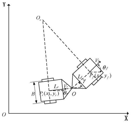
Figure 1.
Kinematic model of an articulated vehicle.
Ignoring the motion in the vertical direction, the motion of the articulated vehicle can be simplified as the plane motion of two articulated rigid bodies, with the following relationship at the articulation point:
Therefore, the following can be derived from Equation (1):
By simplifying Equation (2), the following result is obtained:
Equation (4) can be obtained from Figure 1:
Taking the derivative of both sides of Equation (4) gives the following:
Substituting the above equation into Equation (5) yields the following:
Since the tire side slip has been ignored, it can be concluded as follows:
The kinematic model of the articulated vehicle equipment can be obtained as follows:
2.2. Control Requirements for Autonomous Driving in Underground and Highly Constrained Spaces
Real-time perception and environmental adaptability: The complexity of underground and highly constrained spaces requires articulated vehicles to perceive road information ahead in real time, including uneven terrain, sudden obstacles, and special ground conditions such as slippery or gravel-covered surfaces. The vehicle needs to use a combination of sensors, such as LiDAR and vision sensors, to gather environmental data in real time, quickly adapt to changes in the environment, and ensure the stability of autonomous driving.
Dynamic control and stability assurance: The uneven terrain and frequent directional adjustments in underground and highly constrained spaces require the vehicle to have a highly robust dynamic control system. The vehicle needs to continuously monitor its driving status and dynamically adjust control parameters such as speed and steering angle to ensure good driving stability in complex terrain, preventing derailments or overturning accidents caused by delays or inaccurate control.
Look-ahead and predictive control capability: Due to the unpredictability of terrain and obstacles in underground and highly constrained spaces, the vehicle’s control system should possess look-ahead capabilities. Anticipating upcoming road conditions and potential obstacles can help adjust driving direction and speed in advance. This “look-ahead” control can effectively mitigate the impact of delays or uncertainties in road conditions.
2.3. Control Metrics for Autonomous Driving
In the operation of articulated vehicles in underground and highly constrained spaces, this paper no longer focuses on traditional path planning and tracking issues. Instead, it takes the distance between the articulated vehicle and the walls of the constrained space as a key indicator for evaluating driving quality. At the same time, the articulation angle of the front vehicle body and its angular velocity are used as indicators to evaluate driving smoothness, ensuring the safe and stable operation of the articulated vehicle in underground and highly constrained spaces.
In Figure 2, represents the distance from the articulation point to the left wall, represents the distance from the articulation point to the right wall, denotes the articulation point, and indicates the position where the LiDAR is installed.
where and are the coordinates of the right and left walls, respectively, as obtained by the LiDAR on the articulated vehicle. , are the coordinates of the articulation point of the vehicle. The bidirectional proximity is used as an indicator to evaluate the safety of the vehicle’s driving. A smaller value of reflects better safety, as it indicates the vehicle is maintaining an appropriate and balanced distance from both walls, reducing the risk of collision and ensuring stable and secure operation. The articulation angle velocity is used as the indicator to evaluate whether the vehicle’s driving is smooth and stable.
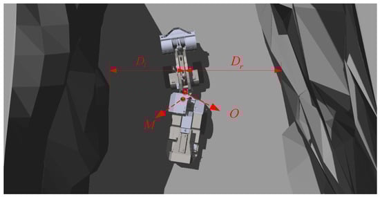
Figure 2.
Articulated vehicle’s position and key metrics.
In traditional path tracking methods, a reference path is usually given, and the vehicle is controlled to follow this path in order to achieve precise driving along a predefined trajectory for the articulated vehicle. This method mainly relies on path planning algorithms by generating an optimal reference path, and real-time adjustment of the vehicle’s steering angle and speed is made based on the error between the vehicle’s current position and the reference path, ensuring the vehicle continuously follows the reference path.
In underground and highly constrained spaces, traditional path tracking methods face severe challenges. The complex tunnel environment—featuring narrow curves, local obstacles, and uneven surfaces—makes path planning and tracking difficult. Even with a predefined path, the articulated vehicle’s motion is influenced by inertia, steering response, and tunnel wall constraints, often causing yawing. Moreover, the articulated structure between the front and rear bodies results in large relative yaw angles during steering, imposing stricter stability requirements than conventional vehicles.
To address these issues, this paper proposes a multi-point preview deviation-based autonomous driving algorithm. Unlike single look-ahead approaches, it dynamically selects multiple preview points to obtain richer environmental feedback. This enhances predictive capability and compensates for the slow response of traditional algorithms in handling sudden changes, thereby improving safety and stability in confined underground spaces.
3. Boundary-Aware Multi-Point Preview Control Algorithm
This paper constructs a multi-point preview model, unlike traditional preview models that rely on a single or a limited number of target points for decision-making [19]. The traditional path tracking algorithms tend to result in delayed responses to sudden situations in underground and highly constrained spaces. The multi-point preview model [20] uses multiple look-ahead points distributed at different positions and combines this information using algorithms like weighted averaging or optimal prediction to forecast future environmental changes, addressing delays and achieving optimal control for the vehicle. This ensures that the vehicle can respond in real time to changes in the highly constrained space and challenges in the complex underground environment. It effectively addresses yaw instability and the lack of foresight in autonomous driving. Figure 3 illustrates the overall algorithm framework.
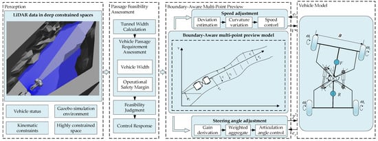
Figure 3.
Algorithm framework.
In the proposed framework, LiDAR perception is used to extract geometric constraints of the drivable corridor rather than performing explicit semantic classification. Specifically, both tunnel boundaries and obstacles are uniformly treated as geometric constraints in the form of spatial boundary information.
In practical underground mining operations, tunnel dimensions may vary significantly due to geological deformation or localized collapses, resulting in intermittently narrow passages that are not safely traversable. The proposed framework explicitly addresses this challenge through a traversability feasibility assessment, which continuously evaluates the available clearance between the vehicle and the surrounding tunnel boundaries.
Specifically, the effective drivable corridor width, derived from LiDAR-based boundary detection, is monitored in real time and compared with the minimum width required for safe vehicle passage. This minimum width accounts for the articulated vehicle’s body envelope and incorporates a predefined safety margin to compensate for control uncertainties and environmental disturbances. When the available corridor width falls below this threshold, the corresponding region is classified as non-traversable. In such cases, the control algorithm suppresses speed commands and initiates a conservative speed reduction or stopping strategy, thereby preventing the vehicle from entering unsafe or impassable areas.
When an underground mining articulated vehicle navigates through subterranean tunnels, the LiDAR system mounted on the front body scans the surrounding tunnel environment, collecting a series of LiDAR data points representing the tunnel walls. This data is then input into the multi-point preview model for processing, where a set of deviations is calculated.
These deviations are used to adjust the preview-based steering angle and speed decisions. The computed steering angle and speed are subsequently transmitted to the vehicle model.
3.1. Steering Control
To address the directional control problem for vehicles in underground and highly constrained spaces, or in complex curved road sections, this paper designs a steering control module by continuously adjusting the articulation angle in real time. This ensures stable steering and posture when making sharp turns, driving through narrow tunnels, or navigating uneven surfaces.
To enable the multi-point preview model to maintain better lane-keeping capability, a special point called the guide point is defined. The subsequent tunnel wall points are used as prediction points. The heading angle deviation of the guide point (the difference between the angle formed by the guide point and the center of the front vehicle body and the vehicle’s heading angle) is used as the state feedback variable. In comparison, the lateral deviation of the subsequent points from the lines formed by the vehicle’s heading direction is used as prediction data.
As shown in Figure 4, during the look-ahead process in highly confined underground spaces, the deviation input includes deviation information from a series of points, ranging from near to far. The heading angle deviation of the guide point can, if necessary, be integrated or differentiated as additional input to improve the accuracy of the vehicle’s path tracking. Additionally, some state feedback values are also used as inputs to the controller.

Figure 4.
Boundary-aware multi-point preview model.
When the articulated vehicle moves through a rough and highly confined space with a long look-ahead distance, the multi-point preview model calculates a series of deviation values (, ,……, ). The current vehicle heading angle is , which determines the direction of the look-ahead line, thereby affecting the calculation of the LiDAR data points. Define the variable as the tunnel wall data feedback received from the -th LiDAR ray, and as the angle of the i-th LiDAR ray in the vehicle’s coordinate system. denotes the preview angle deviation between the vehicle and the guide point.
Then, the deviations (, ,……, ) at each tunnel wall can be expressed as follows:
The guide point can be expressed as follows:
In Equation (11), represents a specific LiDAR angle, while represents the angle symmetrically opposite to it. and are the feedback data from the LiDAR rays corresponding to angles and , respectively.
Define as the preview angle deviation of the guide point, which is expressed as follows:
By setting and dynamically adjusting the gain , and combining a series of lateral errors (, ,……, ), the desired articulation angle can be calculated, which is expressed as follows:
where is the gain control function, which is expressed as follows:
From Equation (14), it can be observed that as gets closer to the vehicle’s heading direction (the 90th ray), becomes larger. This indicates that the information from points closer to the center in front of the vehicle is more significant and will have a greater influence on the steering angle decision, which will be further validated in the subsequent process variable analysis.
As seen from Equation (13), the nonlinearity of the control algorithm lies in the second term. The gain value of the second term is extracted and defined as :
It can be seen that variations in the preview feedback data will result in different gain control functions , causing the gain value calculated each time to vary, thus making the computed steering angle more flexible. Since is a function of , the gain value calculated for points farther away may be larger, indicating that the steering control is more sensitive to information from distant points.
3.2. Speed Control
In addition to steering control, speed control is equally critical for navigating highly confined spaces. By integrating the guidance point information generated by the multi-point preview model with dynamic obstacle detection data, the vehicle’s speed is adjusted in real time. Based on vehicle kinematic control theory, the speed decision module dynamically calculates appropriate speeds using parameters such as vehicle state, road complexity, and the distance to upcoming obstacles. To enhance the model’s robustness, the speed control employs an adaptive regulation method, allowing it to anticipate road condition changes in advance. This approach enables acceleration on flat sections and deceleration in hazardous or narrow passages.
Let represents the desired speed value. The speed control process leverages the input from multi-point preview deviations to sense changes in the road environment, particularly changes in curvature, to determine an appropriate speed. Here, speed decision-making is controlled using the cumulative value of lateral deviations from the multi-point preview. can be calculated using the following equation:
In Equation (16), represents the speed control gain, and is a proportional constant used to limit the range of speed variations. The numerator is the sum of LiDAR distances, a relatively constant value. In the denominator, is the only variable. When road curvature changes, the most noticeable effect is the variation in . If this variation occurs at a distant point, the larger preview distance at that point leads to a greater product of and . Consequently, the sum of the denominator increases significantly, resulting in a rapid decrease in the overall value of the equation, exhibiting behavior akin to an inverse proportional function.
Through analysis, it is evident that the speed equation does not directly reflect the absolute information of road curvature; rather, it captures the trend of curvature changes. Specifically, when road curvature changes at distant points, responds with a quick reduction, enabling the vehicle to decelerate before entering the curve.
Although the preview model is formulated in the spatial domain, vehicle speed implicitly determines the temporal meaning of preview information. By dynamically reducing speed in response to increasing multi-point preview deviations, the proposed method effectively enlarges the available preview time horizon, thereby ensuring sufficient time for smooth articulation angle adjustment and suppressing yaw oscillations.
3.3. Passage Feasibility Assessment
In highly confined underground mining environments, the geometric width of the drivable corridor may vary significantly due to geological deformation, tunnel irregularities, or localized collapses. To prevent the articulated vehicle from entering unsafe or impassable regions, a passage feasibility assessment mechanism is incorporated into the proposed framework.
Based on the boundary-aware multi-point preview model, symmetric LiDAR rays are used to evaluate the lateral clearance of the corridor at multiple preview cross-sections ahead of the vehicle. Specifically, for each preview ray pair , the lateral deviations between the vehicle centerline and the left and right tunnel boundaries are denoted as and , respectively. By combining each pair of symmetric deviations, an effective corridor width estimate at the corresponding preview cross-section can be obtained.
To conservatively evaluate the traversability of the upcoming passage, the minimum effective corridor width among all preview sections is selected as the passage feasibility indicator , which is defined as follows:
It should be noted that does not necessarily represent the true physical tunnel width, but rather a conservative geometric approximation derived from LiDAR perception that is sufficient for real-time safety assessment.
To account for uncertainties arising from control errors, actuator delays, LiDAR measurement noise, and vehicle attitude disturbances caused by uneven terrain, a predefined safety margin is introduced into the width evaluation process. The minimum safe corridor width required for vehicle passage is defined as follows:
where denotes the effective body envelope width of the articulated vehicle, considering its geometric dimensions and articulation characteristics; is a predefined safety margin used to compensate for the aforementioned uncertainties, in this study = 0.6.
The passage feasibility is determined by comparing the LiDAR-derived corridor width indicator with the minimum required safe width . If , the passage is classified as traversable, and the vehicle is allowed to proceed under the nominal speed control strategy. If , the passage is classified as non-traversable, indicating insufficient clearance for safe vehicle operation.
In the non-traversable case, the control algorithm suppresses the nominal speed command and triggers a conservative speed response, such as gradual deceleration or a complete stop. This mechanism effectively prevents the articulated vehicle from entering unsafe or impassable regions and enhances operational safety in highly constrained underground environments.
4. Simulation Environment Construction
This study developed a simulation platform for underground articulated mining vehicles using ROS Noetic/GAZEBO 11 to test and evaluate the performance of their autonomous driving systems in highly confined underground spaces. Integrating advanced simulation technologies with practical application requirements, the platform employs high-precision physical modeling and environmental sensing to realistically simulate articulated vehicles navigating complex and constrained underground spaces. This simulation platform enables comprehensive validation of the autonomous driving system’s ability to navigate and adjust speed in narrow and dynamically changing underground environments.
4.1. Articulated Vehicle
An articulated vehicle model is defined using URDF (Unified Robot Description Format). The URDF describes the articulated vehicle model within the GAZEBO simulation platform, including links, joints, kinematic/dynamic parameters, visualization, and collision detection models [21]. A 3D model was created in SolidWorks 2022, with reference points and coordinate systems added to define the positions and orientations of links and joints. The URDF export configuration in SolidWorks included naming conventions, selection of components, specification of reference axes, joint types, and link properties. Upon completing the configuration, the URDF model file was exported for simulation and control in ROS Noetic, as shown in Figure 5.
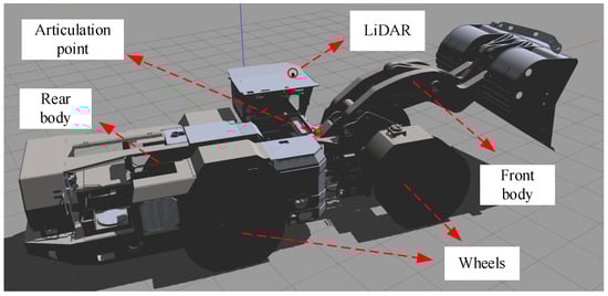
Figure 5.
Articulated vehicle simulation model.
In this study, the articulated vehicle model is developed based on a four-ton underground mining articulated vehicle. The key structural and physical parameters used in the simulations are summarized in Table 1, which provides a clear and concise description of the vehicle configuration. The following control parameters are adopted in the model: , = 0.2, = 5000, = 50.

Table 1.
Parameters of the articulated mining vehicle model.
4.2. Transport Route
A simulated environment for the operation of articulated vehicles within underground and highly constrained spaces was established on the GAZEBO platform, as shown in Figure 6. The original underground tunnel maps were filtered and simplified according to simulation requirements, retaining key features such as main tunnels, geometric shapes, dimensions, orientations, intersections, and gradient changes. Using the information on tunnel wall lengths and dimensions, preliminary environment modeling was performed in SolidWorks to ensure geometric consistency and dimensional accuracy. The models created in SolidWorks were then exported and imported into Blender, where irregular and non-uniform tunnel wall geometries commonly encountered in underground mining environments were further refined. The finalized models were imported into the GAZEBO platform for simulation purposes. This approach, utilizing Blender’s flexibility for complex surface modeling, was adopted to enhance modeling efficiency while ensuring geometric fidelity.
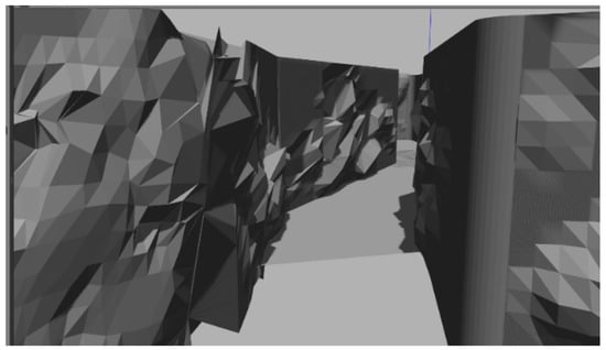
Figure 6.
Highly constrained space simulation in the GAZEBO platform.
To validate the effectiveness and robustness of the control algorithm proposed in this paper, simulation tests were conducted using the high-precision environmental simulation capabilities of GAZEBO. Specifically, the test environment was configured to resemble a real underground metallic mine tunnel, with the transport route selected from a section of the -645 level in the Xishan mining area of Sanshandao Gold Mine, Shandong Gold Mining (Laizhou) Co., Ltd. The environment included two distinct road conditions, as shown in Figure 7, with two key locations: point A (loading point) and point F (unloading point). Point A simulated the initial position where the articulated vehicle loads ore, while point F represented the target destination for unloading the ore. The figure includes yellow arrows indicating the vehicle’s driving direction and red dots representing key turning points along the route, providing visual guidance of the vehicle’s planned trajectory. The test environment was configured to resemble a real underground metallic mine tunnel, featuring complex and irregular terrain characteristics such as curves, narrow passages, and potential obstacles. This environment posed significant challenges to the vehicle’s autonomous driving capabilities, particularly in steering, acceleration, braking, and speed control.
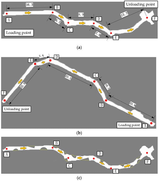
Figure 7.
Map of the underground tunnel. (a) Transport Route 1; (b) Transport Route 2; (c) Transport Route 3.
Figure 7c illustrates a more challenging road condition constructed based on the baseline environment shown in Figure 7a, where additional obstacles were deliberately introduced along the tunnel. These obstacles include localized protrusions and partial narrowing of the tunnel cross-section, which collectively increase the geometric complexity and roughness of the driving corridor. Figure 8 shows the detailed view of Transport Route 3. The blue area in front of the vehicle represents the radar’s detection zone, where deep blue lines indicate rays that receive radar feedback, and light blue lines indicate rays beyond the radar’s detection range without feedback.
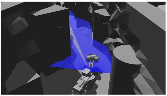
Figure 8.
Detailed View under Transport Route 3.
4.3. Sensor
In the simulation experiments, the primary sensor used is the LiDAR, which captures 2D planar data while ignoring 3D depth information. The configuration parameters of the LiDAR in Gazebo are detailed in Table 2:
Table 2.
Sensor configuration.
4.4. Control Group
In this study, to validate the effectiveness of the boundary-aware multi-point preview control algorithm, three control groups were established: a single-point preview algorithm, a two-point preview algorithm, and a multi-point preview algorithm. These algorithms rely on predefined paths, using anticipated trajectories as the foundation for vehicle control. By contrast, the proposed boundary-aware multi-point preview algorithm leverages real-time environmental data to enable autonomous driving.
The single-point, two-point, and multi-point preview algorithms all use the road centerline as the reference path for control. In contrast, the boundary-aware multi-point preview algorithm does not rely on a reference path. Instead, it determines the safe direction by integrating multiple environmental points, which often aligns with or closely matches the road centerline. Since the road centerline is generally regarded as the optimal safe position, the direction determined by the boundary-aware multi-point preview algorithm inherently shares a consistent target performance with the other three algorithms. Establishing these four algorithms as a comparative framework provides a solid foundation for validating the safety and effectiveness of the boundary-aware multi-point preview algorithm.
The single-point preview algorithm is the most basic preview control method. Its core idea is to predict and identify a target point at a fixed distance ahead based on the vehicle’s current position and orientation. The vehicle’s motion control is adjusted by calculating the deviation between the preview point and the vehicle’s current position. The geometric relationship between near and far preview points is illustrated in Figure 9. The single-point preview algorithm uses a static point on the road centerline within a fixed distance from the vehicle as the preview point. The algorithm adjusts the steering and speed based on this point. This point is used to calculate the desired target angle , defined as the angle between the line connecting this point to the center of the articulated vehicle’s front body and the vehicle’s heading direction . This angle represents the vehicle’s deviation from the road centerline. and indicate the turning radius. This method adjusts the steering angle to incrementally reduce , stabilizing it around 0 and guiding the vehicle along the desired path. The following formula describes the calculation principle of the steering control angle:
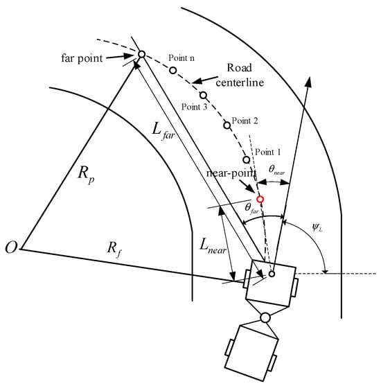
Figure 9.
Geometric relationship between near and far preview points.
The preview distance is a key parameter that significantly impacts the performance of the single-point preview algorithm. For the purpose of this study, was selected as a fixed value of 4 m after iterative tuning and validation in simulated underground mining scenarios.
The two-point preview algorithm expands the prediction range of the road ahead by introducing a second preview point. Typically, the first preview point is used for short-term path adjustments, while the second point predicts and corrects the vehicle’s long-term driving trajectory. By integrating the information from both preview points, the controller achieves precise short-term tracking while ensuring overall stability and anticipatory performance. The formula is as follows:
In this study, the near preview distance was selected as a fixed value of 1.5 m, while the far preview distance was set to 6 m. These values were chosen after iterative tuning and validation in simulated underground mining scenarios.
The multi-point preview algorithm builds upon single-point and two-point preview methods by selecting multiple preview points, significantly enhancing the perception and prediction capabilities for vehicle path tracking. The algorithm identifies multiple preview points positioned at different distances ahead of the vehicle. Near points are used for short-term path adjustments, while distant points provide long-term trajectory predictions. Each preview point’s deviation angle relative to the vehicle is calculated, and a weighted sum of these angles, based on distance-dependent weights, yields the total deviation angle.
Compared to single-point and two-point preview algorithms, the multi-point preview algorithm integrates short-term and long-term path information, offering comprehensive feedback to better handle complex environments such as continuous curves or obstacle-rich areas.
5. Results and Discussion
This section analyzes the experimental results and evaluates the performance of the boundary-aware multi-point preview control algorithm for autonomous driving in underground tunnels. The evaluation emphasizes safety and steering smoothness to comprehensively demonstrate the algorithm’s advantages. By comparing the proposed algorithm with single-point preview, two-point preview, and multi-point preview algorithms, the analysis highlights how the proposed approach achieves enhanced safety and smoother control in underground and highly constrained spaces.
5.1. Safety
Figure 10a,b illustrate the tracking trajectory and the corresponding variation in path deviation under Transport Route 1. In comparison, Figure 11a,b present the same performance metrics for Transport Route 2, and Figure 12a,b show the results for Transport Route 3. The statistical analyses for all three transport routes are summarized in Table 3, Table 4 and Table 5, which report key performance indicators, including mean tracking error, standard deviation, and maximum deviation. These metrics provide a quantitative basis for assessing the control accuracy, stability, and safety of the algorithm across different transport routes and road conditions.
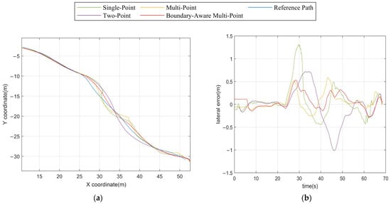
Figure 10.
Path tracking of different algorithms. (a) Path under Transport Route 1; (b) Lateral errors under Transport Route 1.
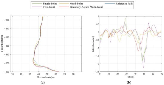
Figure 11.
Path tracking of different algorithms. (a) Path under Transport Route 2; (b) Lateral errors under Transport Route 2.
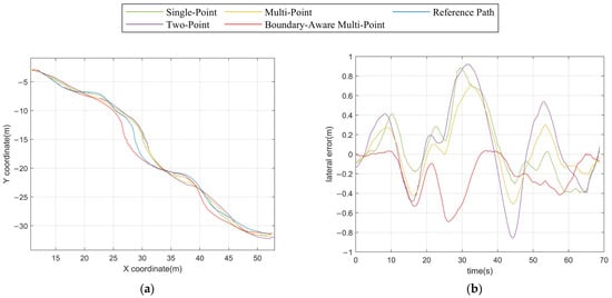
Figure 12.
Path tracking of different algorithms. (a) Path under Transport Route 3; (b) Lateral errors under Transport Route 3.
Table 3.
Statistical analysis of tracking performance under Transport Route 1.
Table 4.
Statistical analysis of tracking performance under Transport Route 2.
Table 5.
Statistical analysis of tracking performance under Transport Route 3.
In the results analysis, the lateral offset is calculated with respect to the LiDAR installation point, which is located at the center of the front axle. This reference point corresponds to the foremost interaction location between the vehicle and the tunnel environment and is directly associated with the acquisition of wall-based preview information. Since the proposed control framework does not rely on a predefined reference path, the lateral offset is introduced solely for performance evaluation and result interpretation. Using the front axle center as the reference point provides a clear geometric interpretation of the vehicle’s lateral position relative to the tunnel walls, avoids unnecessary coupling with the articulation angle, and ensures consistency between environmental perception and motion evaluation.
From Table 3, the boundary-aware multi-point preview control algorithm demonstrates superior performance in maintaining centerline tracking in highly confined spaces, achieving the smallest average error of 0.1564 m, standard deviation of 0.2102, and maximum error of 0.5284 m among all evaluated methods, highlighting its capability to outperform single-point, two-point, and multi-point algorithms in stability. From a tracking perspective, the boundary-aware multi-point preview method operates without relying on a reference path, instead dynamically determining the safe direction in real time. This feature enables the vehicle to naturally align with the tunnel centerline, as the determined direction inherently corresponds to the optimal road path, ensuring safe and efficient navigation in narrow environments while effectively reducing collision risks.
From Table 4, the boundary-aware multi-point preview achieves an average error of 0.2492 m, a standard deviation of 0.2796, and a maximum error of 0.6753 m, all of which are substantially lower than those of the single-point, two-point preview algorithms and multi-point. In contrast, the single-point preview algorithm demonstrates an average error of 0.2866 m, a standard deviation of 0.5812, and a maximum error as high as 1.758 m, highlighting its vulnerability to sudden terrain changes and obstacles that cause significant deviations from the centerline. Although the two-point preview algorithm slightly outperforms the single-point strategy in terms of standard deviation, its average error of 0.3822 m and maximum error of 2.1210 m reveal its instability in highly confined environments. The multi-point preview algorithm demonstrates an average error of 0.2682 m, a standard deviation of 0.3988, and a maximum error as high as 1.2050 m. These findings underscore that in the complex transport route, the boundary-aware multi-point preview strategy effectively adapts to trajectory variations and challenging terrains, ensuring superior stability and driving performance.
Table 5 presents the statistical comparison of tracking performance under Transport Route 3. The boundary-aware multi-point preview control algorithm achieves the best overall performance, with the lowest mean lateral error (0.2554 m), standard deviation (0.2497 m), and maximum error (0.6710 m) among all evaluated methods. These results indicate improved tracking accuracy as well as reduced lateral error fluctuations, which are essential for safe and stable operation in highly constrained underground environments. The single-point preview algorithm yields a mean error of 0.2614 m and a standard deviation of 0.3349 m, with a maximum error of 0.7079 m. Although its average error is close to that of the boundary-aware method, the larger standard deviation suggests inferior tracking consistency along the route. The two-point preview algorithm performs the worst, exhibiting the highest mean error (0.3534 m) and standard deviation (0.4255 m), together with a relatively large maximum error (0.7353 m). This indicates that increasing the number of preview points alone does not guarantee improved performance in complex environments.
It is worth noting that around t ≈ 29 s, the boundary-aware multi-point preview algorithm exhibits a lateral error trend opposite to that of the other three algorithms. One possible reason is related to the geometric discrepancy between the tunnel boundary and the nominal centerline. Specifically, when the local curvature of the tunnel wall deviates from that of the centerline, the boundary-based perception may induce a locally biased driving direction. As a result, the implicitly inferred traveling path derived from boundary geometry may shift in the opposite direction relative to the actual centerline, leading to a transient sign reversal of the lateral error. This phenomenon does not indicate instability of the proposed method; rather, it reflects its stronger responsiveness to local boundary features. In highly constrained underground environments, such behavior can be advantageous, as prioritizing boundary clearance over strict centerline adherence enhances collision avoidance capability and operational safety.
The conventional multi-point preview algorithm achieves moderate performance, with a mean error of 0.2915 m, a standard deviation of 0.3656 m, and a maximum error of 0.6981 m, but remains inferior to the boundary-aware multi-point strategy. Overall, the results confirm the effectiveness of incorporating boundary-awareness into multi-point preview control for complex transport routes.
Figure 13 illustrates the variations in the bidirectional proximity while driving on Transport Route 1; Table 6 summarizes the related statistical metrics, including mean value, standard deviation, maximum value, and minimum value. Similarly, Figure 14 and Table 7 present the corresponding analysis under Transport Route 2, and Figure 15 and Table 8 show the results for Transport Route 3. The statistical analyses for all three transport routes provide key indicators for evaluating the algorithm’s safety and responsiveness under different driving conditions.
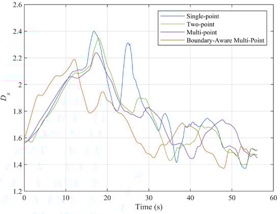
Figure 13.
The bidirectional proximity while driving on Transport Route 1.
Table 6.
Statistical analysis of under Transport Route 1.
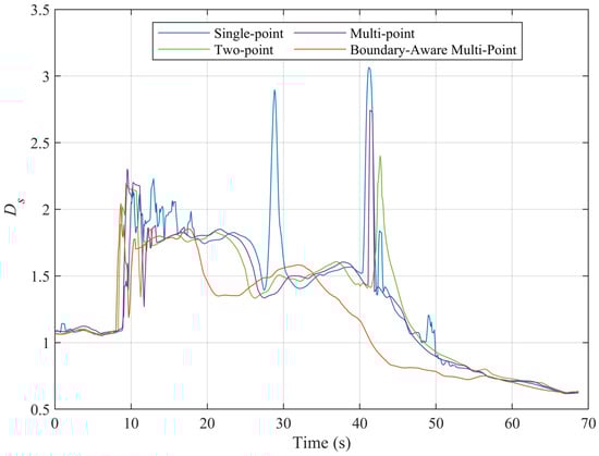
Figure 14.
The bidirectional proximity while driving on Transport Route 2.
Table 7.
Statistical analysis of under Transport Route 2.
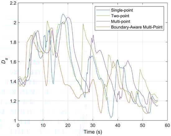
Figure 15.
The bidirectional proximity while driving on Transport Route 3.
Table 8.
Statistical analysis of under Transport Route 3.
By observing under identical road conditions for different control algorithms, we analyze the safety of vehicle operation. As shown in Table 6, the boundary-aware multi-point algorithm demonstrates the best overall performance across statistical analysis, emphasizing its advantage in maintaining a safe and stable distance from tunnel walls.
The boundary-aware multi-point algorithm achieves the smallest mean value 1.7091, indicating that it maintains a safer distance while navigating within the tunnel. This represents a 1.9% improvement compared to the multi-point algorithm, a 2.8% improvement compared to the two-point algorithm, and a notable 5.3% improvement compared to the single-point algorithm. With a standard deviation of 0.2174, the boundary-aware multi-point algorithm achieves the most consistent performance across all conditions, avoiding large variations and ensuring smoother operation. The boundary-aware multi-point algorithm records the smallest maximum value 2.1842, showing its ability to prevent excessive deviations from the safe location.
Additionally, the single-point preview shows a sudden change at 25 s, likely caused by its fixed preview distance, which prevents it from obtaining advanced information about distant obstacles, leading to abrupt adjustments. Overall, the boundary-aware multi-point preview demonstrates superior performance in dynamic environments, offering higher stability.
In Transport Route 2, the boundary-aware multi-point preview control strategy continues to exhibit significant advantages in terms of stability and safety relative to the distances from both the left and right walls. The data in Table 7 shows that the boundary-aware multi-point algorithm achieves the smallest mean value of 1.1572, with a standard deviation of 0.3961, a maximum of 2.0425, and a minimum of 0.6209. These results indicate that the boundary-aware multi-point algorithm demonstrates the best overall performance across statistical metrics, highlighting its ability to maintain a safe and stable distance from tunnel walls in more complex environments. In contrast, the single-point preview algorithm, despite having a mean value of 1.3355, shows a standard deviation of 0.5105, a maximum of 3.0653, and a minimum of only 0.6164. This suggests that the vehicle may, at times, come too close to the wall, posing a potential collision risk, especially in scenarios with sharp turns or sudden changes in curvature where control may be lost. The multi-point preview demonstrates more balanced performance but has a concerning maximum value of just 2.7432. This highlights the risk of the vehicle getting excessively close to the wall under extreme conditions, increasing the likelihood of collisions.
The data in Table 8 shows that the boundary-aware multi-point method achieves the lowest mean value of (1.3971) among all compared algorithms. This indicates that, on average, the articulated vehicle operates closer to the tunnel centerline while maintaining balanced distances to both walls. In contrast, the single-point, two-point, and conventional multi-point methods exhibit higher mean values of 1.4828, 1.5645, and 1.5565, respectively, suggesting less optimal wall-distance coordination under complex road geometry. In terms of stability, the boundary-aware multi-point approach also demonstrates the smallest standard deviation (0.2227), indicating reduced fluctuations of over time. This observation is consistent with the smoother curve shown in Figure 15, where abrupt oscillations are significantly suppressed compared to the other methods. The reduced variability implies that the vehicle can better adapt to changes in tunnel boundaries and road curvature, resulting in more consistent lateral positioning.
Regarding extreme values, the boundary-aware multi-point method records a lower maximum (1.9455) than the other strategies, effectively limiting excessive deviation from the tunnel center. Although its minimum value (1.0689) is slightly higher than that of the single-point method (1.0316), this indicates a more conservative and controlled behavior, avoiding overly aggressive proximity to either wall.
Overall, the boundary-aware multi-point preview strategy, by dynamically acquiring information from multiple preview points, can more comprehensively perceive changes in the confined underground space environment, ensuring stable driving near the centerline of the roadway. Considering the spatial relationship with both the left and right walls, the boundary-aware multi-point preview demonstrates lower standard deviation and a more balanced range. This indicates its effectiveness in reducing collision risks and enhancing the safety and stability of the vehicle in dynamic and complex environments.
5.2. Steering Smoothness
Figure 16 illustrates the variation in the articulation angle during vehicle operation under Transport Route 1, with Table 9 summarizing its standard deviation. Likewise, Figure 17 and Table 10 present the corresponding results for Transport Route 2, and Figure 18 and Table 11 show the results for Transport Route 3. The statistical analyses for all three transport routes provide quantitative insights into the vehicle’s maneuverability and stability under different driving conditions.
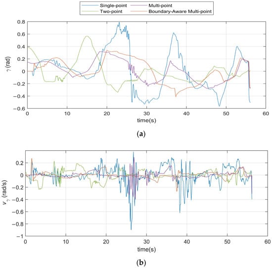
Figure 16.
Variation in articulation angle on Transport Route 1. (a) Articulation angle; (b) Articulation angle velocity.
Table 9.
Standard deviation of vehicle articulation angles on Transport Route 1.

Figure 17.
Variation in articulation angle on Transport Route 2. (a) Articulation angle; (b) Articulation angle velocity.
Table 10.
Standard deviation of vehicle articulation angles on Transport Route 2.
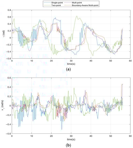
Figure 18.
Variation in articulation angle on Transport Route 3. (a) Articulation angle; (b) Articulation angle velocity.
Table 11.
Standard deviation of vehicle articulation angles on Transport Route 3.
As shown in Table 9, the boundary-aware multi-point algorithm demonstrates significant stability in steering angle variations, as evidenced by its noticeably smaller fluctuation amplitudes compared to other algorithms. A further analysis of the steering angle change rate reveals a standard deviation of 0.1274, which is 11.7% lower than the multi-point algorithm, 14.0% lower than the two-point algorithm, and a notable 49.1% reduction compared to the single-point algorithm. This significant reduction in standard deviation underscores the superior advantage of the boundary-aware multi-point algorithm. Its minimal steering angle change rate indicates smoother and more gradual directional adjustments, effectively avoiding abrupt directional shifts. This translates to enhanced vehicle stability and safety, particularly in complex and dynamic environments where sudden changes in steering can lead to instability or increased collision risks.
As shown in Table 10, the boundary-aware multi-point preview algorithm continues to demonstrate significant advantages in the stability of steering angle changes. A detailed analysis of the steering angle change rate reveals a standard deviation of 0.1892, which is 3.2% lower than the multi-point algorithm, 7.1% lower than the two-point algorithm, and a remarkable 36.4% reduction compared to the single-point algorithm. This performance indicates that the boundary-aware multi-point preview algorithm can effectively suppress sudden fluctuations during vehicle directional adjustments, ensuring smoother and more gradual steering. Consequently, it further enhances the driving comfort and control precision of the vehicle in dynamic environments.
From the articulation angle trajectories shown in Figure 18a, the single-point and two-point methods exhibit relatively larger oscillation amplitudes, particularly during sharp curvature transitions and boundary-constrained segments. In contrast, the multi-point and boundary-aware multi-point strategies demonstrate more restrained articulation angle variations, indicating improved coordination between the vehicle units when negotiating complex tunnel geometries. The angular velocity responses in Figure 18b further highlight the differences in motion smoothness. The single-point and multi-point methods present frequent high-frequency fluctuations and larger instantaneous peaks in , reflecting abrupt steering corrections and less stable articulation behavior. The two-point method partially mitigates these effects by incorporating additional preview information; however, noticeable oscillations are still present under rapidly changing boundary conditions.
Quantitatively, the standard deviation of provides a direct measure of articulation smoothness. As summarized in Table 11, the boundary-aware multi-point approach achieves the lowest standard deviation (0.1785) among all methods, indicating the most stable articulation behavior over the entire driving process. This value represents a reduction of approximately 23.9% compared with the single-point method and 26.9% compared with the conventional multi-point method. The two-point strategy yields an intermediate performance with a standard deviation of 0.1881, confirming the benefit of multi-preview information while still lacking explicit boundary awareness.
Such smooth adjustments not only enhance the vehicle’s stability in complex environments but also effectively mitigate the common yaw oscillation phenomenon encountered when driving in constrained underground spaces. Factors such as sharp turns, slopes, and uneven surfaces in these environments typically exacerbate vehicle oscillations, with frequent steering maneuvers causing significant body vibrations that affect driving comfort and safety. Additionally, reduced steering fluctuations contribute significantly to the structural safety of the vehicle. Frequent and intense steering not only adversely affects driving performance but also accelerates the wear and tear of vehicle components, increasing maintenance costs.
5.3. Control Parameters Analysis
Figure 19 illustrates the control parameters representing the weight values of different LiDAR rays at various angles during steering control. Specifically, a subset of angles, including 45°, 60°, 75°, 90°, 105°, 120°, and 135°, was selected for analysis. Figure 20, on the other hand, presents the verification of control parameters in speed control, demonstrating that their summation remains relatively stable or fluctuates within a specific range, confirming the consistency and reliability of the algorithm’s control strategy.
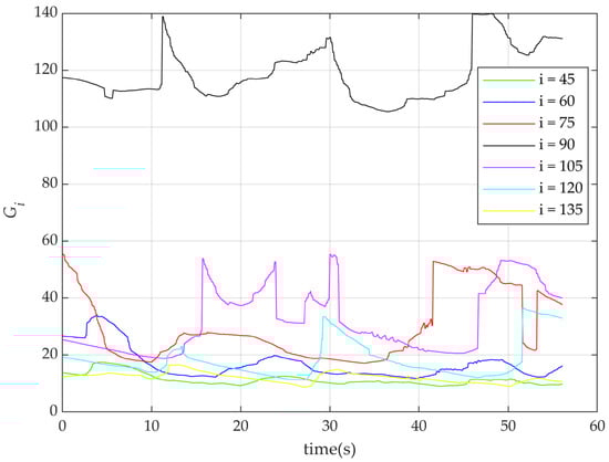
Figure 19.
Variation in the control parameter .
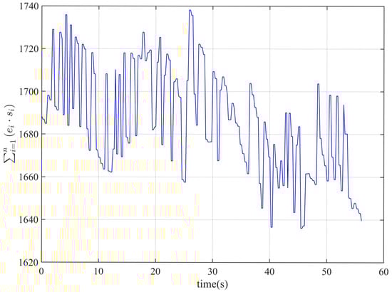
Figure 20.
Variation in control parameters in speed control.
The fluctuations of the curves in Figure 19 reflect the sensitivity of the nonlinear controller to varying angles and distance information. corresponds to the farthest preview angle, which is directly ahead of the vehicle. From Figure 19, it is evident that far points (e.g., ) carry higher weight and a larger gain value, indicating that the controller prioritizes distant information. This improves the system’s sensitivity to dynamic environmental changes, allowing for early adjustments in steering or speed, thereby optimizing the vehicle’s path-following performance. For closer points (e.g., , , , and ), the controller maintains more stable gain values, showing a focus on balancing the vehicle’s current driving state. The pronounced fluctuations at and demonstrate the controller’s ability to swiftly respond to distant environmental information when driving through complex terrain. This characteristic is particularly beneficial for ensuring the vehicle stays precisely near the centerline in narrow tunnels, enhancing both accuracy and safety.
The data in Figure 20 shows that the sum of products of and fluctuates within the range of 1660 to 1700, maintaining a relatively stable trend without significant deviations. This indicates that during the driving process, the LiDAR sensing range remains constant, with no substantial changes. The system is able to consistently detect targets and effectively monitor the surrounding environment. The stability of LiDAR sensing provides reliable data support for subsequent control decisions, particularly validating the correctness of the speed decision model. This further ensures the vehicle’s smooth and safe operation under varying road conditions.
5.4. Real-Time Performance
The data in Table 12 shows that the average processing time for the boundary-aware multi-point preview algorithm is 0.0610 s, representing a 58% increase compared to the single-point algorithm, a 19% increase compared to the two-point algorithm, and a 13% increase compared to the multi-point algorithm. This indicates that as the number of preview points increases, the computational complexity of the algorithm significantly rises, leading to longer response times. Nonetheless, the processing time remains shorter than the control cycle, meeting real-time requirements and ensuring that the system can promptly adjust in dynamic environments to maintain driving stability and safety.
Table 12.
Average runtime of path tracking algorithms.
This highlights that the single-point preview algorithm has a clear advantage in terms of real-time performance, enabling faster control adjustments, making it suitable for applications with high real-time requirements. The two-point preview algorithm provides a moderate predictive range while sacrificing some real-time performance, though it remains sufficient for most practical applications. Despite its higher computational demand and resulting delay due to processing multiple preview points, the boundary-aware multi-point preview algorithm excels in stability and adaptability, enabling it to meet the basic requirements in complex environments.
6. Conclusions
This paper proposes a boundary-aware multi-point preview control algorithm to address the challenges of autonomous driving for articulated underground mining vehicles in complex, highly confined underground environments. The algorithm enables articulated vehicles to directly determine driving direction by calculating control inputs in real time based on their driving state and LiDAR data, eliminating reliance on traditional path-planning methods. A simulation environment was constructed in ROS Noetic/GAZEBO 11 to validate the model’s performance, comparing it with single-point, two-point, and standard multi-point preview algorithms.
The experimental results demonstrate the effectiveness of the proposed control model in navigating complex underground mine tunnels, as well as its superior performance in steering stability, response speed, and overall system stability. Specifically, the boundary-aware multi-point preview model exhibited noticeable improvements in reducing steering angle fluctuations compared to both the single-point and two-point algorithms, while also outperforming the standard multi-point preview model. This highlights its ability to deliver smoother steering and enhanced stability, further improving overall system performance in challenging environments.
As the number of preview points grows, computational complexity increases exponentially. Future research will focus on optimizing the boundary-aware multi-point preview algorithm and exploring more efficient computational methods. As mining operations expand and evolve, resulting in more complex tunnel shapes and structures, the boundary-aware multi-point preview algorithm can be integrated with real-time updated mine maps or sensor data. This integration will enable adaptive responses to changing terrain conditions and allow dynamic adjustments to vehicle navigation strategies.
Although the performance of the proposed algorithm is validated through simulation-based experiments, the control strategy is fundamentally driven by geometric constraints and real-time LiDAR-based perception rather than relying on precise vehicle dynamic modeling. This design characteristic enhances its potential applicability to real underground mining scenarios, where vehicle parameters and operating conditions may vary. Nevertheless, further validation in real mine tunnel environments, as well as the consideration of additional dynamic effects and unexpected disturbances, will be important directions for future work.
Author Contributions
Conceptualization, Y.K.; methodology, S.H.; software, S.H.; validation, Y.K.; investigation, S.H.; resources, X.L.; data curation, S.H.; writing—original draft preparation, S.H.; writing—review and editing, Y.K.; visualization, S.H.; supervision, J.Y.; project administration, M.Z.; funding acquisition, J.Y. All authors have read and agreed to the published version of the manuscript.
Funding
This research was funded by the National Key Research and Development Plan program (Grant No. 2023YFC2907405), Key Research and Development Program Project of Shanxi Province (Grant No. 202402100101006), and Major Science and Technology Project of Shanxi Province (Grant number 202301150401011).
Data Availability Statement
The original contributions presented in this study are included in the article. Further inquiries can be directed to the corresponding author.
Conflicts of Interest
Author Xiao Lv was employed by Beijing BGRIMM Intelligent Technology. Author Ming Zhu was employed by Beijing BGRIMM Intelligent Technology. The remaining authors declare that the research was conducted in the absence of any commercial or financial relationships that could be construed as a potential conflict of interest.
Abbreviations
The following abbreviations are used in this manuscript:
| URDF | Unified Robot Description Format |
| ROS | Robot Operating System |
| MPC | Model Predictive Control |
| NMPC | Nonlinear Model Predictive Control |
| LQR | Linear Quadratic Regulator |
| LiDAR | Light Detection and Ranging |
References
- Li, J.-G.; Zhan, K. Intelligent Mining Technology for an Underground Metal Mine Based on Unmanned Equipment. Engineering 2018, 4, 381–391. [Google Scholar] [CrossRef]
- Cardenas, D.; Loncomilla, P.; Inostroza, F.; Parra-Tsunekawa, I.; Ruiz-del-Solar, J. Autonomous Detection and Loading of Ore Piles with Load–Haul–Dump Machines in Room and Pillar Mines. J. Field Robot. 2023, 40, 1424–1443. [Google Scholar] [CrossRef]
- Tampier, C.; Mascaró, M.; Ruiz-del-Solar, J. Autonomous Loading System for Load–Haul–Dump (LHD) Machines Used in Underground Mining. Appl. Sci. 2021, 11, 8718. [Google Scholar] [CrossRef]
- Xiao, W.; Liu, M.; Chen, X. Research Status and Development Trend of Underground Intelligent Load–Haul–Dump Vehicles: A Comprehensive Review. Appl. Sci. 2022, 12, 9290. [Google Scholar] [CrossRef]
- Fue, K.; Porter, W.; Barnes, E.; Li, C.; Rains, G. Autonomous Navigation of a Center-Articulated and Hydrostatic Transmission Rover Using a Modified Pure Pursuit Algorithm in a Cotton Field. Sensors 2020, 20, 4412. [Google Scholar] [CrossRef] [PubMed]
- Dekker, L.G.; Marshall, J.A.; Larsson, J. Experiments in Feedback Linearized Iterative Learning-Based Path Following for Center-Articulated Industrial Vehicles. J. Field Robot. 2019, 36, 955–972. [Google Scholar] [CrossRef]
- Nayl, T.; Nikolakopoulos, G.; Gustafsson, T.; Kominiak, D.; Nyberg, R. Design and Experimental Evaluation of a Novel Sliding Mode Controller for an Articulated Vehicle. Robot. Auton. Syst. 2018, 103, 213–221. [Google Scholar] [CrossRef]
- Yang, F.; Cao, X.; Xu, T.; Ji, X. A Skid-Steering Method for Path-Following Control of Distributed-Drive Articulated Heavy Vehicles. IEEE Access 2022, 10, 31538–31547. [Google Scholar] [CrossRef]
- Tian, J.; Shen, Y.; Zhong, Q. Path Tracking of Distributed Drive Articulated Vehicle Coordinated with Differential Torque. In Proceedings of the 2021 Chinese Automation Conference, Shanghai, China, 26–28 July 2021; pp. 453–458. (In Chinese) [Google Scholar]
- Yu, H.; Zhao, C.; Li, S.; Wang, Z.; Zhang, Y. Pre-Work for the Birth of Driverless Scraper (LHD) in the Underground Mine: The Path Tracking Control Based on an LQR Controller and Algorithm Comparison. Sensors 2021, 21, 7839. [Google Scholar] [CrossRef]
- Zhou, B.; Su, X.; Yu, H.; Guo, W.; Zhang, Q. Research on Path Tracking of Articulated Steering Tractor Based on Modified Model Predictive Control. Agriculture 2023, 13, 871. [Google Scholar] [CrossRef]
- Shi, J.; Sun, D.; Qin, D.; Hu, M.; Kan, Y.; Ma, K.; Chen, R. Planning the Trajectory of an Autonomous Wheel Loader and Tracking Its Trajectory via Adaptive Model Predictive Control. Robot. Auton. Syst. 2020, 131, 103570. [Google Scholar] [CrossRef]
- Bai, G.; Liu, L.; Meng, Y.; Luo, W.; Gu, Q.; Ma, B. Path Tracking of Mining Vehicles Based on Nonlinear Model Predictive Control. Appl. Sci. 2019, 9, 1372. [Google Scholar] [CrossRef]
- Guan, S.; Wang, J.; Wang, X.; Shi, M.; Lin, W.; Chen, W. Dynamic Hyperparameter Tuning-Based Path Tracking Control for Robotic Rollers Working on Earth-Rock Dams under Complex Construction Conditions. Autom. Constr. 2022, 143, 104576. [Google Scholar] [CrossRef]
- Tan, S.; Zhao, X.; Yang, J.; Zhang, W. A Path Tracking Algorithm for Articulated Vehicle: Development and Simulations. In Proceedings of the 2017 IEEE Transportation Electrification Conference and Expo, Asia-Pacific (ITEC Asia-Pacific), Harbin, China, 7–10 August 2017; pp. 1–6. [Google Scholar]
- Dou, F.; Meng, Y.; Liu, L.; Gu, Q. A Novel Relative Navigation Control Strategy Based on Relation Space Method for Autonomous Underground Articulated Vehicles. J. Control Sci. Eng. 2016, 2016, 2352805. [Google Scholar] [CrossRef]
- Wiberg, V.; Wallin, E.; Nordfjell, T.; Servin, M. Control of Rough Terrain Vehicles Using Deep Reinforcement Learning. IEEE Robot. Autom. Lett. 2022, 7, 390–397. [Google Scholar] [CrossRef]
- Zhao, S.; Wang, L.; Zhao, Z.; Bi, L. Study on the Autonomous Walking of an Underground Definite-Route LHD Machine Based on Reinforcement Learning. Appl. Sci. 2022, 12, 5052. [Google Scholar] [CrossRef]
- Andersen, H.; Chong, Z.J.; Eng, Y.H.; Pendleton, S.; Ang, M.H. Geometric Path Tracking Algorithm for Autonomous Driving in Pedestrian Environment. In Proceedings of the 2016 IEEE International Conference on Advanced Intelligent Mechatronics (AIM), Banff, AB, Canada, 12–15 July 2016; pp. 1669–1674. [Google Scholar]
- Li, S.; Xu, B.; Hu, M. Multi-Point Preview Path Tracking Method for Articulated Vehicles Based on Dynamic Model Predictive Control. Automot. Eng. 2021, 43, 1187–1194. [Google Scholar]
- Koenig, N.; Howard, A. Design and use paradigms for Gazebo, an open-source multi-robot simulator. In Proceedings of the IEEE/RSJ International Conference on Intelligent Robots and Systems (IROS), Sendai, Japan, 28 September–2 October 2004; pp. 2149–2154. [Google Scholar]
Disclaimer/Publisher’s Note: The statements, opinions and data contained in all publications are solely those of the individual author(s) and contributor(s) and not of MDPI and/or the editor(s). MDPI and/or the editor(s) disclaim responsibility for any injury to people or property resulting from any ideas, methods, instructions or products referred to in the content. |
© 2026 by the authors. Licensee MDPI, Basel, Switzerland. This article is an open access article distributed under the terms and conditions of the Creative Commons Attribution (CC BY) license.